Article

Research on Wind Turbine Blade Surface Damage Identification Based on Improved Convolution Neural Network

1
Software Technology Institute, Dalian Jiaotong University, Huanghe Road, Dalian 116028, China
2
Liaoning Key Laboratory of Welding and Reliability of Rail Transportation Equipment, Dalian Jiaotong University, Huanghe Road, Dalian 116028, China
3
Dalian Key Laboratory of Welded Structures and Its Intelligent Manufacturing Technology (IMT) of Rail Transportation Equipment, Huanghe Road, Dalian 116028, China
*
Author to whom correspondence should be addressed.
Appl. Sci. 2022, 12(18), 9338; https://doi.org/10.3390/app12189338
Submission received: 24 August 2022 / Revised: 13 September 2022 / Accepted: 14 September 2022 / Published: 18 September 2022

Abstract

:
Wind turbine blades are easily affected by the working environment and often show damage features such as cracks and surface shedding. An improved convolution neural network, ED Net, is proposed to identify their damage features. An EAC block based on the improved asymmetric convolution is introduced which strengthens the feature extraction during convolution. A DPCI_SC block, which is improved based on the attention module, is embedded to enhance the ability to obtain spatial location information of the damage. GELU is used as the activation function. The loss function is smoothed and labeled during training. Finally, three sets of experiments were conducted. Experiment 1 confirmed the efficacy of the ED Net for identifying damaged wind turbine blades. Experiment 2 confirmed the efficacy of the relevant improvements proposed in this work. Experiment 3 compares the recognition of wind turbine blade damage by commonly used lightweight networks and shows that the ED Net model proposed has a better performance with an accuracy range of 99.12% to 99.23% and a recall of 99.23%

1. Introduction

1.1. Motivation

Global energy consumption has increased in recent decades and is predicted to continue in the future. Historically, fossil fuels have fulfilled electricity demand, but worries about sustainability have spurred a change in attention to renewable energy sources [1,2]. Governments and international organizations have spent considerably on the development of energy-seeking and renewable energy sources in the past several decades.
Some of the most popular renewable energy generating systems are wind power, hydroelectric power, photovoltaic power, solar thermal power, and geothermal power. Among these, wind power generation is the most extensively utilized renewable energy technology in the world. The overall potential for wind turbines installed globally is 651 GW by the end of 2019, an increase of 59.667 GW in 2019 alone, which has an approximate growth of 19% in the global wind power market [3].
Wind turbine blades, being one of the most significant components of a wind turbine, have a direct impact on its power-generating efficiency. In the all-weather operation of wind turbines, the blades are more vulnerable to strong winds, sandstorms, lightning, rain, and snow, a statistical analysis of wind farm failures in Sweden between 1997 and 2005 showed that blade damage accounted for 13.4 percent of all failures, while the gearbox and generator accounted for 9.8 percent and 5.5 percent respectively [4], so it is necessary to focus on regular inspection of wind turbine blades. In the beginning, the most common method for inspection of a wind turbine blade was a manual examination, with the workers using a telescope to monitor the damage status of the blades. This type of inspection is time-consuming and laborious. The blade image in the telescope is frequently blurred when observed with the human eye, and the inspection effect is not satisfactory due to the influence of weather and light. On the other hand, the timelier the maintenance and care of blades, the better. When there is light wear, a timely repair can prevent the wear from deteriorating. However, if the problem is not addressed promptly, the wear on the blade may gradually degrade into fractures, resulting in blade fracture and fall off, causing major economic losses and possible safety accidents. Therefore, investigating a quick and accurate approach for detecting damage to the wind turbine blade has important practical engineering significance and application value.

1.2. Related Works

Numerous academics have focused on the damage identification of wind turbine blades. Some have utilized fiber optic sensing, thermography, shearography, acoustic sequences, and other techniques. For example, Md Abu Shohag et al. [5] used fiber optic sensing techniques. Wind turbine blades had in situ triboluminescent optical fiber sensors embedded in the adhesive layer. The in situ triboluminescent optical fiber sensors can detect damage near the blade adhesive joint in real-time, according to tests. Long-pulse thermography was proposed by Jensen Friederike [6] et al. for detecting coating peeling and material damage defects in wind turbine blades. Despite the non-vertical detection view, this technology can guarantee good detection results. The shearography was improved by Zhiyao Li [7] et al. A novel shearography system based on a simple setup of Michelson interferometry using pixelated spatial phase shift was used in the study for the dynamic inspection of delamination defects on a real wind turbine blade. The obtained results show that the proposed approach is capable of accurately detecting defects and dynamically deriving phase-changing sequences. Kai Aizawa [8] et al. conducted an acoustic array study by placing an audio speaker inside a wind blade to collect and observe the sound emitted by the blade to detect structural damage.
The methods for identifying wind turbine blade damage proposed from the above perspectives have good accuracy rates, but they often have limitations. Some methods are expensive and time-consuming, and some can only detect a single damage defect, making them unsuitable for use in the actual industrial environment.
Later, some academics proposed machine learning-based methods for damage detection of the wind turbine blade. For example, A. Joshuva et al. [9] used the decision tree approach in machine learning to obtain the desired features by recording the vibration signals of the leaves based on their various damage states using histogram features. Jaramillo Francisco et al. [10] proposed a wind turbine blade fatigue damage diagnosis method based on a Bayesian classifier, which extracted the input features required for the Bayesian framework from the vibration signal of the blade and then identified the wind turbine blade damage based on the output of the classifier. Chandrasekhar et al. [11] investigated a new machine-learning technique for damage detection of operating wind turbine blades. Using structural health monitoring techniques and Gaussian processes, damage to the blade was determined and identified. W. Long et al. [12] proposed a data-driven framework for the automatic detection of wind turbine blade surface cracks based on UAV images. Haar-like features are used to describe the crack regions and a cascade classifier is trained to detect the cracks. To sum up, methods based on machine learning are frequently straightforward and efficient, but they cannot automatically extract flawed characteristics and typically demand a great deal of preparation.
Recently, convolutional neural networks have been widely used in detection techniques due to their advantages of simple operation, automatic extraction of feature information, and high identification efficiency. L. Fan et al. [13] proposed an effective method for multi-feature fusion using a one-dimensional convolutional neural network model. It was used to improve the detection performance of low signal-to-noise ratio magnetic anomaly signals. L. Wang et al. [14] designed a portable vision sensor system using the simplified and optimized lightweight model MobileNet_SSD for detecting spray deposition in UAV applications. Y.-H. Nho et al. [15] proposed a novel generative adversarial network (GAN)-based fall detection method using a heart rate sensor and an accelerometer.
Thus, some academics have employed deep learning techniques to address this problem. A. Reddy et al. [16] proposed an approach using the deep learning method. Based on the convolution neural network, classification and recognition of various fault images such as lightning strikes, cracking, and corrosion were achieved. Juhi Patel et al. [17] used convolutional neural network VGG16-RCNN for wind turbine blade surface damage detection. Zhang J. et al. [18] evaluated the performance of the currently popular YOLOv3, YOLOv4, and Mask R-CNN deep learning algorithms for detecting and classifying defects by type of wind turbine blades and proposed an image-enhancement-based Mask R-CNN algorithm (IE Mask R-CNN). Deep learning was applied by Zhu Jiawei et al. [19] to the recognition of wavelet transform blade defects. For the rapid detection of wavelet transform blade defects, a residual network structure based on the fusion of multiple features was proposed. Based on YOLOv3, Dipu Sarkar et al. [20] proposed a wavelet transform blade damage recognition model for UAV images. The Super-Resolution CNN (SRCNN) method was used to identify low-resolution UAV images and convert them to high-resolution images. YOLOv3 was then applied to aerial images to detect damage to turbine blades. Zhang Zhiqiang et al. [21] proposed a novel algorithm by enhancing RNN to achieve rapid warning of icing faults in wind turbine blades. First, the algorithm selects the features that have a significant impact on wind turbine blade icing faults based on the mean impact value (MIV) index, and then the T-distributed Stochastic Neighbor Embedding (TSNE) algorithm reduces the dimensions of the selected features, which drastically decreases the processing time of the algorithm. Finally, the processed data are inputted into the RNN model for wind turbine blade icing prediction. Rezamand, M. et al. [22] proposed a new real-time hybrid fault detection strategy for wind turbine blades. The suggested fault detection system employed an integrated Generalized Regression Neural Network Ensemble for Single Imputation (GRNN-ESI), Recursive Principal Component Analysis (RPCA), and wavelet-based Probability Density Function (PDF) methods to detect incipient faults in an early stage.
As a result of extensive research conducted by academic researchers, the structure of convolution neural networks has been continuously improved, and the efficiency of the task used for damage detection of wind turbine blades has gradually increased. However, when a network performs a convolutional operation, the loss of feature information details of the image is unavoidable. Such damage characteristics of the blade as the length and depth of the crack and the size and shape of wear are variable. As a consequence, lost information detail frequently leads to errors in identification, so the identification accuracy has room for improvement.

1.3. Contributions and Outline

To solve this problem, a novel ED Net consisting of Enhanced Asymmetric Convolution blocks and Double Pooling Concatenated Input Squeeze-and-excitation Blocks is proposed. In this study, we show the following:
(1)
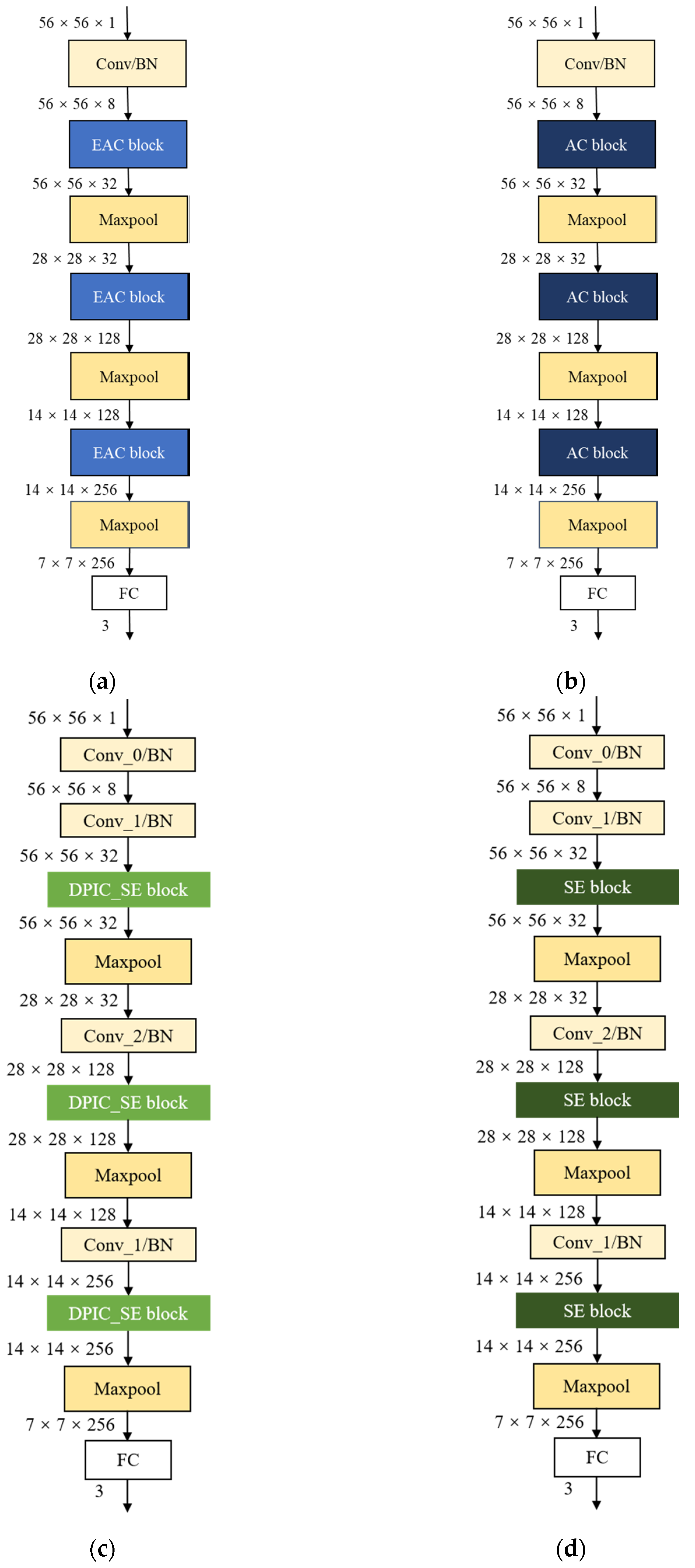
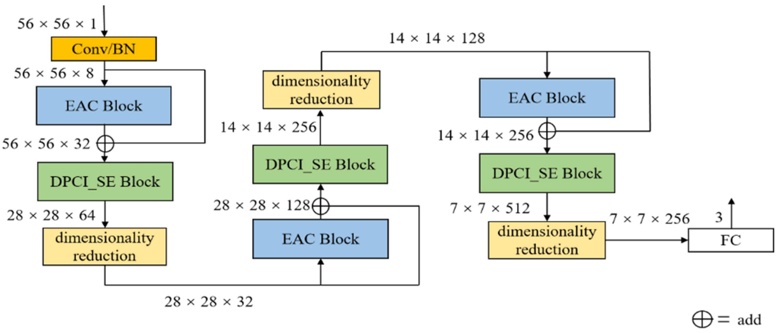
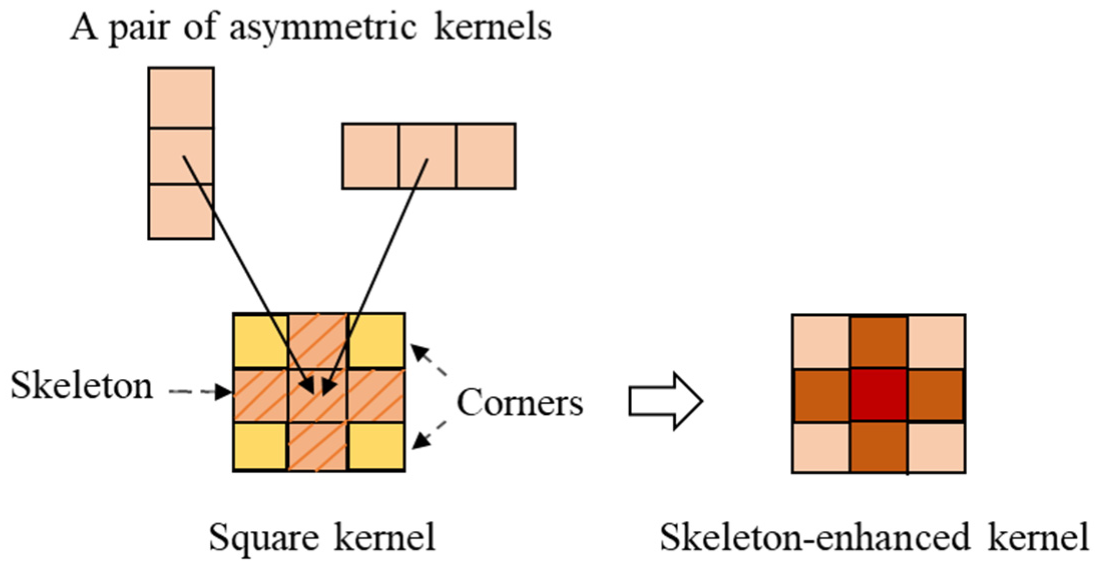
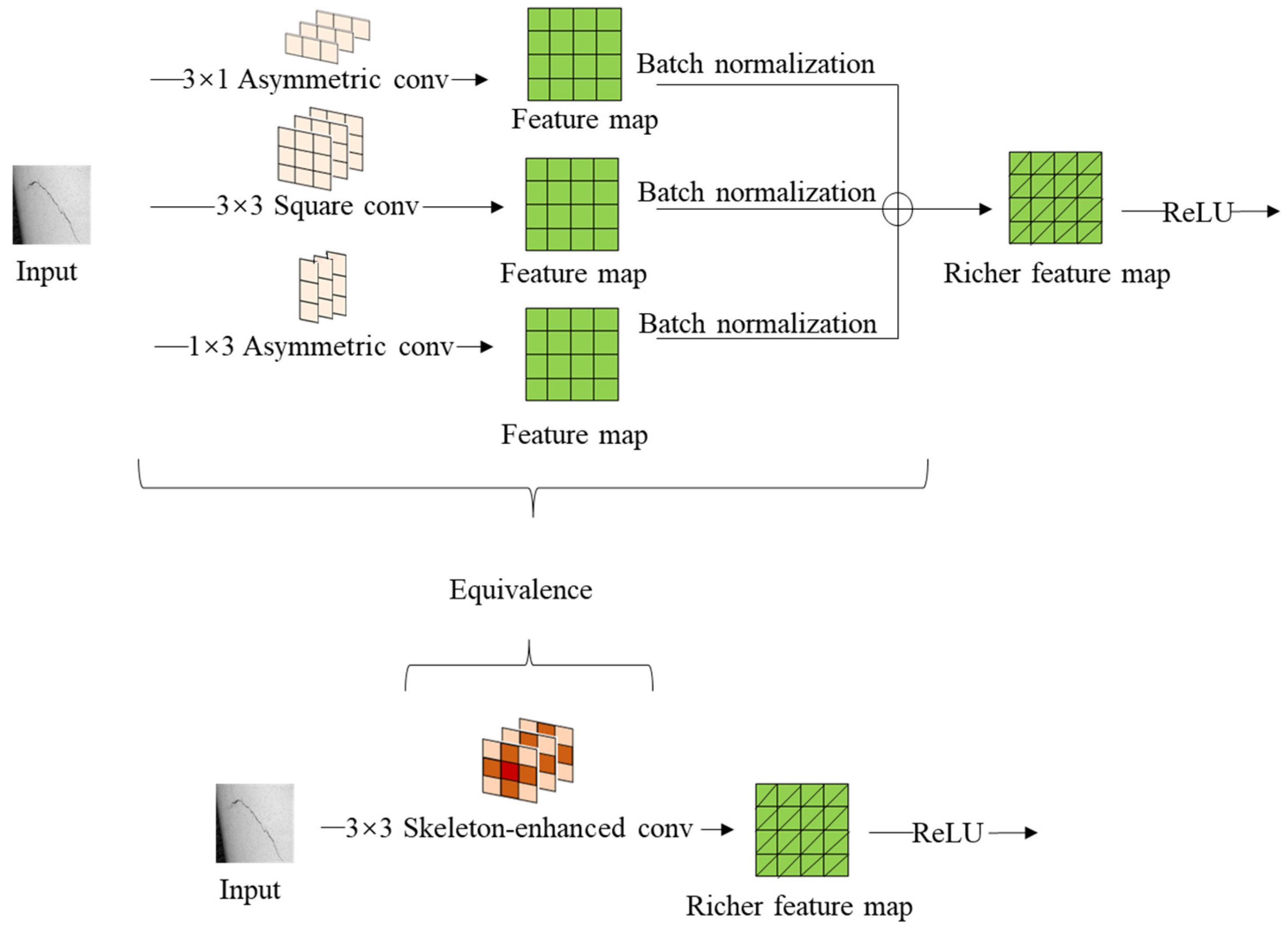
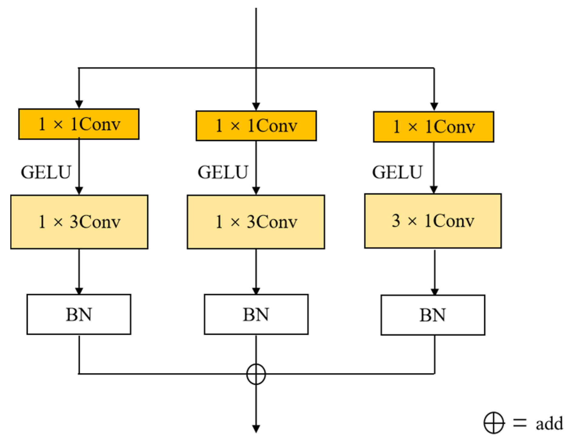
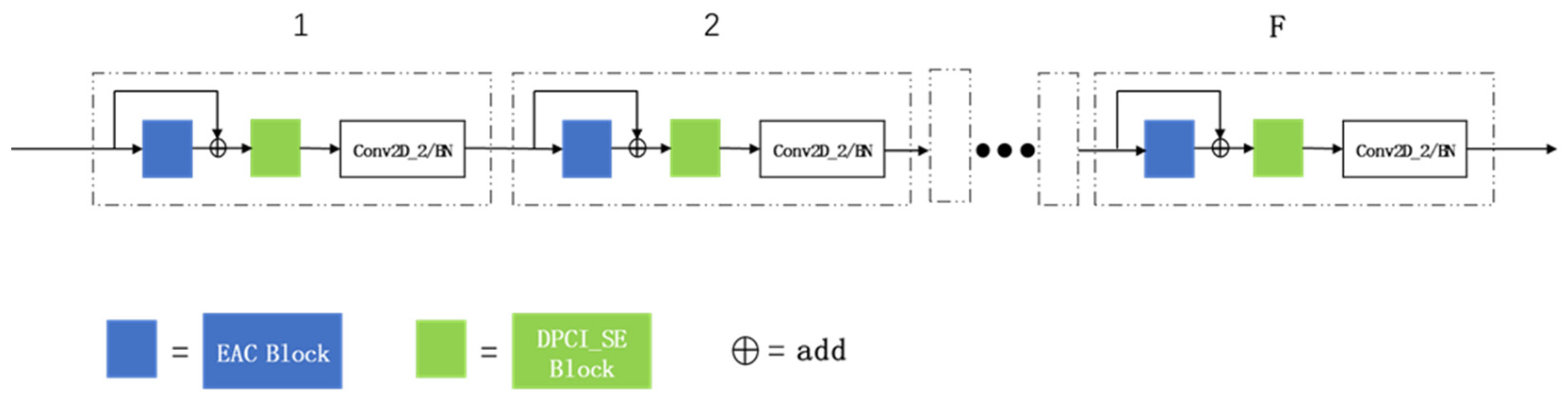
The Enhanced Asymmetric Convolution block (EAC block) is used in the suggested ED Net, which is an improvement on Enhanced Asymmetric Convolution to improve feature extraction.
(2)
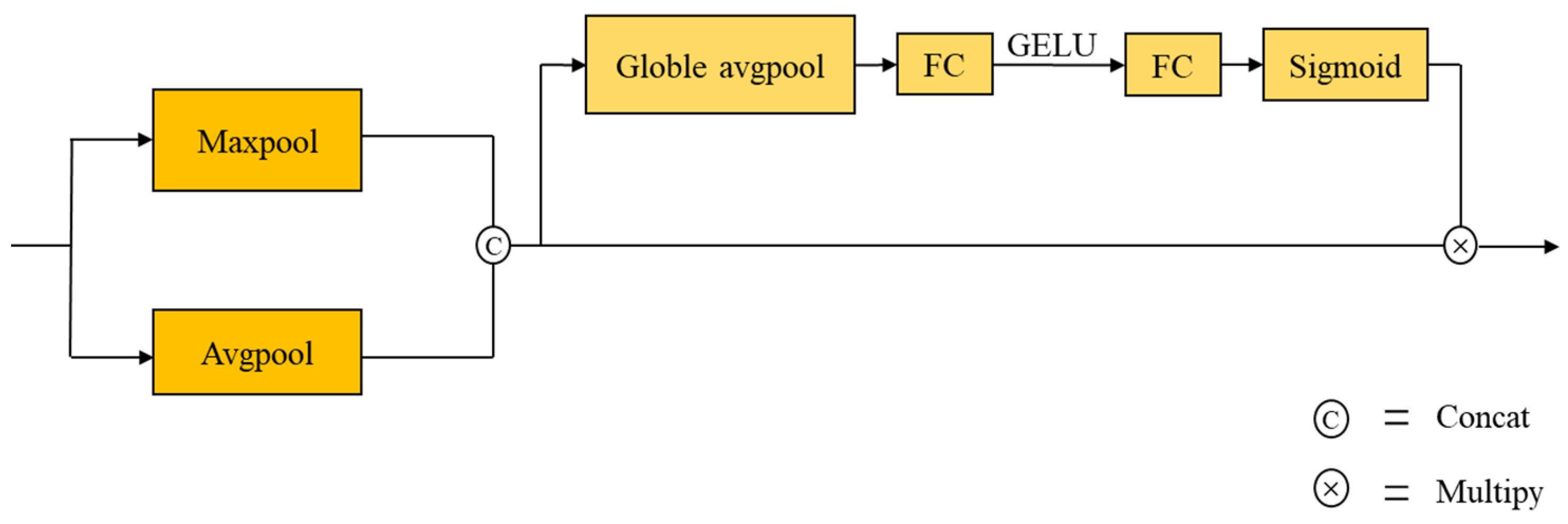
The Double Pooling Concatenated Input Squeeze-and-excitation Block (DPCI-SE Block) is used in the ED Net. Based on Squeeze-and-excitation Block (SE Block) [23], DPCI-SE Block is a better attention module. It is added to enhance the acquisition of spatial location information of damaged special folds.
(3)
The accuracy of ED Net for wind turbine blade surface damage identification mission is between 99.12% and 99.23% in this paper, and the recall is 99.43%. ED Net outperforms some common lightweight CNNs in terms of overall performance.
Section 2 contains some descriptions of the principles of the improved methods for convolutional neural networks used in this paper. In Section 3, three experiments on ED Net are mentioned and the experimental results are discussed. Experiment 1 determines the overall structure of ED Net and verifies its effectiveness for the wind turbine blade damage identification task. Experiment 2 verifies the effectiveness of the relevant improvements made in this paper. Experiment 3 compares the recognition of wind turbine blade damage by the currently used lightweight networks and measures that the ED Net model proposed in this paper has a good comprehensive performance. Section 4 provides concluding remarks and an outlook on subsequent work.

2. Materials and Methods

2.1. Overview of Convolutional Neural Network

A convolutional neural network (CNN) is a multilayer supervised feedforward neural network designed to learn abstract features of the input by alternately stacking convolutional kernels and pooling operations. CNNs are characterized by weight sharing and sparse connectivity and generally consist of a convolutional layer, a pooling layer, and a fully connected layer. The convolutional layer consists of multiple convolutional units that perform different operations by adjusting parameters through a backpropagation algorithm [24]. The convolutional layer is used to extract the feature map using a convolutional kernel. The convolution kernel can be considered as the matrix. For example, a convolution kernel is set up as a 3 × 3 matrix and the size of the image to be convolved is 5 × 5. The convolution kernel will perform a convolution operation on the first area of the image to be convolved, and the result of this convolution calculation will be used as a point on the output feature map, as shown in Figure 1. Then, the convolution kernel will slide over the input image and perform the next convolution operation to output the next point on the feature map. The above operations are repeated until the complete feature map is output.
The pooling layer can further filter the image’s object features, eliminate unimportant data information, reduce the number of parameters, identify important feature information, simplify the computation procedure, and accelerate the training speed. The fully connected layer is responsible for further analyzing the data extracted by the convolutional and pooling layers and sorting them by regression functions. The advantage of using CNN for feature extraction of images is that the user does not have to care at all about which specific features are present. This greatly solves the previous problem of certain features being difficult to recognize with the human eye. Therefore, CNNs are widely used in material defect, bridge damage, and plant disease identification missions.

2.2. The Basic Structure and Principle of ED Net

2.2.1. The Structure of ED Net

The overall architecture of the ED Net model proposed in this paper is depicted in Figure 2.
As shown in Figure 2, the first convolutional layer of ED Net is used to enhance the dimensionality of the feature map, followed by the introduction of a BN layer for data normalization to improve the convergence speed of the model. Then there is an AC Block with residual connections. It is based on the asymmetric convolution structure improvement, which enhances the extraction of feature information by the convolution operation by strengthening the content extracted at the convolution kernel skeleton. After which, there is a Double Pooling Concatenated Input SE Block (DPCI _SE Block), which is based on the SE block to obtain more global and local feature channel data. The final layer is the dimensionality reduction layer, which consists primarily of a convolutional layer with a convolutional kernel size of 1. The objective is to reduce the dimensionality of the feature map and the number of internal model parameters computed. A group of synthesized structures includes an EAC Block, a DPCI_SE Block, and a dimensionality reduction layer. After three groups of such synthesized structures, there are the fully connected layer and the SoftMax layer. The complete Flowchart of ED Net training is shown in Figure 3.

2.2.2. GELU Activation Function

In the modeling process of neural networks, an important property of the model is nonlinearity, and for the model’s generalization ability, it is necessary to include a stochastic regular. The input to the model is determined by both the stochastic regularity and the nonlinear activation. In the field of activation functions, these common activation functions have their drawbacks. Sigmoid is easily saturated. Exponential Linear Unit (ElU) and Rectified Linear Unit (ReLU) lack the stochastic factor. However, Gaussian Error Linear Unit (GELU) introduces the idea of stochastic regularity in activation, which is intuitively more natural. Literature [25] confirms that GELU is a high-performance neural network activation function that incorporates stochastic regularity in activation, a probabilistic description of neuron input. It is expressed as:
GELU ( x ) = x ϕ ( x )
x represents the activated input value of the current neuron, whereas ϕ ( x ) represents the cumulative distribution of the Gaussian normal distribution, or the definite integral of the Gaussian distribution in the interval (−∞, x]. This is more intuitively consistent with natural understanding and helps to increase the model’s nonlinear capability. The conventional ReLU activation function is designed to be replaced by GELU in the ED Net model proposed in this paper to improve recognition accuracy.

2.2.3. Smooth Labeling of the Loss Function

The loss function will have better resistance to overfitting after the smooth labeling improvement. The loss function is essentially designed to encourage the output of the model to approach the corresponding sample labels. In the network learning process of traditional one-hot encoded labels, the loss function encourages the model to predict the probability of being the target category to be close to 1, and the probability of being the non-target category to be close to 0. The traditional one-hot encoded label vector is y i and is expressed as:
y i = { 1 , i f ( i = y ) 0 , o t h e r w i s e
where y represents the target label and i represents the output value. However, this is likely to result in overfitting. If the output value is extremely close to the sample label, but this training sample is incorret, this can be extremely detrimental to the model. Because a faulty sample must be learned during the training process and has a very high probability of occurring, this will have a significant effect on the posterior probability estimation, and sometimes the classes are not unrelated to one another, leading to a degree of overfitting if the output probability interval is large. Consequently, the probability interval can be appropriately reduced. The impact of incorrect labeling can be mitigated by adjusting the distance between the extremes. The new label vector y i ^ replaces the conventional one-hot encoded label vector and is expressed as:
y i ^ = { 1 ε , i f ( i = y ) ε M , o t h e r w i s e
where ε represents a small positive real hyperparameter (typically assumed to be 0.1), while M represents the total number of multicategories. Therefore, the extremes are 1 − ε and ε / M , rather than 1 and 0.
Smoothing the labels is equivalent to adding noise to the true distribution to prevent the model from being overconfident about the correct labels, resulting in a relatively small difference between the output values of the predicted positive and negative samples. This method prevents overfitting to some extent, reduces the impact of incorrect labels, and enhances the model’s generalization ability.

2.2.4. EAC Block

The convolution operation on an image is essentially a matrix operation; consequently, the convolution operation possesses the characteristics of the matrix multiplication distribution law, in other words, multiple convolution sum operations can be synthesized into a single convolution operation, as shown in Equation (4):
P k ( 1 ) + P k ( 2 ) + P k ( 3 ) = P ( k ( 1 ) k ( 2 ) k ( 3 ) ) = P K
where P represents the input feature map. k ( 1 ) , k ( 2 ) , and k ( 3 ) represent three convolution kernels compatible with size. Equation (4) reflects the fact that the following three operations are equivalent: performing k ( 1 ) , k ( 2 ) , and k ( 3 ) convolution operations separately on the feature map P and then adding them, adding k ( 1 ) , k ( 2 ) , and k ( 3 ) before performing convolution operations with the feature map P, and using a convolution kernel K matching k ( 1 ) , k ( 2 ) , and k ( 3 ) to perform convolution operations on the feature map P.
In the literature [26], it was mentioned that the skeleton weights of a convolution kernel are usually large and removing these weights can lead to more accuracy degradation than removing the weights in the corners. In other words, the distribution of the learned feature information by the square convolutional kernels is uneven. Therefore, a pair of asymmetric kernels can be added to the corresponding positions of the matched square convolutional kernels for reinforcing the skeleton information as shown in Figure 4. Moreover, it can be concluded from Equation (4) that the square convolutional kernels with reinforced skeleton add no extra computational effort to the network model.
Asymmetric convolution block (AC Block) was proposed in the literature [26]. A convolution with inconsistent length and width dimensions of the convolution kernel, such as 3 × 1 or 1 × 3, is called an asymmetric convolution. The authors replace the single 3 × 3 square convolution with another convolution consisting of a pair of asymmetric convolutions and a square 3 × 3 convolution, forming a total of three convolution branches in parallel. Li X, Ma X. [27] proposed an image semantic segmentation method and improved the expression ability of the backbone network based on ACB. Hu L, Zhang H, Wang Z, et al. [28] proposed a novel self-supervised monocular depth system. Their depth system utilized ACB, which could improve the ability to extract features during training. The asymmetric convolution in the AC Block can improve the network’s robustness to image flipping when the network is in the training phase. When the network enters the deployment phase following the completion of training, the three parallel branches respectively perform feature extraction on the image. Then, the batch normalization is carried out and added together. The output is equivalent to a skeleton-enhanced convolution kernel extraction feature extraction result. This process is illustrated in Figure 5 and the literature [26] provides a detailed derivation of the equations for this.
In the convolution operation, the main feature information located at the location of the convolution kernel skeleton is emphasized. This design permits fusing the additional feature information extracted by the asymmetric convolutional layers during the training phase of the network without incurring any additional computational effort during the deployment phase. This improves the network’s performance when inference is implemented.
In this paper, the Enhanced Asymmetric Convolution Block (EAC Block) is constructed based on AC Block. The internal structure of the EAC Block is shown in Figure 6. The EAC Block adds a convolution layer with a convolution kernel size of 1 to each branch and then goes through the smooth-labeled GELU activation function, which further enhances the nonlinearity of the module and enhances its expressiveness.

2.2.5. DPCI_SE Block

Double Pooling Concatenated Input SE Block (DPCI_SE Block) is based on the SE block, the key characteristic of which is to split channels and acquire the learning weights of each channel depending on the loss. This strategy lets the effective feature take up more learning weight and the ineffective or poor feature take up less learning weight so that the model can receive better training results. The process is divided into the squeeze phase, the excitation phase, and the reweight phase. The basic idea of the squeeze phase is to compress the feature input down the spatial dimension, use a global average pooling to improve the perceptual field, and match the dimension of the output with the number of input feature channels. The global information z C obtained from each channel feature map is expressed as:
z C = F sq ( u c ) = 1 H × W i = 1 H j = 1 W u c ( i , j )
where u c represents the feature map of each channel, H represents the height of the feature map, and W represents the width of the feature map. The basic idea of the excitation phase is based on the correlation of feature channels, each feature channel gets a weight, and the weight is used to indicate the importance of the feature channel. The input is the global information obtained in the Excitation phase, after a layer of a fully connected layer, ReLU activation function, fully connected layer for the excitation operation, and the sigmoid function to limit the number out results in the [0, 1] interval. The output learning weight s is expressed as:
s = F e x ( z , W ) = σ s i g m o i d ( W 2 σ ReLU ( W 1 z ) )
W 1 and W 2 represent the weight matrix of the two fully connected layers. W 1 C r × C , W 2 C × C r , r is the decay factor, and the literature [21] states that this value is 16. Finally, reweight phase is to treat the weights obtained in the Excitation phase as the importance of this channel features, and weighs them to the previous features channel by channel. The important features are enhanced and the unimportant features are weakened. This operation can be expressed as:
x c ˜ = s c u c
where u c is the feature map of the original channel and s c is the weight of the current channel obtained in the previous stage. The two are multiplied to obtain the enhanced or suppressed feature map x c ˜ . Then, the rescaling of the original feature maps in the channel dimension is completed by multiplying the channel by channel weighting onto the previous feature maps.
Since the SE block was proposed, numerous academics have applied it and made improvements to it. In the literature [29], the authors introduced the SE block into their proposed block to improve the model’s representation of channel attention. In this work, as shown in Figure 7, a DPCI_SE Block is constructed to add a dual pooling layer in front of the SE Block, to flow the feature map U into the parallel structure of the Avg pooling and the Max pooling, and to replace the ReLU in the SE Block with the GELU activation function.
For the input feature map, the Avg pooling retains the global feature information and the Max pooling retains the local feature information, and finally, the feature information of the two parts is aggregated after the concatenating operation to obtain richer feature information. U * This operation can be expressed as:
U * = [ A v g P o o l ( U ) , M a x P o o l ( U ) ]
This approach may attempt to improve the accuracy with which the spatial location information of the image is extracted in the attention module later.

3. Experiments and Analysis

3.1. Experimental Environment

The graphics card used for experiments is an NVIDIA GeForce RTX 3060 Laptop GPU with 6 GB of video memory, and the processor is an Intel Core i7-11800H with a 2.50 GHz clock speed. Pytorch version 1.7.1, developed by Facebook Ai Research (Silicon Valley, CA, USA, https://pytorch.org/, accessed on 10 September 2022), was used as the deep learning framework, and the GPU is used for training and testing.

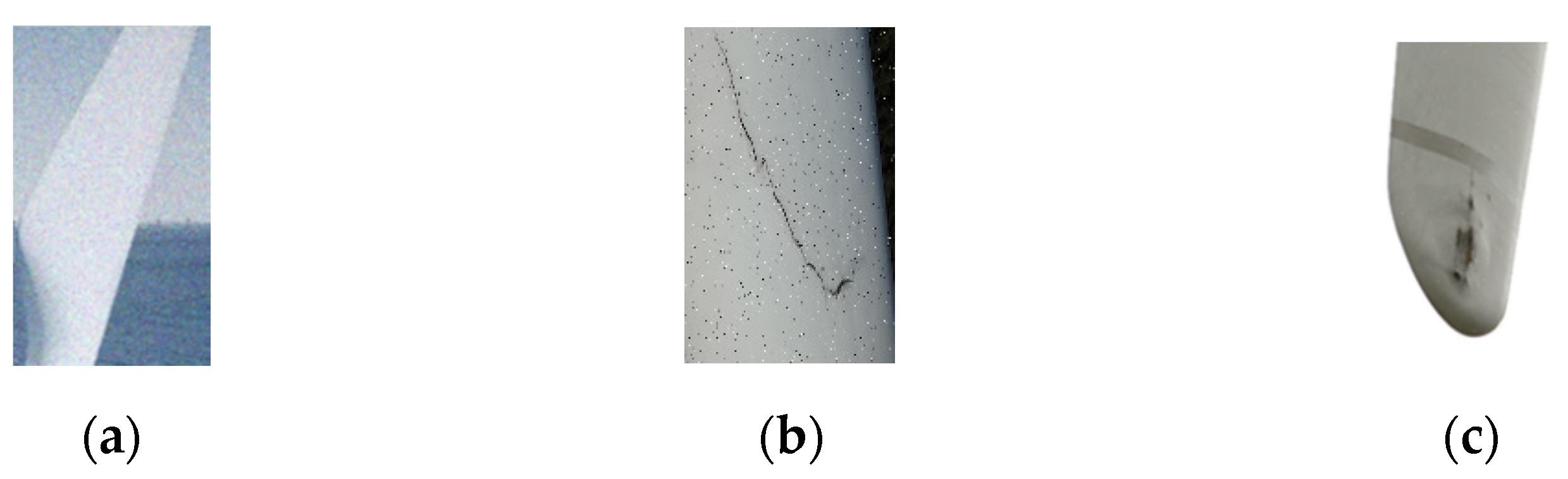
3.2. Wind Turbine Blade Surface Damage Dataset

In this study, we collected 306 images of wind turbine blade in JPG format and 921 s of video data in MOV format from a wind farm using a UAV. After splitting the video data into image data, there are 4396 images in total. The input image size required by ED Net is 56 × 56 pixels, while the image size captured by the UAV is 5472 × 3684 pixels. The captured images are larger in pixels and can be appropriately cropped using OpenCV. When the captured images are not cropped to meet the requirements or have no major features, they can then be appropriately modified manually and cropped to a small 56 × 56 image to meet the input requirements of the network. Then, we performed data augmentation on the dataset by adding random noise, image flipping, and clockwise rotation to the damaged images using OpenCV. After data augmentation, the entire dataset had 2648 images. Lastly, since the color of the image in this experiment has little impact on the identification of damage types, the dataset can be grayed to preserve the gradient, reduce the number of calculations, and accelerate the training speed. The pre-process is shown in Figure 8.
It is categorized according to the type of damage, including normal, cracks, and surface shedding images, as shown in Figure 9. Among them, there are 600 normal pictures, 1008 pictures with cracks, and 1040 pictures with surface shedding.
To mitigate overfitting as much as possible, the training and test sets were divided into 9:1 ratio before the experiment. Before training the network, the dataset was normalized to 56 × 56 and batch normalization was performed to conform the image data to the standard normal distribution and accelerate the model’s convergence rate.

3.3. Model Evaluation Metrics

For the surface damage identification of wind turbine blades in this subject, the optional evaluation metrics include accuracy, precision, recall, and F1 score.

3.3.1. Accuracy

The accuracy is calculated by dividing the number of correctly identified samples by the number of all samples. It is expressed as:
A c c u r a c y = T h e   n u m b e r   o f   c o r r e c t l y   i d e n t i f i e d   s a m p l e s T h e   n u m b e r   o f   a l l   s a m p l e s
Although accuracy can reflect the overall performance of the identification network, it cannot be used as a good metric to measure the results in the case of unbalanced samples. Therefore, other metrics are needed to jointly conduct the experimental evaluation.

3.3.2. Recall, Precision, and F1 Score

There are three types of damage in this work, including cracks, surface shedding, and normal. Therefore, in the confusion matrix for the surface damage of the wind turbine blade, each column represents a type of damage, each row represents the prediction results of each type, and the sum of the data in each row is the real sample number of this type. Therefore, the basic form of the surface damage confusion matrix of the wind turbine can be obtained, as shown in Table 1.
The recall refers to the original sample, which means the probability of being recognized as a positive sample in the actual positive sample. Taking the recall rate of the cracks label as an example, it is shown as:
r = a a + b + c
The precision refers to the recognition results. It means the probability of actually positive samples among all identified positive samples. Taking the precision of crack label as an example, its calculation is shown as:
p = a a + a + a
From the standpoint of identification, recall and precision are incompatible. If the ability to identify models remains unchanged, increasing recall will decrease precision and vice versa.
The F1 score is an evaluation metric that combines the previous two and is used to comprehensively represent the model’s overall evaluation metrics. The formula is as follows:
F = p × r × 2 p + r
Similarly, the accuracy, recall, and F1 score of the wind turbine blade surface shedding damage and normal identification can be calculated. Finally, using macro-averaging, the overall evaluation index of the network model is derived, as shown in Equations (13)–(15).
p _ A vg = p c r a c k s + p S u r f a c e   s h e d d i n g + p N o r m a l 3
r _ A vg = r c a r k s + r S u r f a c e   s h e d d i n g + r N o r m a l 3
F _ A vg = F c r a k s + F S u r f a c e   s h e d d i n g + F N o r m a l 3

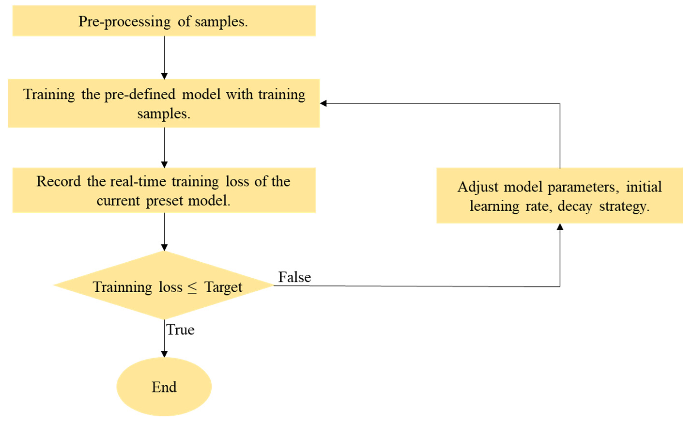
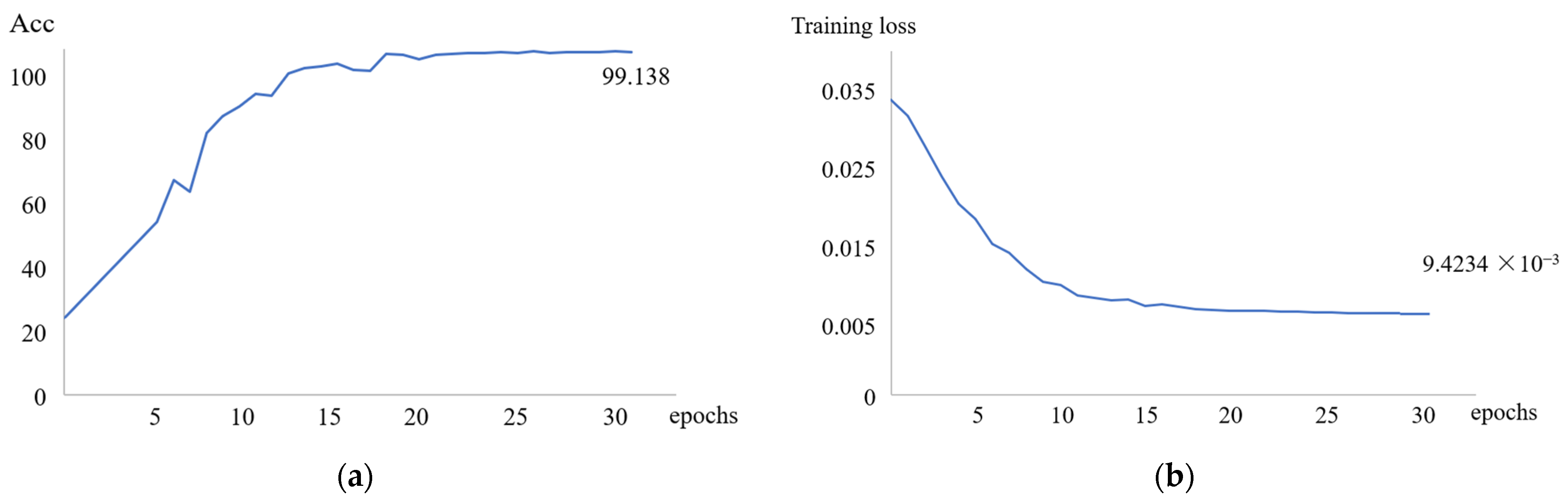
3.4. Training of ED Net

Cross entropy improved by label smoothing is used as the loss function during the training of the ED Net model. Adam gradient descent optimizer with good performance is used for optimization, attenuation rate β 1 = 0.9, β 2 = 0.999 [30], the batch size is set to 32, and the learning rate attenuation strategy with fixed step size is implemented. The initial learning rate is set to 0.001, and it is decreased to 0.6 times the current rate after every 10 epochs. As shown in Figure 10, a total of 30 epochs are trained, and each epoch is trained to record the accuracy and degree of loss of the current model.
The convergence of accuracy and loss of the ED Net model during training is shown in Figure 9 as the number of training epochs increases. During the first 10 training epochs, the accuracy increased and the loss of the model decreased rapidly. Between 11 and 20 training epochs, there is a slight fluctuation in accuracy and a brief plateau in the loss. Possibly, the learning rate of the model during training at this stage is too high; therefore, it is necessary to adjust the learning rate to improve training performance. During the 20-round training period, the learning rate slows for a second time, and the model’s accuracy shows a slow and steady increase, eventually converging at 99.138%. The degree of loss also exhibits a gradual downward trend, eventually converging to 9.4234 ×10⁻³. ED Net is effective at identifying the surface damage of wind turbine blades, according to the convergence of the final model.
It is worthy of discussion that the middle portion of ED Net’s structure can be viewed as a tandem of identical synthetic structures. To investigate the impact of the number of synthetic structures in series on ED Net, a set of ED Net with varying numbers of synthetic structures is designed, as shown in Figure 11. Several experiments are conducted and recorded with the different number of series set to F; the outcomes are shown in Table 2.
According to the experimental results presented in Table 2, the model’s accuracy, recall, precision, and F1 score are all best when F equals 3. When F is greater than 3, the indexes are in an ascending and descending range and are all smaller than when F is equal to 3. We investigate the cause of this phenomenon: the wind turbine blade damage dataset contains small images. Although the small size of the input images can reduce the computational effort of the model after the model continuously downsamples the feature maps, the size and resolution of the feature maps in the model’s depth will be significantly reduced. Consequently, the deeper convolutional layers are unable to extract more effective feature information. Increasing the number of tandem synthetic structures is one of the reasons for this, but the accuracy cannot be improved effectively.

3.5. Validation Experiments on the Effectiveness of Improvements

Because the EAC Block and DPCI_SE Block proposed in this paper are enhanced versions of the AC Block and SE Block, the validity of the enhancement must be confirmed.
To verify the validity of the EAC Block proposed in this paper, a pair of CNNs are developed, with the only structural difference between the EAC Block and AC Block. Similarly, to verify the validity of the DPCI SE Block proposed in this paper, another pair of CNNs models is developed, with the only structural difference between the DPCI_SE Block and the SE Block. We trained and tested these two CNN pairs repeatedly, and the final results are averaged. The structure of the four CNNs is shown in Figure A1.
Table 3 displays four experimental results in total. In terms of accuracy analysis, both the EAC Block and the DPCI_SE Block have an improvement effect, with the EAC Block improving by 0.35% over the AC Block and the DPCI_SE Block improving by 2.05% over the SE Block. In the recall analysis, the EAC Block outperformed the AC Block by 0.45%, while the DPCI_SE Block outperformed the SE Block by 1.59%, indicating that, for identifying complex wind turbine blade damage features, the method of enhancing effective information and suppressing invalid information by enriching spatial location information is more effective than the method of increasing the weight of convolutional kernel skeleton locations. In conjunction with the analysis of the parameter volume, the EAC Block increases the number of parameters more than the DPCI_SE Block, but the enhancement effect on the accuracy and F1 score is not as good as the DPCI_SE Block, indicating that the EAC Block’s enhancement efficiency is inferior to that of the DPCI_SE Block and that further improvement is required. Li Y., Sun M., and Qi Y. [31] use asymmetric convolution to enhance depthwise separable convolution for pest classification. Their ideas inspired us to improve the EAC block with lighter technologies that work better. Nonetheless, the overall increase in the number of parameters introduced by both modules falls within an acceptable range.
Furthermore, it is important to note that the DPCI_SE Block structure is similar to the CAM structure in CBAM [32]. In CAM, the feature map first traverses the dual pooling parallel structure, then the MLP, and then the summation operation. In contrast, in DPCI_SE Block the feature map is fed into the SE block after passing through the dual pooling parallel structure and the splicing operation. We attempt to replace the DPCI SE Block in ED Net with CAM and conduct multiple experiments to determine the mean value; the resulting data are presented in Table 4.
According to experimental results, for the wind turbine blade damage dataset, the number of parameters of CAM is less than that of the DPCI_SE block, but the accuracy rate is slightly lower than that of the DPCI_SE block, which is rich in fine texture features and requires classification of pictures at the pixel level. Therefore, the required number of features is substantial, and the number of channels in the expanded feature map is crucial. This could be one of the reasons why concat is more efficient than add.

3.6. Transfer Learning Experiments

Transfer learning is the reuse of a previously trained model for a different task. In light of the fact that the ED Net model has fewer parameters and is a lightweight CNN model, comparable models include MobileNet_V1 [33], MobileNet_V2 [34], 1.0-SqueezeNext-23 [35], ShuffleNet_V1 [36], and ShuffleNet_V2 [37]. Figure A2 shows their respective primary building blocks and overall structures.
The five pre-trained models are developed experimentally to perform migration learning on the wind turbine blade damage dataset. Each model is trained for 30 epochs, and the final accuracy and training time were recorded. Experiments are conducted with g = 3 because the accuracy of ShuffleNet_V1 is balanced concerning the number of parameters when the number of groups is equal to 3. The experimental result is in Table 5.
As could be seen from Table 5, in terms of accuracy, recall, precision, and F1 index, the ED Net proposed in this paper outperforms the MobileNet_V1, MobileNet_V2, SqueezeNext-23, and ShuffleNet_V1 models on the wind turbine blade damage dataset. MobileNet-V1 and MobileNet_V2 have a greater number of parameters than ED Net. Therefore, the ED Net model can partially replace both of them in the identification of wind turbine blade damage. The first four metrics of the 1.0-SqueezeNext-23 model are inferior to those of the ED Net model, but the model has a small number of parameters and a remarkable training time. ShuffleNet_V2 has slightly higher accuracy than ED Net, a smaller number of parameters, and a shorter training time, which indicates the drawback of the proposed model: the number of parameters is slightly higher than the mainstream lightweight model. In addition, the training time still needs to be improved compared to the broad learning system model [38].
This motivates us to implement the improved method of depthwise separable convolution with channel re-shuffling in our future research to reduce the number of parameters and computations of ED Net. However, ShuffleNet_V2’s recall is slightly lower than that of ED Net. In a real task scenario, our goal is to identify all turbine blades with damage. Therefore, we prefer to implement a small number of manual inspections rather than miss every damaged feature of a wind turbine blade. Consequently, ED Net’s higher recall is an advantage. To sum up, the ED Net model proposed in this paper balances the accuracy with the number of parameters and training time. Under the condition of high accuracy, the number of parameters and training time is still at an average level.

4. Conclusions

Damage identification is of great importance for the maintenance of the wind turbine blade. Observation under weather, light, angle, and other external interference conditions make it difficult to distinguish minute differences in the characteristics of damage to wind turbine blades. In this paper, an improved ED Net model based on the CNN model is proposed to address the issues in the current damage identification methods of the wind turbine blade. It balances cost, complexity, and accuracy by introducing an improved EAC block based on asymmetric convolution and an improved DPCI_SE block based on the SE block.
EAC Block highlights the main feature information obtained by convolution by increasing the weight of the convolution kernel backbone position in the convolution process and further improves the nonlinearity of the convolution module by adding a convolution layer with a convolution kernel of 1 before the convolution branch. DPCI_SE Block primarily enriches the spatial information of features by adding parallel structures of average pooling and maximum pooling before the SE block so that the SE block can enhance the effective feature information and suppress the ineffective or weak feature information to a greater extent.
In this paper, three sets of experiments are conducted. Experiment 1 confirmed the efficacy of the ED Net model for identifying damaged wind turbine blades. Experiment 2 confirmed the efficacy of the relevant enhancements proposed in this work. In addition, based on the analysis of experimental data, the enhancement efficiency of EAC Block is insufficient and requires further development. Experiment 3 compares the damage identification of wind turbine blades by commonly used lightweight networks and demonstrates that the ED Net model proposed in this paper provides superior overall performance. Experiments results show that the ED Net model has an accuracy range of 99.12% to 99.23% and a recall of 99.23%, which can be applied to actual work scenarios. Future research will investigate the light-weighting of ED Net using techniques such as deep separable convolution.

Author Contributions

Conceptualization, H.C.; methodology, H.C.; validation, L.Z.; formal analysis, L.Z.; investigation, H.C.; resources, H.C.; data curation, H.C.; writing—original draft preparation, L.Z. and H.C.; writing—review and editing, L.Z.; supervision, L.Z.; project administration, L.Z.; funding acquisition, L.Z. All authors have read and agreed to the published version of the manuscript.

Funding

This research was funded by the National Natural Science Foundation of China under Grant 52005071 and the Liaoning Provincial Educational Department Project under Grant JDL2020004.

Institutional Review Board Statement

Not applicable.

Informed Consent Statement

Not applicable.

Data Availability Statement

The datasets analyzed during the current study are available from the corresponding author upon reasonable request. The data that support the findings of this study are openly available in “Wind-turbine-blade” at https://github.com/KaKoYu007/Wind-turbine-blade, accessed on 10 April 2022.

Conflicts of Interest

The authors declare no conflict of interest.

Appendix A

Figure A1. Structure of the four CNNs. (a) Structure of EAC block network; (b) structure of AC block network; (c) structure of DPIC_SE block network; (d) structure of SE block network.
Applsci 12 09338 g0a1
Figure A2. Structure of the main building blocks and overall structure of common lightweight CNNs. (a) Structure of MobileNet_V1; (b) structure of MobileNet_V2; (c) structure of ShuffleNet_V1; (d) structure of ShuffleNet_V2; (e) structure of 1.0-SqueezeNext-23.
Applsci 12 09338 g0a2aApplsci 12 09338 g0a2bApplsci 12 09338 g0a2c

References

  1. Balali, M.H.; Nouri, N.; Omrani, E.; Nasiri, A.; Otieno, W. An overview of the environmental, economic, and material developments of the solar and wind sources coupled with the energy storage systems. Int. J. Energy Res. 2017, 41, 1948–1962. [Google Scholar] [CrossRef]
  2. Østergaard, P.A.; Duic, N.; Noorollahi, Y.; Mikulcic, H.; Kalogirou, S. Sustainable development using renewable energy technology. Renew. Energy 2020, 146, 2430–2437. [Google Scholar] [CrossRef]
  3. Azam, A.; Ahmed, A.; Wang, H.; Wang, Y.; Zhang, Z. Knowledge structure and research progress in wind power generation (WPG) from 2005 to 2020 using CiteSpace based scientometric analysis. J. Clean. Prod. 2021, 295, 126496. [Google Scholar] [CrossRef]
  4. Ribrant, J.; Bertling, L. Survey of Failures in Wind Power Systems with Focus on Swedish Wind Power Plants during 1997–2005. In Proceedings of the IEEE Transactions on Energy Conversion, Tampa, FL, USA, 24–28 June 2007; Volume 22, pp. 167–173. [Google Scholar]
  5. Shohag, M.A.; Ndebele, T.; Okoli, O. Real-time damage monitoring in trailing edge bondlines of wind turbine blades with triboluminescent sensors. Struct. Health Monit. 2019, 18, 1129–1140. [Google Scholar] [CrossRef]
  6. Jensen, F.; Terlau, M.; Sorg, M.; Fischer, A. Active Thermography for the Detection of Sub-Surface Defects on a Curved and Coated GFRP-Structure. Appl. Sci. 2022, 11, 9545. [Google Scholar] [CrossRef]
  7. Li, Z.; Tokhi, M.O.; Marks, R.; Zheng, H.; Zhao, Z. Dynamic Wind Turbine Blade Inspection Using Micro-Polarisation Spatial Phase Shift Digital Shearography. Appl. Sci. 2021, 11, 10700. [Google Scholar] [CrossRef]
  8. Aizawa, K.; Poozesh, P.; Niezrecki, C.; Baqersad, J.; Inalpolat, M.; Heilmann, G. An acoustic-array based structural health monitoring technique for wind turbine blades. In Proceedings of the SPIE—The International Society for Optical Engineering, San Diego, CA, USA, 8–12 March 2015; Volume 9437. [Google Scholar]
  9. Joshuva, A.; Sivakumar, S.; Sathishkumar, R.; Deenadayalan, G.; Vishnuvardhan, R. Fault Diagnosis of Wind Turbine Blades using Histogram Features through Nested Dichotomy Classifiers. Int. J. Recent Technol. Eng. 2019, 8, 193–201. [Google Scholar]
  10. Jaramillo, F.; Gutiérrez, J.M.; Orchard, M.; Guarini, M.; Astroza, R. A Bayesian approach for fatigue damage diagnosis and prognosis of wind turbine blades. Mech. Syst. Signal Processing 2022, 174, 109067–109068. [Google Scholar] [CrossRef]
  11. Chandrasekhar, K.; Stevanovic, N.; Cross, E.J.; Dervilis, N.; Worden, K. Damage detection in operational wind turbine blades using a new approach based on machine learning. Renew. Energy 2021, 168, 1249–1264. [Google Scholar] [CrossRef]
  12. Wang, L.; Zhang, Z. Automatic detection of wind turbine blade surface cracks based on UAV-taken images. IEEE Trans. Ind. Electron. 2017, 64, 7293–7303. [Google Scholar] [CrossRef]
  13. Fan, L.; Hu, H.; Zhang, X.; Wang, H.; Kang, C. Magnetic Anomaly Detection Using One-Dimensional Convolutional Neural Network with Multi-Feature Fusion. IEEE Sens. J. 2022, 22, 11637–11643. [Google Scholar] [CrossRef]
  14. Wang, L.; Song, W.; Lan, Y.; Wang, H.; Yue, X.; Yin, X.; Luo, E.; Zhang, B.; Lu, Y.; Tang, Y. A Smart Droplet Detection Approach with Vision Sensing Technique for Agricultural Aviation Application. IEEE Sens. J. 2021, 21, 17508–17516. [Google Scholar] [CrossRef]
  15. Nho, Y.H.; Ryu, S.; Kwon, D.S. UI-GAN: Generative Adversarial Network-Based Anomaly Detection Using User Initial Information for Wearable Devices. IEEE Sens. J. 2021, 21, 9949–9958. [Google Scholar] [CrossRef]
  16. Reddy, A.; Indragandhi, V.; Ravi, L.; Subramaniyaswamy, V. Detection of Cracks and damage in wind turbine blades using artificial intelligence-based image analytics. Measurement 2019, 147, 106823. [Google Scholar] [CrossRef]
  17. Juhi, P.; Sharma, L.; Dhiman, H.S. Wind Turbine Blade Surface Damage Detection based on Aerial Imagery and VGG16-RCNN Framework. arXiv 2021, arXiv:2108.08636. [Google Scholar]
  18. Zhang, J.; Cosma, G.; Watkins, J. Image Enhanced Mask R-CNN: A Deep Learning Pipeline with New Evaluation Measures for Wind Turbine Blade Defect Detection and Classification. J. Imaging 2021, 7, 46. [Google Scholar] [CrossRef] [PubMed]
  19. Zhu, J.; Wen, C.; Liu, J. Defect identification of wind turbine blade based on multi-feature fusion residual network and transfer learning. Energy Sci. Eng. 2021, 10, 219–229. [Google Scholar] [CrossRef]
  20. Sarkar, D.; Gunturi, S.K. Wind turbine blade structural state evaluation by hybrid object detector relying on deep learning models. J. Ambient. Intell. Humaniz. Comput. 2020, 12, 8535–8548. [Google Scholar] [CrossRef]
  21. Zhang, Z.; Fan, B.; Liu, Y.; Zhang, P.; Wang, J.; Du, W. Rapid warning of wind turbine blade icing based on MIV-tSNE-RNN. J. Mech. Sci. Technol. 2021, 35, 5453–5459. [Google Scholar] [CrossRef]
  22. Rezamand, M.; Kordestani, M.; Carriveau, R.; Ting, D.S.K.; Saif, M. A New Hybrid Fault Detection Method for Wind Turbine Blades Using Recursive PCA and Wavelet-Based PDF. IEEE Sens. J. 2020, 20, 2023–2033. [Google Scholar] [CrossRef]
  23. Hu, J.; Shen, L.; Sun, G. Squeeze-and-Excitation Networks. In Proceedings of the 2018 IEEE/CVF Conference on Computer Vision and Pattern Recognition, Salt Lake City, UT, USA, 18–23 June 2018. [Google Scholar]
  24. Radanliev, P.; De Roure, D. Review of Algorithms for Artificial Intelligence on Low Memory Devices. IEEE Access 2021, 9, 109986–109993. [Google Scholar] [CrossRef]
  25. Hendrycks, D.; Gimpel, K. Bridging nonlinearities and stochastic regularizers with Gaussian error linear units. arXiv 2016, arXiv:1606.08415. [Google Scholar]
  26. Ding, X.; Guo, Y.; Ding, G.; Han, J. ACNet: Strengthening the Kernel Skeletons for Powerful CNN via Asymmetric Convolution Blocks. In Proceedings of the 2019 IEEE/CVF International Conference on Computer Vision (ICCV), Seoul, Korea, 20–26 October 2019; pp. 1911–1920. [Google Scholar]
  27. Li, X.; Ma, X. Image Semantic Space Segmentation Based on Cascaded Feature Fusion and Asymmetric Convolution Module. Wirel. Commun. Mob. Comput. 2022, 2022. [Google Scholar] [CrossRef]
  28. Hu, L.; Zhang, H.; Wang, Z.; Huang, C.; Zhang, C. Self-supervised monocular depth estimation via asymmetric convolution block. IET Cyber-Syst. Robot. 2022, 4, 131–138. [Google Scholar] [CrossRef]
  29. Mekruksavanich, S.; Hnoohom, N.; Jitpattanakul, A. A Hybrid Deep Residual Network for Efficient Transitional Activity Recognition Based on Wearable Sensors. Appl. Sci. 2022, 12, 4988. [Google Scholar] [CrossRef]
  30. Kingma Diederik, P.; Adam, J.B. A method for stochastic optimization. arXiv 2014, arXiv:1412.6980. [Google Scholar]
  31. Li, Y.; Sun, M.; Qi, Y. Common pests classification based on asymmetric convolution enhance depthwise separable neural network. J. Ambient. Intell. Humaniz. Comput. 2021, 1–9. [Google Scholar] [CrossRef]
  32. Woo, S.; Park, J.; Lee, J.Y.; Kweon, I.S. Cbam: Convolutional block attention module. In Proceedings of the European Conference on Computer Vision (ECCV), Munich, Germany, 8–14 September 2018. [Google Scholar]
  33. Howard, A.G.; Zhu, M.; Chen, B.; Kalenichenko, D.; Wang, W.; Weyand, T.; Andreetto, M.; Adam, H. Mobilenets: Efficient convolutional neural networks for mobile vision applications. arXiv 2017, arXiv:1704.04861. [Google Scholar]
  34. Sandler, M.; Howard, A.; Zhu, M.; Zhmoginov, A.; Chen, L.C. Mobilenetv2: Inverted residuals and linear bottlenecks. In Proceedings of the IEEE conference on computer vision and pattern recognition, Salt Lake City, UT, USA, 18–21 June 2018. [Google Scholar]
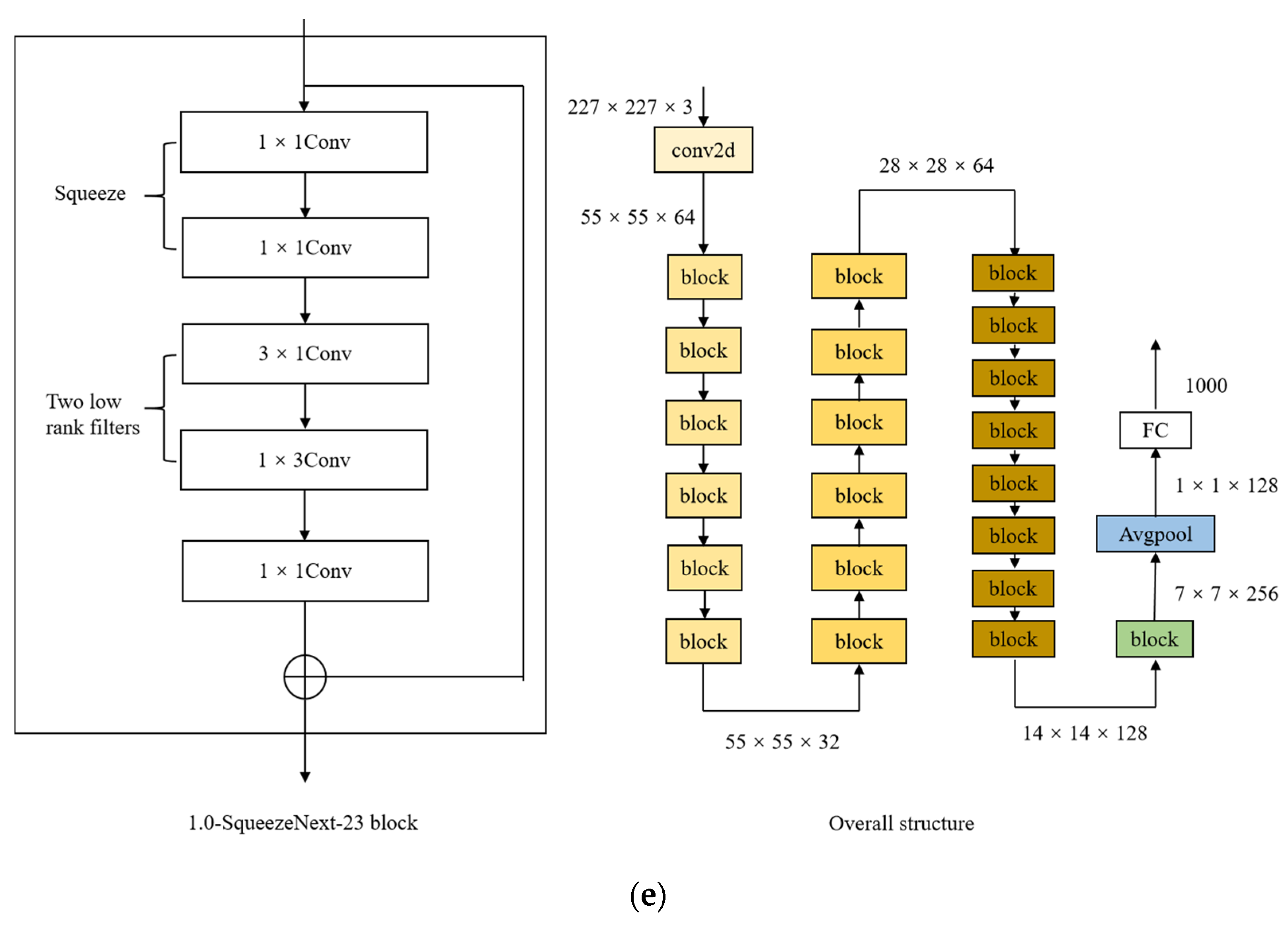
  35. Gholami, A.; Kwon, K.; Wu, B.; Tai, Z.; Yue, X.; Jin, P.; Zhao, S.; Keutzer, K. SqueezeNext: Hardware-Aware Neural Network Design. In Proceedings of the 2018 IEEE/CVF Conference on Computer Vision and Pattern Recognition Workshops (CVPRW), Salt Lake City, UT, USA, 18–22 June 2018. [Google Scholar]
  36. Zhang, X.; Zhou, X.; Lin, M.; Sun, J. ShuffleNet: An Extremely Efficient Convolutional Neural Network for Mobile Devices. In Proceedings of the 2018 IEEE/CVF Conference on Computer Vision and Pattern Recognition, Salt Lake City, UT, USA, 18–23 June 2018. [Google Scholar]
  37. Ma, N.; Zhang, X.; Zheng, H.T.; Sun, J. Shufflenet v2: Practical guidelines for efficient cnn architecture design. In Proceedings of the European conference on computer vision (ECCV), Munich, Germany, 8–14 September 2018. [Google Scholar]
  38. Zou, L.; Wang, Y.; Bi, J.; Sun, Y. Damage Detection in Wind Turbine Blades Based on an Improved Broad Learning System Model. Appl. Sci. 2022, 12, 5164. [Google Scholar] [CrossRef]
Figure 1. Schematic diagram of convolution process.
Applsci 12 09338 g001
Figure 2. The structure of ED Net.
Applsci 12 09338 g002
Figure 3. Flowchart of ED Net training.
Applsci 12 09338 g003
Figure 4. The structure of the skeleton-enhanced kernel.
Applsci 12 09338 g004
Figure 5. After the three convolutional branches extract the features, they are batch-normalized and added together. This operation process is equivalent in effect to a skeleton-enhanced convolution extracting features on the input. Both convolution processes extract a richer feature map.
Applsci 12 09338 g005
Figure 6. The structure of EAC Block.
Applsci 12 09338 g006
Figure 7. The structure of DPCI_SE Block.
Applsci 12 09338 g007
Figure 8. The pre-processing process.
Applsci 12 09338 g008
Figure 9. Three types of wind turbine blade pictures. (a) Normal; (b) cracks; (c) surface shedding.
Applsci 12 09338 g009
Figure 10. (a) The accuracy of ED Net; (b) the training loss of ED Net.
Applsci 12 09338 g010
Figure 11. The structure of a tandem of F synthetic structures.
Applsci 12 09338 g011
Table 1. Confusion matrix for surface damage identification.
LabelIdentified as CracksIdentified as Surface SheddingIdentified as Normal
Cracksab′c′
Surface sheddinga′bc″
Normala″b″c
Table 2. Influence of the number of series connections on ED Net.
FAccuracy/%Recall/%Precision/%F1 ScoreParams/M
297.9197.6397.4997.565.40
399.2399.2699.3599.313.39
499.0298.8698.7398.793.18
598.5198.7298.6598.684.26
699.1698.6699.1398.894.73
798.9398.7198.8998.805.05
Table 3. Comparison results of the four network modules.
ObjectAccuracy/%Recall/%Precision/%F1 ScoreParams/M
CNN By EAC Block95.1294.6995.3695.023.99
CNN By AC Block94.7794.2494.7394.483.08
CNN By DPCI_SE Block97.4297.2697.1197.183.15
CNN By SE Block95.3795.6794.8695.262.87
Table 4. Comparison results of DPCI_SE Block and CAM experiments.
ObjectAccuracy/%Recall/%Precision/%F1 ScoreParams/M
ED Net95.1295.3195.4295.363.99
ED Net(c) 194.7794.5294.2394.373.32
1 Its DPCI_SE Block was replaced by CAM.
Table 5. Comparison of experimental results of common lightweight CNNs.
ObjectAccuracy/%Recall/%Precision/%F1 ScoreParams/MTraining Time
MobileNet_V197.9197.6097.2697.434.2016 min 47 s
MobileNet_V298.5398.6397.7998.213.4016 min 12 s
1.0-SqueezeNext-2393.5992.1492.7092.420.729 min 13 s
ShuffleNet_V1(g = 3)98.5198.4697.5998.022.4016 min 23 s
ShuffleNet_V299.4898.8699.3699.112.315 min 19 s
ED Net99.2399.4399.3499.383.3916 min 06 s
Publisher’s Note: MDPI stays neutral with regard to jurisdictional claims in published maps and institutional affiliations.

