
Enhanced Arabic Sentiment Analysis Using a Novel Stacking Ensemble of Hybrid and Deep Learning Models

 , , , and
Abstract
:1. Introduction
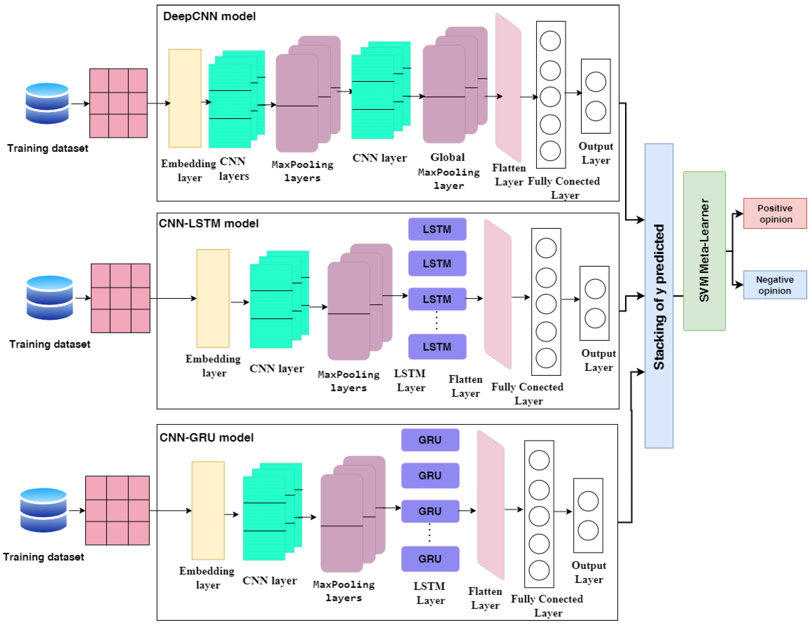
- We proposed three DL architectures: deep convolutional neural network (DeepCNN), hybrid CNN-LSTM, and hybrid CNN-gated recurrent unit (GRU). A Bayesian optimizer has been used to optimize the hyperparameters of these DL models.
- We proposed a heterogeneous ensemble stacking model that combined the three pre-trained DL models of DeepCNN, hybrid CNN-LSTM, and hybrid CNN-GRU. SVM has been used as the meta-learner to combine the outputs of the three base DL models.
- To evaluate the superiority of the proposed ensemble model, the performance of the stacking model has been compared with the performance of several DL and classical ML models using the three well-known Arabic datasets of Arabic health services datasets (Main-AHS and Sub-AHS) and the Arabic sentiment tweets dataset (ASTD).
- The proposed ensemble stacking model significantly outperformed other deep learning models in terms of accuracy, precision, recall, and f1-score.
2. Related Work
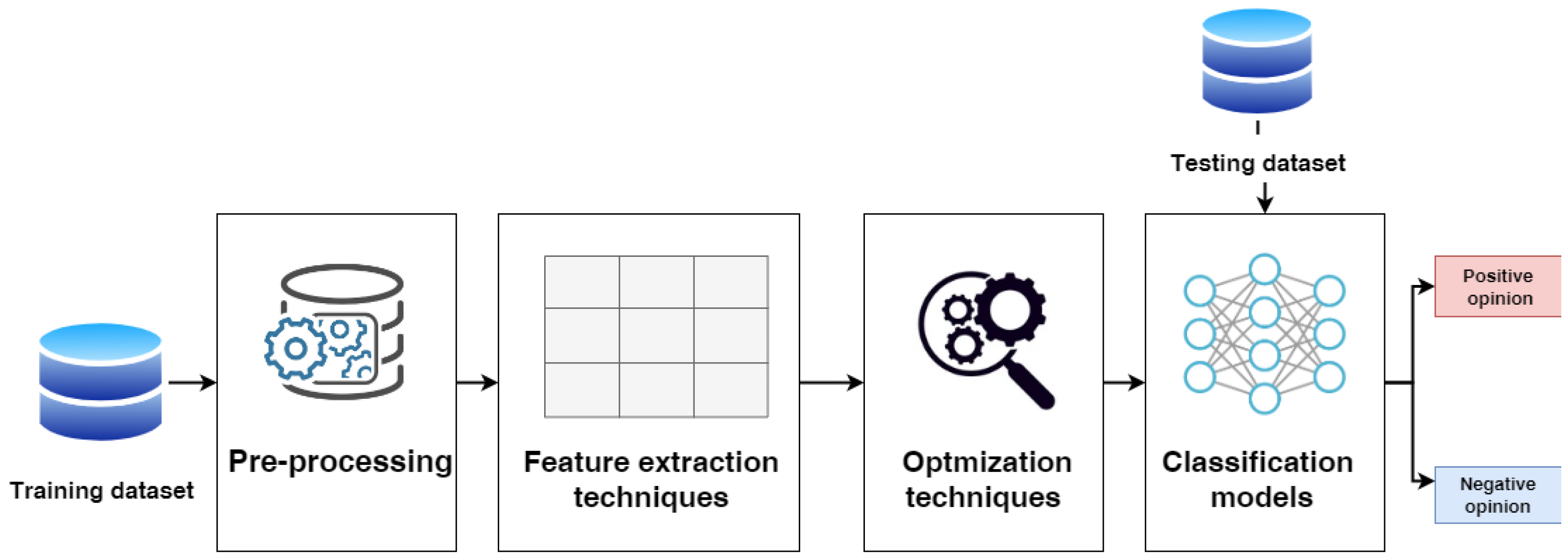
3. Methodology
3.1. Data Pre-Processing
- Cleaning Tweets: this step includes removing HTML tags, URLs, and non-Arabic characters.
- Tokenizing: this step divides the text into parts.
- Pre-processing by removing stop words is a critical step in text pre-processing of sentiment analysis [25,26] because stop words are a collection of words that do not change the meaning of the text or do not hold information, such as prepositions, conjunctions, and articles. Furthermore, they are used to eliminate unimportant words, allowing algorithms to focus on the important words instead. We remove stop words using a stop words list, for example, some words. حيث لدى الا عن ب إلى لنا فقط الذي مثل ذلك
- Stemming: the main job of the stemmer is to return the word to its root.
- Removing emojis.
3.2. Feature Extraction
- For classical ML models, the term frequency/inverse document frequency with N-gram is used to build the feature matrix.
- -
- N-grams are commonly employed in text mining and natural language processing. They are essentially a group of co-occurring words within a particular frame, and computing the n-grams normally moves one word forward, while in more complex cases, it can move N-words forward. N-grams are utilized to keep the context of newly acquired words. It employs a collection of sequentially ordered words based on the value of the N variable. If N = 1, it might be a unigram, and a bigram if N = 2 [27].
- -
- TF-IDF is a statistical measure used to weigh the importance of each word in the corpus. It is a feature extraction method used for classification and recommendation in NLP. The TF-IDF implementation process is divided into two parts. Begin by counting how many times each term appears in the document or tweet. The frequency of each word occurrence (IDF) was then calculated over all papers or tweets. The less important the term, the lower the TF-IDF value. The bigger TF-IDF values, on the other hand, indicate that there are fewer common words in the corpus and therefore are significant [28,29].
- For DL models, word embedding is used to present the word matrix. Word embedding is a method for transforming words in textual input into vectors. It is superior to traditional bag-of-words encoding techniques, which use enormous sparse vectors to encode a whole vocabulary by scoring each word in a vector. The basic idea behind word embedding is that words similar to each other will be adjacent in space. The word’s “embedding” refers to its location in the learned vector space [30]. Word embedding can also be taught as part of a deep learning model, which takes longer but can be customized to a specific training dataset. Each word is represented as a multidimensional unique feature vector in the vector space of a selected dimension in a word embedding. The fundamental idea is to put feature vectors for frequently occurring words in close proximity in space [31]. We used the AraVec word embedding, which is a Python-based open-source project that seeks to provide robust and free word embedding models to the Arabic NLP research community through the usage of the pre-trained distributed word representation. Words are represented in a continuous space as vectors, with numerous syntactic and semantic links encoded between them [32,33]. We used two approaches of AraVec, which are the CBOW and the skip-gram models with 300 dimensions. The CBOW model learns embeddings by predicting the middle word in a sequence based on the words in that sequence, regardless of their order in the sentence. The skip-gram Model seeks to predict the surrounding contextual words given the core word.
3.3. Hyperparameter Optimization
- Grid Search: The hyperparameters’ ideal values are obtained via a tuning procedure. When the Model had several hyperparameters, it became required to search in a multidimensional space for the best combination of values for the hyperparameters [34,35]. Grid search is a hyperparameter tuning method that divides the hyperparameter domain into distinct grids and obtains the optimal combination of hyperparameter values.
- An evaluation method for learning algorithms known as cross-validation separates data into two parts: one for training models while the other is for model verification [36]. Cross-validation includes a single parameter, k, that indicates how many groups a given data sample should be divided into, which is why it is also known as k-fold cross-validation. Cross-validation is seen to be a strong preventive technique against overfitting because the first fold is utilized for the validation set, while the other k-1 folds are provided to the learning system to ensure that the model is estimated using data that were not seen during training [37].
- The KerasTuner hyperparameter optimization system includes the hyperband, Bayesian optimization, and random search algorithms. The optimal hyperparameter values for the models are found by employing one of the search algorithms after the search space is set up using a define-by-run syntax [38]. Hyperparameters are variables that govern the model’s topology and training process and remain constant throughout the training phase, affecting the model’s performance. There are two sorts of hyperparameters: process hyperparameters, which impact the quality and speed of the learning algorithm, and model hyperparameters, which control the number and breadth of hidden layers in the model [39]. For sophisticated models, the number of hyperparameters can be considerably expanded, making manual tuning difficult, and underscoring the need for the techniques. In our work, we optimized some of the values of parameters set for DeepCNN, CNN-LSTM, and CNN-GRU, as shown in Table 1.
3.4. Machine Learning Algorithms
- Logistic regression (LR): Predictions using logistic regression result in discrete values that are best suited for binary categorization. When determining whether or not an event will occur, there are only two options: it will occur or not occur in the binary classifications or even in multi-class classification, and the threshold has to be always specified to distinguish between them [40]. The logistic function (transformation function) or logistic curve (sigmoid curve) is a typical S-shaped curve with the equation, where x is the sigmoid’s midpoint, L is the curve’s peak value, and k is the steepness of the curve or the logistic growth rate. The usual name for the typical logistic function is the sigmoid, which has L = 1, k = 1, and .As a result, an S-curve emerges. The default class is given a set of probabilities as a result of logistic regression different from linear regression, where output is produced straight away. The outcome is between 0 and 1 because it is a probability. The y-value is derived by log converting the x-valueusing the logistic function [41]. After that, a threshold is used to turn the probability into a binary category.
- Naïve Bayes (NB) determines whether the existence of a particular feature in a given class is independent of the existence of any other feature. The Bayes Theorem is used to find the probability of an event occurring in the case that the other event has already occurred [42]. Given our prior knowledge (d), Bayes’ theorem is used to assess the probability of a hypothesis (h) being true:where denotes past probability. = likelihood of data d given data is the prior probability of a class if hypothesis h is true, the chance that hypothesis “h” is right (regardless of the evidence), and is the predictor’s prior probability. Probability of the data (irrespective of the hypothesis). The multinomial model and Bernoulli model are two distinct techniques to build up Naive Bayes [43]. The documents are the classes that are handled as a separate “language” in the multinomial model’s estimate. Bernoulli-NB (Bernoulli Naive Bayes) is a discrete data model that works with occurrence counts and is designed for Boolean/binary characteristics.
- Random forest (RF) takes a group of weak learners and combines them to build a stronger classification predictor [44]. The random forest tree’s main purpose is to use a learning algorithm to merge numerous base-level predictors into a single effective and resilient predictor. In order to classify a new object relying on its attributes, each tree gave a classification and said that the tree “votes” for that class [45]. In the case of regression, the forest picks the category with the most votes (across all forest trees) and takes the average of outputs from different trees. The forest classifiers are fitted using two arrays, one with training data and the other with the goal values of the testing data while creating the random forest tree [46].
- A subset of the supervised learning algorithm family is the Decision Tree (DT) algorithm. A DT is used to develop a training model that can predict the class or value of the target variable by learning fundamental decision rules from prior data, which are the training data. DT has a tree shape structure with internal branches that represent the test outcome, while the leaves or terminal nodes have the class label. The source set is divided into subgroups using an attribute value test, and the result is a trained tree. Recursive partitioning is the process of repeating this action for each derived subset [47].
- KNN is a Supervised ML algorithm [48] which classify data based on similarity through comparing the new case or set of data to the existing cases to place it in the category that is most like the existing categories [49]. As a result, the KNN can swiftly classify new data as it comes in. KNN saves the dataset and then executes an action on it during classification instead of immediately learning from the training set. The KNN approach saves the dataset during the training phase and, when new data is received, classifies it into a category based on the Euclidean distance of the K number of neighbors highly similar to the new data [50].
3.5. Deep Learning Algorithms
- The DeepCNN model includes different layers: the embedding layer, three CNN layers, two MaxPooling layers, Global MaxPooling, flatten, fully connected, and output layers.
- -
- The first layer utilized the embedding layer as a pre-processing step to turn the vector representation into a fixed-sized denser vector representation [51]. It is implemented in the Keras library [52]. Input-dim, output-dim, and input-length are the three parameters that are employed. Input-dim provides the vocabulary size of the dataset, output-dim describes the vector space in which words will be embedded, and input-length describes the length of input sequences. Because both the CBOW and the skip-gram Model are 300 d vectors long, we set the output-dim to 300, the input-dim to 20,000, and the input length to 140.
- -
- The multi-layer neural network known as convolutional neural networks (CNN) is an enhancement of the error backpropagation network [53]. It has a feature map and a convolution filter (kernel). The convolution filter is applied to the input word matrix to create a feature map identifying significant input data patterns. The base of the convolutional operation is the kernel function. Feature extraction is completed by sliding the kernel from top to bottom and from left to right in the input matrix. Each filter also makes use of the rectified linear unit (ReLU) activation function [54] to recognize various aspects of the news.
- -
- The max-pooling layer down samples the feature maps to be more resilient to the probable changes of a feature’s position in the text by recapping the feature’s presence in patches of the feature map. Calculate the maximum value for each feature map patch.
- -
- The two-dimensional arrays of the combined feature maps are flattened into a single, lengthy continuous linear vector using the flatten layer [51].
- -
- The fully connected layer is a dense and deeply connected layer compared to its preceding layer and changes the dimension of the output by implementing a vector-matrix multiplication.
- -
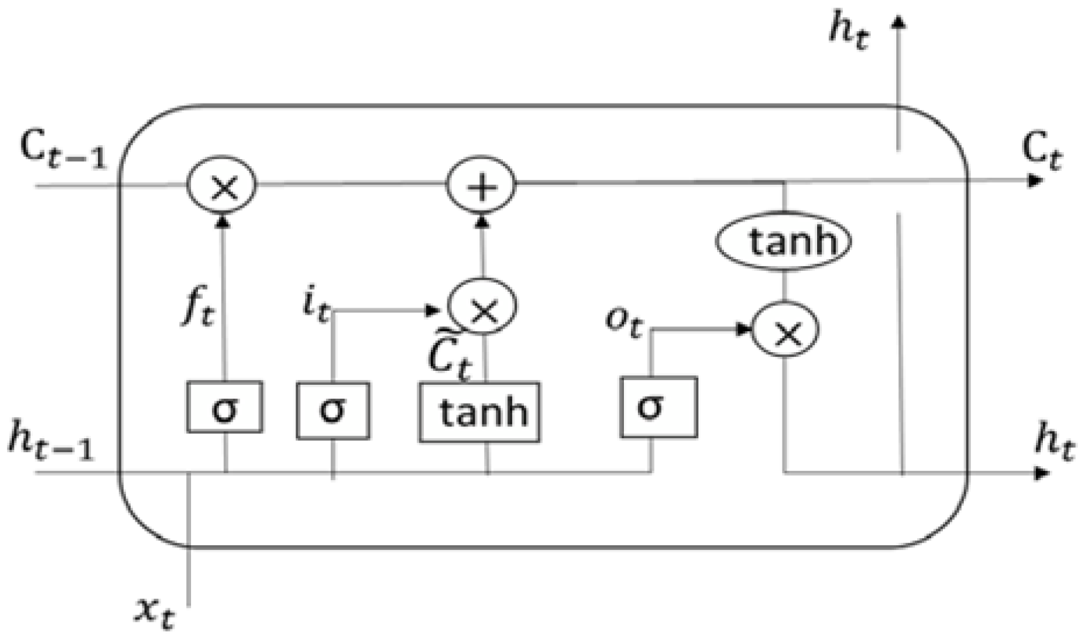
- The embedding layer, CNN and MaxPooling layers, long short-term memory (LSTM), fully linked layer, and output layer are all components that constitute the hybrid CNN-LSTM model.LSTM is a recurrent neural network dependent on DL technology. LSTM is an improved version of RNN that differs from it in one important way: its architecture incorporates a memory cell at the top that allows for efficient information transmission from one instance to the next. In comparison to RNN, it can recall a large amount of information from previous states while avoiding the vanishing gradient problem [57]. By using a novel additive gradient structure that gives direct access to forgotten gate activations, LSTMs are able to tackle the vanishing gradient issue. By often changing the gates at each stage of the learning process, the network may exploit the error gradient to encourage desired behavior. A valve is used to add information to or remove it from the memory cell. The LSTM receives an input from the hidden layer of the current time instance and output from the hidden layer of the prior time instance. These two pieces of data pass via a number of network activation functions and valves before exiting at the output. The LSTM has three gates: an input gate, an output gate, and a forget gate. The forget gate and the input gate, as depicted in Figure 3, select information to be cleaned and appended to the cell state. The cell state can be updated after these two points are known. Finally, the output gate determines the network’s final output [57].
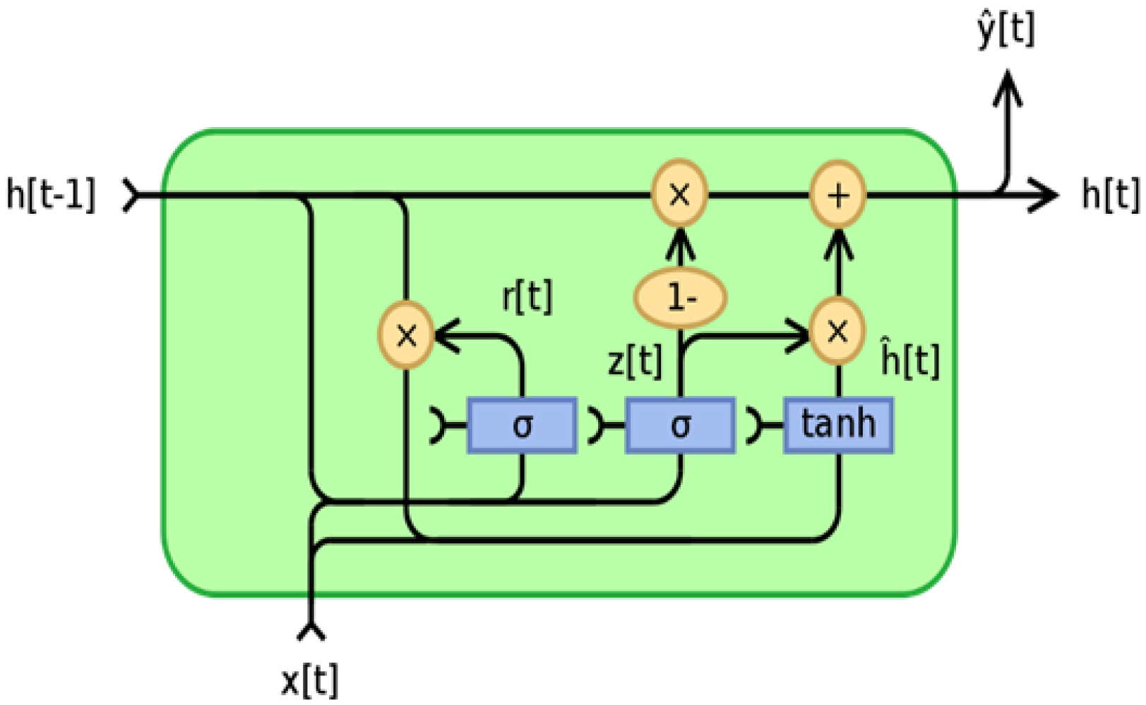
- The hybrid CNN-GRU model includes the embedding layer, CNN layers, MaxPooling layers, gated recurrent unit (GRU), fully connected layer, and output layer. The GRU model is described in detail in the following.GRU was designed to overcome the long-short dependence problem by removing and inflating gradients. As a result, GRU is designed to operate with sequential data that display patterns across time increments, such as time-series data. Because GRU’s architecture is simpler than that of LSTM, its training speed is slightly faster than that of LSTM. The quantity of data that should be added to the next state cell is specified by the update gate. More information is transferred to the next state cell when the update gate value is larger [58]. The reset gate controls how much prior data are deleted. As a result, some information generated in the previous cell may be disregarded or forgotten as the reset gate value changes. Therefore, the update gate is responsible for ensuring that valuable memory is kept so that the next state may be passed on. This is highly beneficial since the model can select duplicating all previous data while avoiding vanishing gradients. The reset gate alters the manner in which new data are stored in previously recorded memory [59]. The GRU operation flow is depicted in Figure 4.
3.6. The Proposed Ensemble Model
- The pre-trained models of DeepCNN, CNN-LSTM, and CNN-GRU that are described in Section 3.5 are loaded, and all layers of the model are frozen without the output layers.
- The output prediction of the training set for each pre-trained model are combined in the training stacking. Then, the stacking is used to train and optimize the meta-learner (SVM in our case). SVM as a meta-learner is optimized using grid search.
- The output predictions of the testing set for each pre-trained model are combined in the testing stacking. Then, the testing stacking is used to evaluate the meta-learner (SVM) using accuracy, precision, recall, f1-score and ROC.
4. Experiments Results
4.1. Datasets
4.1.1. Arabic Health Services Dataset (Main-AHS)
4.1.2. Arabic Health Services Dataset (Sub-AHS Dataset)
4.1.3. Arabic Sentiment Tweets Dataset (ASTD)
4.2. Evaluating Models
4.3. Experimental Setup
4.4. Results
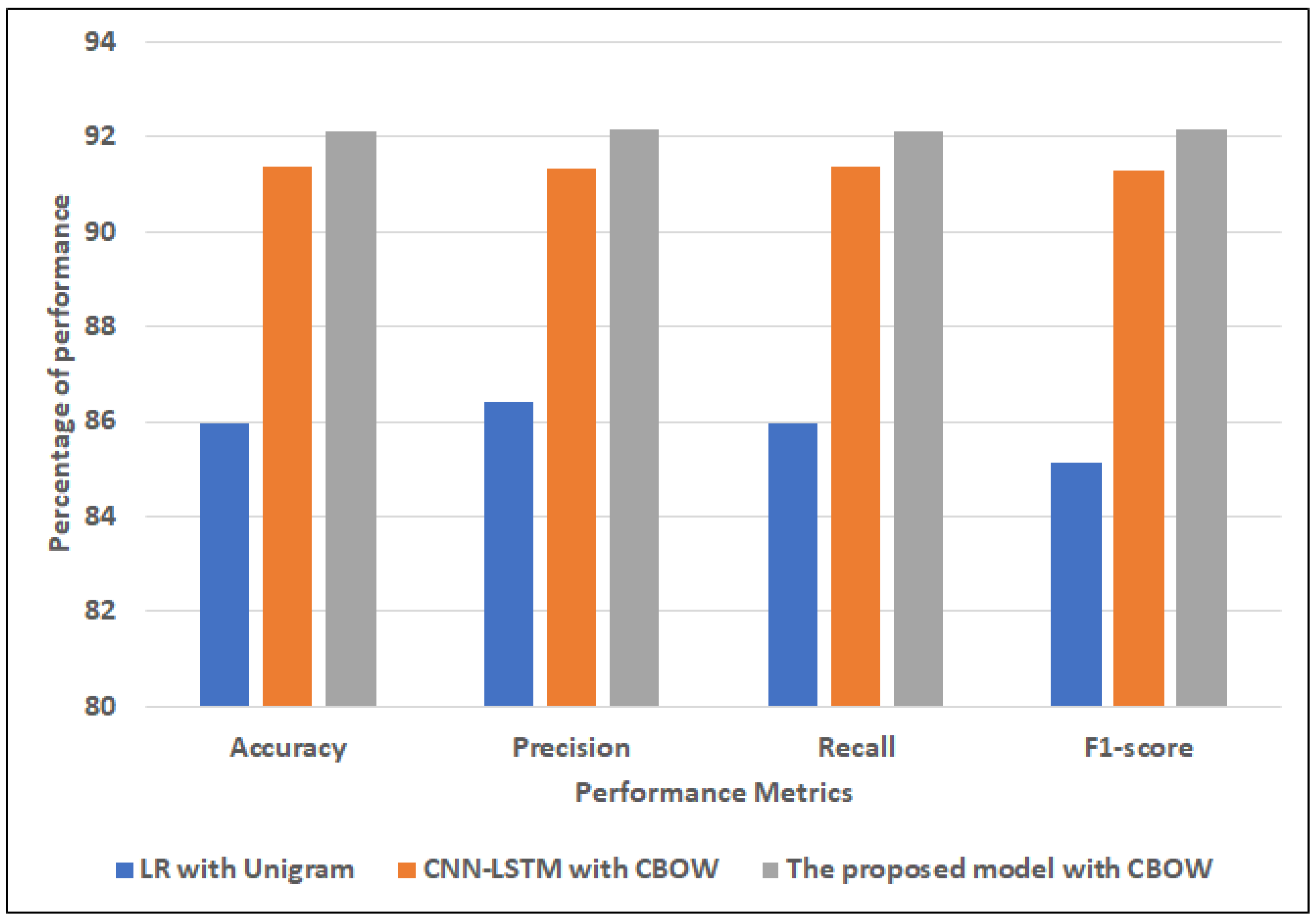
4.4.1. The Performance Results of Models for Main-AHS Dataset
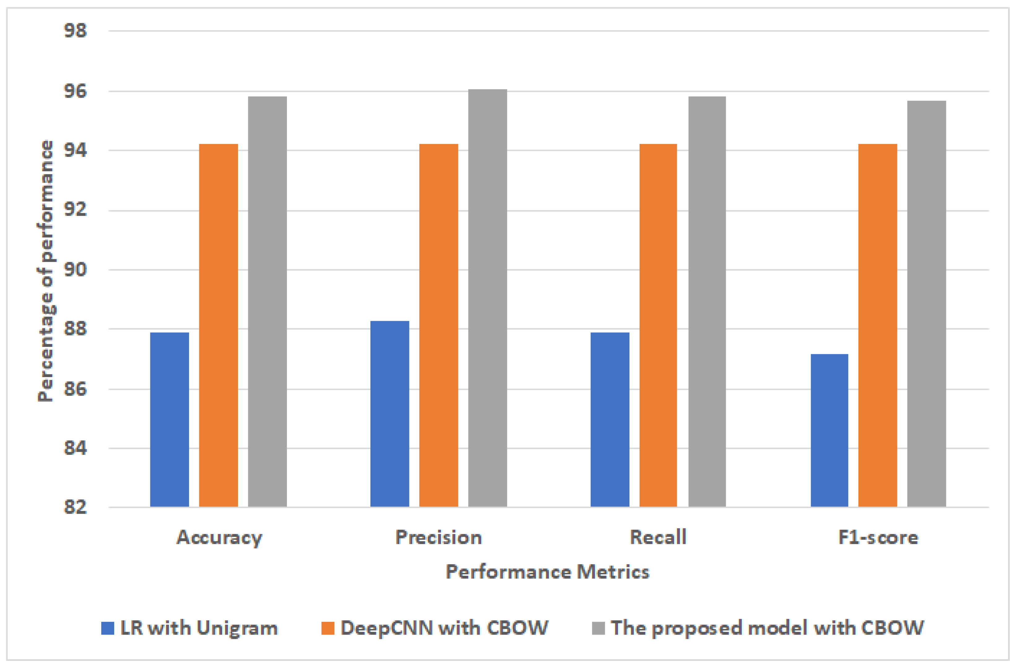
4.4.2. The Performance Results of Models for Sub-AHS Dataset
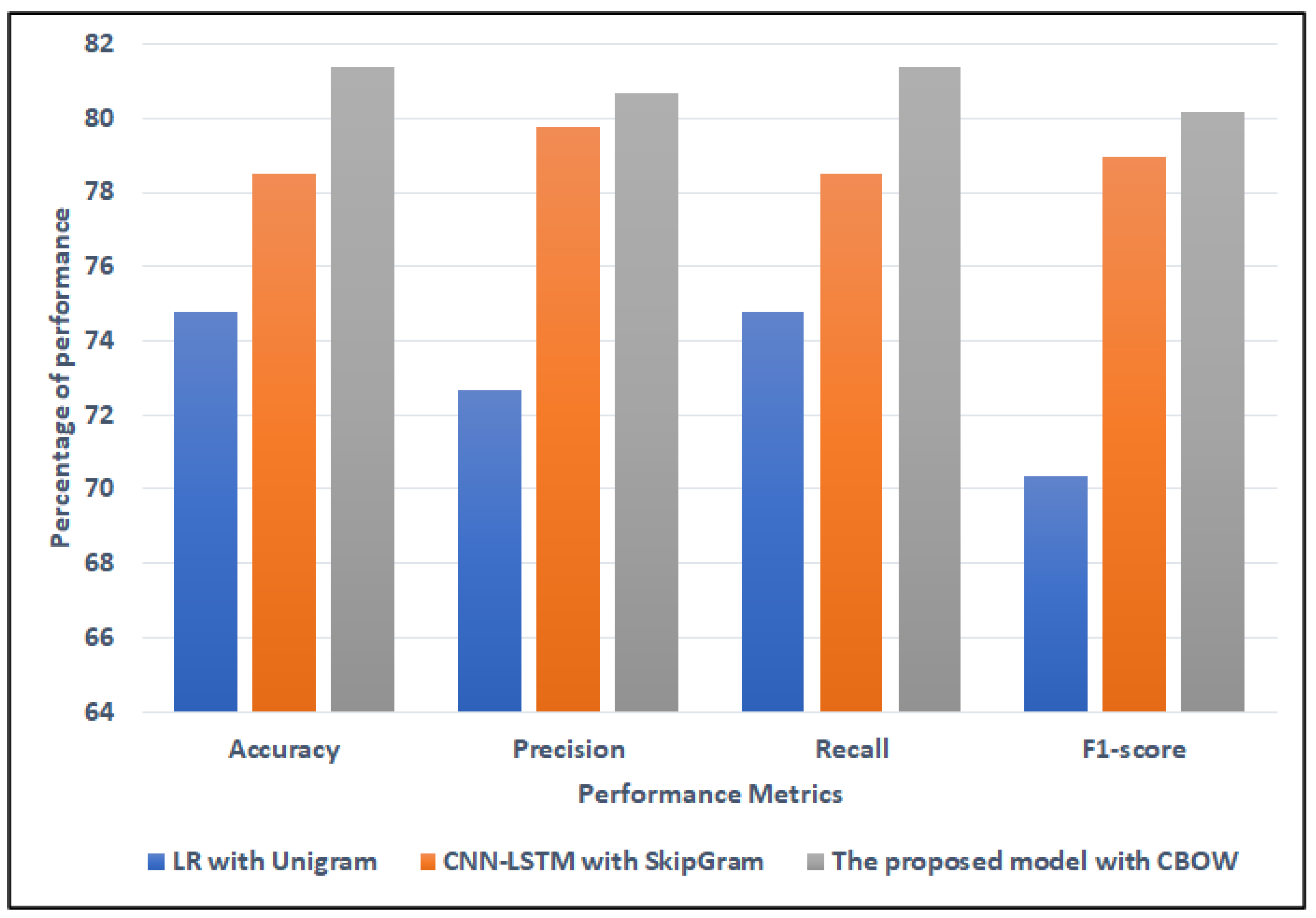
4.4.3. The Performance Results of Models for ASTD Dataset
4.5. Discussion
5. Conclusions
Author Contributions
Funding
Institutional Review Board Statement
Informed Consent Statement
Data Availability Statement
Acknowledgments
Conflicts of Interest
References
- Sosa, P.M. Twitter sentiment analysis using combined LSTM-CNN models. arXiv 2017, arXiv:1807.02911. [Google Scholar]
- El-Affendi, M.A.; Alrajhi, K.; Hussain, A. A novel deep learning-based multilevel parallel attention neural (MPAN) model for multidomain arabic sentiment analysis. IEEE Access 2021, 9, 7508–7518. [Google Scholar] [CrossRef]
- Badaro, G.; Baly, R.; Hajj, H.; El-Hajj, W.; Shaban, K.B.; Habash, N.; Al-Sallab, A.; Hamdi, A. A survey of opinion mining in Arabic: A comprehensive system perspective covering challenges and advances in tools, resources, models, applications, and visualizations. ACM Trans. Asian -Low-Resour. Lang. Inf. Process. 2019, 18, 27. [Google Scholar] [CrossRef]
- Al-Hashedi, A.; Al-Fuhaidi, B.; Mohsen, A.M.; Ali, Y.; Gamal Al-Kaf, H.A.; Al-Sorori, W.; Maqtary, N. Ensemble Classifiers for Arabic Sentiment Analysis of Social Network (Twitter Data) towards COVID-19-Related Conspiracy Theories. Appl. Comput. Intell. Soft Comput. 2022, 2022. [Google Scholar] [CrossRef]
- Zhang, J.; Li, Y.; Tian, J.; Li, T. LSTM-CNN hybrid model for text classification. In Proceedings of the 2018 IEEE 3rd Advanced Information Technology, Electronic and Automation Control Conference (IAEAC), Chongqing, China, 12–14 October 2018; pp. 1675–1680. [Google Scholar]
- Salur, M.U.; Aydin, I. A novel hybrid deep learning model for sentiment classification. IEEE Access 2020, 8, 58080–58093. [Google Scholar] [CrossRef]
- Al Omari, M.; Al-Hajj, M.; Sabra, A.; Hammami, N. Hybrid CNNs-LSTM deep analyzer for arabic opinion mining. In Proceedings of the 2019 Sixth International Conference on Social Networks Analysis, Management and Security (SNAMS), Granada, Spain, 22–25 October 2019; pp. 364–368. [Google Scholar]
- Alwehaibi, A.; Roy, K. Comparison of pre-trained word vectors for arabic text classification using deep learning approach. In Proceedings of the 2018 17th IEEE International Conference on Machine Learning and Applications (ICMLA), Orlando, FL, USA, 17–20 December 2018; pp. 1471–1474. [Google Scholar]
- Heikal, M.; Torki, M.; El-Makky, N. Sentiment analysis of Arabic tweets using deep learning. Procedia Comput. Sci. 2018, 142, 114–122. [Google Scholar] [CrossRef]
- Saleh, H.; Mostafa, S.; Alharbi, A.; El-Sappagh, S.; Alkhalifah, T. Heterogeneous Ensemble Deep Learning Model for Enhanced Arabic Sentiment Analysis. Sensors 2022, 22, 3707. [Google Scholar] [CrossRef]
- Tsoumakas, G.; Partalas, I.; Vlahavas, I. A taxonomy and short review of ensemble selection. In Proceedings of the Workshop on Supervised and Unsupervised Ensemble Methods and Their Applications, Patras, Greece, 21–22 July 2008; pp. 1–6. [Google Scholar]
- Whalen, S.; Pandey, G. A comparative analysis of ensemble classifiers: Case studies in genomics. In Proceedings of the 2013 IEEE 13th International Conference on Data Mining, Dallas, TX, USA, 7–10 December 2013; pp. 807–816. [Google Scholar]
- Sabzevari, M.; Martínez-Muñoz, G.; Suárez, A. Building heterogeneous ensembles by pooling homogeneous ensembles. Int. J. Mach. Learn. Cybern. 2022, 13, 551–558. [Google Scholar] [CrossRef]
- Breiman, L. Bagging predictors. Mach. Learn. 1996, 24, 123–140. [Google Scholar] [CrossRef]
- Svetnik, V.; Wang, T.; Tong, C.; Liaw, A.; Sheridan, R.P.; Song, Q. Boosting: An ensemble learning tool for compound classification and QSAR modeling. J. Chem. Inf. Model. 2005, 45, 786–799. [Google Scholar] [CrossRef]
- Wang, G.; Hao, J.; Ma, J.; Jiang, H. A comparative assessment of ensemble learning for credit scoring. Expert Syst. Appl. 2011, 38, 223–230. [Google Scholar] [CrossRef]
- Farha, I.A.; Magdy, W. Mazajak: An online Arabic sentiment analyser. In Proceedings of the Fourth Arabic Natural Language Processing Workshop, Florence, Italy, 1 August 2019; pp. 192–198. [Google Scholar]
- Dahou, A.; Xiong, S.; Zhou, J.; Haddoud, M.H.; Duan, P. Word embeddings and convolutional neural network for arabic sentiment classification. In Proceedings of the Coling 2016, the 26th International Conference on Computational Linguistics: Technical Papers, Osaka, Japan, 11–16 December 2016; pp. 2418–2427. [Google Scholar]
- Al-Twairesh, N.; Al-Khalifa, H.; Al-Salman, A.; Al-Ohali, Y. Arasenti-tweet: A corpus for arabic sentiment analysis of saudi tweets. Procedia Comput. Sci. 2017, 117, 63–72. [Google Scholar] [CrossRef]
- Omara, E.; Mosa, M.; Ismail, N. Deep convolutional network for arabic sentiment analysis. In Proceedings of the 2018 International Japan-Africa Conference on Electronics, Communications and Computations (JAC-ECC), Alexandria, Egypt, 17–19 December 2018; pp. 155–159. [Google Scholar]
- Elfaik, H. Deep bidirectional lstm network learning-based sentiment analysis for arabic text. J. Intell. Syst. 2021, 30, 395–412. [Google Scholar] [CrossRef]
- Oussous, A.; Lahcen, A.A.; Belfkih, S. Impact of text pre-processing and ensemble learning on Arabic sentiment analysis. In Proceedings of the 2nd International Conference on Networking, Information Systems & Security, Rabat, Morocco, 27–29 March 2019; pp. 1–9. [Google Scholar]
- Kang, M.; Ahn, J.; Lee, K. Opinion mining using ensemble text hidden Markov models for text classification. Expert Syst. Appl. 2018, 94, 218–227. [Google Scholar] [CrossRef]
- Kaddoura, S.; Itani, M.; Roast, C. Analyzing the effect of negation in sentiment polarity of facebook dialectal arabic text. Appl. Sci. 2021, 11, 4768. [Google Scholar] [CrossRef]
- Aldayel, H.K.; Azmi, A.M. Arabic tweets sentiment analysis—A hybrid scheme. J. Inf. Sci. 2016, 42, 782–797. [Google Scholar] [CrossRef]
- Abdulla, N.A.; Ahmed, N.A.; Shehab, M.A.; Al-Ayyoub, M. Arabic sentiment analysis: Lexicon-based and corpus-based. In Proceedings of the 2013 IEEE Jordan Conference on Applied Electrical Engineering and Computing Technologies (AEECT), Amman, Jordan, 3–5 December 2013; pp. 1–6. [Google Scholar]
- Kowsari, K.; Jafari Meimandi, K.; Heidarysafa, M.; Mendu, S.; Barnes, L.; Brown, D. Text classification algorithms: A survey. Information 2019, 10, 150. [Google Scholar] [CrossRef]
- Dhar, A.; Dash, N.S.; Roy, K. Application of tf-idf feature for categorizing documents of online bangla web text corpus. In Intelligent Engineering Informatics; Springer: Berlin/Heidelberg, Germany, 2018; pp. 51–59. [Google Scholar]
- Qaiser, S.; Ali, R. Text mining: Use of TF-IDF to examine the relevance of words to documents. Int. J. Comput. Appl. 2018, 181, 25–29. [Google Scholar] [CrossRef]
- Lai, S.; Liu, K.; He, S.; Zhao, J. How to generate a good word embedding. IEEE Intell. Syst. 2016, 31, 5–14. [Google Scholar] [CrossRef]
- Wang, B.; Wang, A.; Chen, F.; Wang, Y.; Kuo, C.C.J. Evaluating word embedding models: Methods and experimental results. APSIPA Trans. Signal Inf. Process. 2019, 8, e19. [Google Scholar] [CrossRef]
- Soliman, A.B.; Eissa, K.; El-Beltagy, S.R. Aravec: A set of arabic word embedding models for use in arabic nlp. Procedia Comput. Sci. 2017, 117, 256–265. [Google Scholar] [CrossRef]
- Suleiman, D.; Awajan, A.A.; Al Etaiwi, W. Arabic text keywords extraction using word2vec. In Proceedings of the 2019 2nd International Conference on new Trends in Computing Sciences (ICTCS), Amman, Jordan, 9–11 October 2019; pp. 1–7. [Google Scholar]
- Fayed, H.A.; Atiya, A.F. Speed up grid-search for parameter selection of support vector machines. Appl. Soft Comput. 2019, 80, 202–210. [Google Scholar] [CrossRef]
- Pontes, F.J.; Amorim, G.; Balestrassi, P.P.; Paiva, A.; Ferreira, J.R. Design of experiments and focused grid search for neural network parameter optimization. Neurocomputing 2016, 186, 22–34. [Google Scholar] [CrossRef]
- Browne, M.W. Cross-validation methods. J. Math. Psychol. 2000, 44, 108–132. [Google Scholar] [CrossRef] [PubMed]
- Refaeilzadeh, P.; Tang, L.; Liu, H. Cross-validation. Encycl. Database Syst. 2009, 5, 532–538. [Google Scholar]
- O’Malley, T.; Bursztein, E.; Long, J.; Chollet, F.; Jin, H.; Invernizzi, L. Hyperparameter Tuning with Keras Tuner. 2019. Available online: https://github.com/keras-team/keras-tuner (accessed on 23 July 2022).
- Shawki, N.; Nunez, R.R.; Obeid, I.; Picone, J. On Automating Hyperparameter Optimization for Deep Learning Applications. In Proceedings of the 2021 IEEE Signal Processing in Medicine and Biology Symposium (SPMB), Philadelphia, PA, USA, 4 December 2021; pp. 1–7. [Google Scholar]
- Nusinovici, S.; Tham, Y.C.; Yan, M.Y.C.; Ting, D.S.W.; Li, J.; Sabanayagam, C.; Wong, T.Y.; Cheng, C.Y. Logistic regression was as good as machine learning for predicting major chronic diseases. J. Clin. Epidemiol. 2020, 122, 56–69. [Google Scholar] [CrossRef]
- Rymarczyk, T.; Kozłowski, E.; Kłosowski, G.; Niderla, K. Logistic regression for machine learning in process tomography. Sensors 2019, 19, 3400. [Google Scholar] [CrossRef]
- John, G.H.; Langley, P. Estimating continuous distributions in Bayesian classifiers. arXiv 2013, arXiv:1302.4964. [Google Scholar]
- Sarker, I.H. A machine learning based robust prediction model for real-life mobile phone data. Internet Things 2019, 5, 180–193. [Google Scholar] [CrossRef]
- Breiman, L. Random forests. Mach. Learn. 2001, 45, 5–32. [Google Scholar] [CrossRef]
- Sarker, I.H.; Kayes, A.; Watters, P. Effectiveness analysis of machine learning classification models for predicting personalized context-aware smartphone usage. J. Big Data 2019, 6, 57. [Google Scholar] [CrossRef]
- Amit, Y.; Geman, D. Shape quantization and recognition with randomized trees. Neural Comput. 1997, 9, 1545–1588. [Google Scholar] [CrossRef]
- Boehmke, B.; Greenwell, B. Hands-on Machine Learning with R; Chapman and Hall/CRC: Boca Raton, FL, USA, 2019. [Google Scholar]
- Sun, S.; Huang, R. An adaptive k-nearest neighbor algorithm. In Proceedings of the 2010 Seventh International Conference on Fuzzy Systems and Knowledge Discovery, Yantai, China, 10–12 August 2010; Volume 1, pp. 91–94. [Google Scholar]
- Zhang, Z. Introduction to machine learning: K-nearest neighbors. Ann. Transl. Med. 2016, 4, 218. [Google Scholar] [CrossRef] [Green Version]
- Laaksonen, J.; Oja, E. Classification with learning k-nearest neighbors. In Proceedings of the International Conference on Neural Networks (ICNN’96), Washington, DC, USA, 3–6 June 1996; Volume 3, pp. 1480–1483. [Google Scholar]
- Li, Z.; Liu, F.; Yang, W.; Peng, S.; Zhou, J. A survey of convolutional neural networks: Analysis, applications, and prospects. IEEE Trans. Neural Netw. Learn. Syst. 2021. [Google Scholar] [CrossRef] [PubMed]
- Chollet, F. Keras: The Python Deep Learning Library; Astrophysics Source Code Library: Mountain View, CA, USA, 2018. [Google Scholar]
- O’Shea, K.; Nash, R. An introduction to convolutional neural networks. arXiv 2015, arXiv:1511.08458. [Google Scholar]
- Agarap, A.F. Deep learning using rectified linear units (relu). arXiv 2018, arXiv:1803.08375. [Google Scholar]
- Zhang, Z. Improved adam optimizer for deep neural networks. In Proceedings of the 2018 IEEE/ACM 26th International Symposium on Quality of Service (IWQoS), Banff, AB, Canada, 4–6 June 2018; pp. 1–2. [Google Scholar]
- Wanto, A.; Windarto, A.P.; Hartama, D.; Parlina, I. Use of binary sigmoid function and linear identity in artificial neural networks for forecasting population density. Int. J. Inf. Syst. Technol. 2017, 1, 43–54. [Google Scholar] [CrossRef]
- Lipton, Z.C.; Kale, D.C.; Elkan, C.; Wetzel, R. Learning to diagnose with LSTM recurrent neural networks. arXiv 2015, arXiv:1511.03677. [Google Scholar]
- Dey, R.; Salem, F.M. Gate-variants of gated recurrent unit (GRU) neural networks. In Proceedings of the 2017 IEEE 60th International Midwest Symposium on Circuits and Systems (MWSCAS), Boston, MA, USA, 6–9 August 2017; pp. 1597–1600. [Google Scholar]
- Ravanelli, M.; Brakel, P.; Omologo, M.; Bengio, Y. Light gated recurrent units for speech recognition. IEEE Trans. Emerg. Top. Comput. Intell. 2018, 2, 92–102. [Google Scholar] [CrossRef]
- Gruber, N.; Jockisch, A. Are GRU cells more specific and LSTM cells more sensitive in motive classification of text? Front. Artif. Intell. 2020, 3, 40. [Google Scholar] [CrossRef] [PubMed]
- Sagi, O.; Rokach, L. Ensemble learning: A survey. Wiley Interdiscip. Rev. Data Min. Knowl. Discov. 2018, 8, e1249. [Google Scholar] [CrossRef]
- Alayba, A.M.; Palade, V.; England, M.; Iqbal, R. Arabic language sentiment analysis on health services. In Proceedings of the 2017 1st International Workshop on Arabic Script Analysis and Recognition (ASAR), Nancy, France, 3–5 April 2017; pp. 114–118. [Google Scholar]
- Alayba, A.M.; Palade, V.; England, M.; Iqbal, R. Improving sentiment analysis in Arabic using word representation. In Proceedings of the 2018 IEEE 2nd International Workshop on Arabic and Derived Script Analysis and Recognition (ASAR), London, UK, 12–14 March 2018; pp. 13–18. [Google Scholar]
- Nabil, M.; Aly, M.; Atiya, A. Astd: Arabic sentiment tweets dataset. In Proceedings of the 2015 Conference on Empirical Methods in Natural Language Processing, Lisbon, Portugal, 17–21 September 2015; pp. 2515–2519. [Google Scholar]
- Flach, P.A. ROC analysis. In Encyclopedia of Machine Learning and Data Mining; Springer: Berlin/Heidelberg, Germany, 2016; pp. 1–8. [Google Scholar]
- Sokolova, M.; Japkowicz, N.; Szpakowicz, S. Beyond accuracy, F-score and ROC: A family of discriminant measures for performance evaluation. In Lecture Notes in Computer Science: Proceedings of the Australasian Joint Conference on Artificial Intelligence; Springer: Berlin/Heidelberg, Germany, 2006; pp. 1015–1021. [Google Scholar]
- Kaddoura, S.; D. Ahmed, R. A comprehensive review on Arabic word sense disambiguation for natural language processing applications. Wiley Interdiscip. Rev. Data Min. Knowl. Discov. 2022, 12, e1447. [Google Scholar] [CrossRef]


| Parameters | Values |
|---|---|
| Num_filters | [64, 128, 256, 512] |
| Kernel_size | [2, 3, 4, 5] |
| Pool_Size | [2, 3, 4, 5] |
| LSTM_Unit | Range (50, 1000) |
| GRU_Unit | Range (50, 1000) |
| Dense_Unit | Range (50, 1000) |
| learning_rate | Between 1 × and 1 × |
| Models | Parameters | Values for Main-AHS Dataset | Values for Sub-AHS Dataset | Values for ASTD Dataset |
|---|---|---|---|---|
| CNN | Num_filters | [256, 128, 128] | [128, 256, 256] | [256, 128, 128] |
| Kernel_size | [4, 5, 2] | [4, 5, 4] | [3, 5, 4] | |
| Pool_Size | [4, 5, 3] | [2, 4] | [2, 5] | |
| Dense_Unit | 300 | 150 | 500 | |
| learning_rate | 0.0012 | 0.00152 | 0.0007 | |
| CNN-LSTM | Num_filters | 128 | 256 | 256 |
| Kernel_size | 4 | 4 | 3 | |
| Pool_Size | 5 | 2 | 2 | |
| LSTM_Unit | 400 | 500 | 550 | |
| Dense_Unit | 800 | 700 | 300 | |
| learning_rate | 0.0012 | 0.0025 | 0.0046 | |
| CNN-GRU | Num_filters | 256 | 64 | 128 |
| Kernel_size | 5 | 3 | 5 | |
| Pool_Size | 2 | 3 | 2 | |
| GRU_Unit | 950 | 150 | 250 | |
| Dense_Unit | 150 | 900 | 300 | |
| learning_rate | 0.0012 | 0.0059 | 0.0021 |
| Models | Parameters | Values for Main-AHS Dataset | Values for Sub-AHS Dataset | Values for ASTD Dataset |
|---|---|---|---|---|
| CNN | Num_filters | [256, 256, 512] | [128, 128, 500] | [128, 256, 512] |
| Kernel_size | [5, 4, 4] | [5, 5, 5] | [2, 5, 5] | |
| Pool_Size | [2, 4] | [2, 4] | [2, 5] | |
| Dense_Unit | 500 | 300 | 400 | |
| learning_rate | 0.0012 | 0.0014 | 0.00304 | |
| CNN-LSTM | Num_filters | 64 | 512 | 200 |
| Kernel_size | 5 | 5 | 2 | |
| Pool_Size | 3 | 2 | 2 | |
| LSTM_Unit | 200 | 600 | 200 | |
| Dense_Unit | 450 | 680 | 600 | |
| learning_rate | 0.00525 | 0.00051 | 0.0007 | |
| CNN-GRU | Num_filters | 64 | 64 | 128 |
| Kernel_size | 3 | 5 | 5 | |
| Pool_Size | 5 | 3 | 4 | |
| GRU_Unit | 350 | 450 | 100 | |
| Dense_Unit | 200 | 870 | 950 | |
| learning_rate | 0.0054 | 0.00142 | 0.0013 |
| Approaches | Models | Feature Extraction Method | Testing Performance | |||
|---|---|---|---|---|---|---|
| Accuracy | Precision | Recall | F1-Score | |||
| ML approach | KNN | Unigram | 82.02 | 83.1 | 82.02 | 80.22 |
| Bi-gram | 68.97 | 47.56 | 68.97 | 56.3 | ||
| DT | Unigram | 79.56 | 79.35 | 79.56 | 79.44 | |
| Bi-gram | 77.09 | 76.25 | 77.09 | 75.25 | ||
| LR | Unigram | 85.96 | 86.41 | 85.96 | 85.13 | |
| Bi-gram | 78.33 | 77.63 | 78.33 | 76.82 | ||
| NB | Unigram | 82.02 | 85.29 | 82.02 | 79.5 | |
| Bi-gram | 82.02 | 82.38 | 82.02 | 80.57 | ||
| RF | Unigram | 83.74 | 84.43 | 83.74 | 82.47 | |
| Bi-gram | 78.08 | 78.32 | 78.08 | 75.53 | ||
| DL approach | Deep CNN | SkipGram | 89.41 | 89.49 | 89.41 | 89.44 |
| CNN-LSTM | 90.38 | 90.36 | 90.38 | 90.37 | ||
| CNN-GRU | 90.89 | 91.08 | 90.89 | 90.95 | ||
| Deep CNN | CBOW | 90.64 | 90.74 | 90.64 | 90.68 | |
| CNN-LSTM | 91.38 | 91.31 | 91.38 | 91.27 | ||
| CNN-GRU | 91.02 | 91.02 | 91.02 | 91.02 | ||
| The proposed ensemble model | Stacking LR | SkipGram | 91.63 | 91.56 | 91.63 | 91.57 |
| Stacking LR | CBOW | 92.12 | 92.16 | 92.12 | 92.14 | |
| Approaches | Models | Feature Extraction Method | Testing Performance | |||
|---|---|---|---|---|---|---|
| Accuracy | Precision | Recall | F1-Score | |||
| ML approach | KNN | Unigram | 79.83 | 82.32 | 79.83 | 76.31 |
| Bi-gram | 70.89 | 50.26 | 70.89 | 58.82 | ||
| DT | Unigram | 83.0 | 82.86 | 83.0 | 82.92 | |
| Bi-gram | 80.12 | 80.04 | 80.12 | 77.97 | ||
| LR | Unigram | 87.9 | 88.29 | 87.9 | 87.19 | |
| Bi-gram | 82.71 | 82.69 | 82.71 | 81.33 | ||
| NB | Unigram | 80.69 | 84.15 | 80.69 | 77.24 | |
| Bi-gram | 83.29 | 83.14 | 83.29 | 82.13 | ||
| RF | Unigram | 86.17 | 86.96 | 86.17 | 85.06 | |
| Bi-gram | 81.56 | 82.1 | 81.56 | 79.5 | ||
| DL approach | Deep CNN | SkipGram | 93.08 | 93.13 | 93.08 | 93.1 |
| CNN-LSTM | 93.66 | 93.61 | 93.66 | 93.6 | ||
| CNN-GRU | 93.20 | 93.30 | 93. 20 | 93.30 | ||
| Deep CNN | CBOW | 94.24 | 94.21 | 94.24 | 94.22 | |
| CNN-LSTM | 93.37 | 93.34 | 93.37 | 93.28 | ||
| CNN-GRU | 93.66 | 93.61 | 93.66 | 93.6 | ||
| The proposed ensemble model | Stacking SVM | SkipGram | 94.95 | 94.9 | 94.95 | 94.9 |
| Stacking SVM | CBOW | 95.81 | 96.06 | 95.81 | 95.67 | |
| Approaches | Models | Feature Extraction Method | Testing Performance | |||
|---|---|---|---|---|---|---|
| Accuracy | Precision | Recall | F1-Score | |||
| ML approach | KNN | Unigram | 71.9 | 51.7 | 71.9 | 60.15 |
| Bi-gram | 71.9 | 51.7 | 71.9 | 60.15 | ||
| DT | Unigram | 56.61 | 63.34 | 56.61 | 58.69 | |
| Bi-gram | 71.9 | 66.43 | 71.9 | 63.46 | ||
| LR | Unigram | 74.79 | 72.65 | 74.79 | 70.35 | |
| Bi-gram | 71.69 | 65.71 | 71.69 | 63.33 | ||
| NB | Unigram | 73.55 | 70.86 | 73.55 | 69.86 | |
| Bi-gram | 72.31 | 68.07 | 72.31 | 63.71 | ||
| RF | Unigram | 64.67 | 64.91 | 64.67 | 64.79 | |
| Bi-gram | 71.9 | 66.36 | 71.9 | 63.17 | ||
| DL approach | Deep CNN | SkipGram | 71.28 | 74.73 | 71.28 | 72.36 |
| CNN-LSTM | 78.51 | 79.75 | 78.51 | 78.97 | ||
| CNN-GRU | 77.69 | 79.5 | 77.69 | 78.29 | ||
| Deep CNN | CBOW | 76.86 | 78.71 | 76.86 | 77.49 | |
| CNN-LSTM | 78.1 | 78.41 | 78.1 | 78.24 | ||
| CNN-GRU | 78.1 | 79.35 | 78.1 | 78.56 | ||
| The proposed ensemble model | Stacking SVM | SkipGram | 80.17 | 79.52 | 80.17 | 79.71 |
| Stacking SVM | CBOW | 81.4 | 80.69 | 81.4 | 80.16 | |
| Paper | Method | Dataset | Performance |
|---|---|---|---|
| [9] | CNN-LSTM | ASTD | 65.05% for accuracy 64.46% for f1-score |
| [17] | CNN-LSTM | ASTD | 66% for accuracy, 62% for f1-score 66% for recall |
| [7] | CNN-LSTM | Main-AHS | 88.1% for accuracy |
| ASTD | 79.18 % for accuracy | ||
| [18] | CNN | ASTD | 79.07% for accuracy |
| [21] | ensemble model using voting based on CNN-LSTM | ASTD | 64.46% for f1-score |
| [63] | Bi-LSTM | ASTD | 79.25% for Accuracy 76.83 of F1-score |
| Main-AHS | 92.61% for Accuracy 86.03% of f1-score | ||
| [9] | CNN | Main-AHS | 92% for accuracy |
| Sub-AHS | 95% for accuracy | ||
| The proposed model | Stacking SVM based on integrated DeepCNN, CNN-LSTM and CNN-GRU | Main-AHS | 92.12% for accuracy 91.31% for precision 91.38% of recall 91.27% of f1-score |
| Sub-AHS | 95.81% for accuracy 96.06% for precision 95.81% for recall 95.67% for f1-score | ||
| ASTD | 81.4% for accuracy 80.69% of precision 81.4% for recall 80% for f1-score |
Publisher’s Note: MDPI stays neutral with regard to jurisdictional claims in published maps and institutional affiliations. |
© 2022 by the authors. Licensee MDPI, Basel, Switzerland. This article is an open access article distributed under the terms and conditions of the Creative Commons Attribution (CC BY) license (https://creativecommons.org/licenses/by/4.0/).
Share and Cite
Saleh, H.; Mostafa, S.; Gabralla, L.A.; O. Aseeri, A.; El-Sappagh, S. Enhanced Arabic Sentiment Analysis Using a Novel Stacking Ensemble of Hybrid and Deep Learning Models. Appl. Sci. 2022, 12, 8967. https://doi.org/10.3390/app12188967
Saleh H, Mostafa S, Gabralla LA, O. Aseeri A, El-Sappagh S. Enhanced Arabic Sentiment Analysis Using a Novel Stacking Ensemble of Hybrid and Deep Learning Models. Applied Sciences. 2022; 12(18):8967. https://doi.org/10.3390/app12188967
Chicago/Turabian StyleSaleh, Hager, Sherif Mostafa, Lubna Abdelkareim Gabralla, Ahmad O. Aseeri, and Shaker El-Sappagh. 2022. "Enhanced Arabic Sentiment Analysis Using a Novel Stacking Ensemble of Hybrid and Deep Learning Models" Applied Sciences 12, no. 18: 8967. https://doi.org/10.3390/app12188967
APA StyleSaleh, H., Mostafa, S., Gabralla, L. A., O. Aseeri, A., & El-Sappagh, S. (2022). Enhanced Arabic Sentiment Analysis Using a Novel Stacking Ensemble of Hybrid and Deep Learning Models. Applied Sciences, 12(18), 8967. https://doi.org/10.3390/app12188967