
Exploiting Hierarchical Label Information in an Attention-Embedding, Multi-Task, Multi-Grained, Network for Scene Classification of Remote Sensing Imagery


Abstract
:1. Introduction
2. Materials and Methods
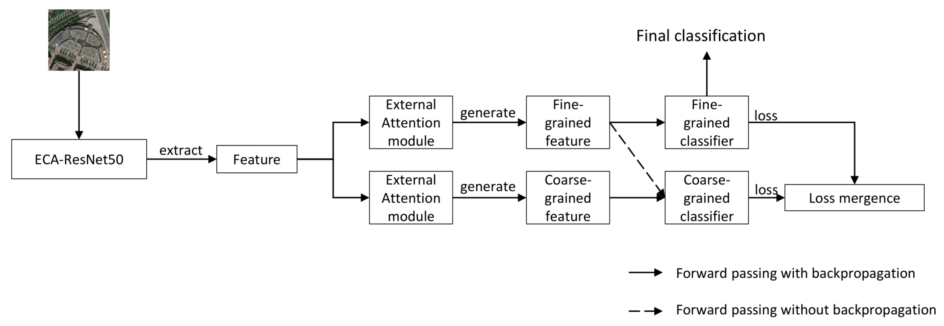
2.1. Multi-Task Multi-Grained Network
2.2. Gradient Control Module
2.3. Efficient Channel Attention Module
2.4. External Attention Module
3. Results
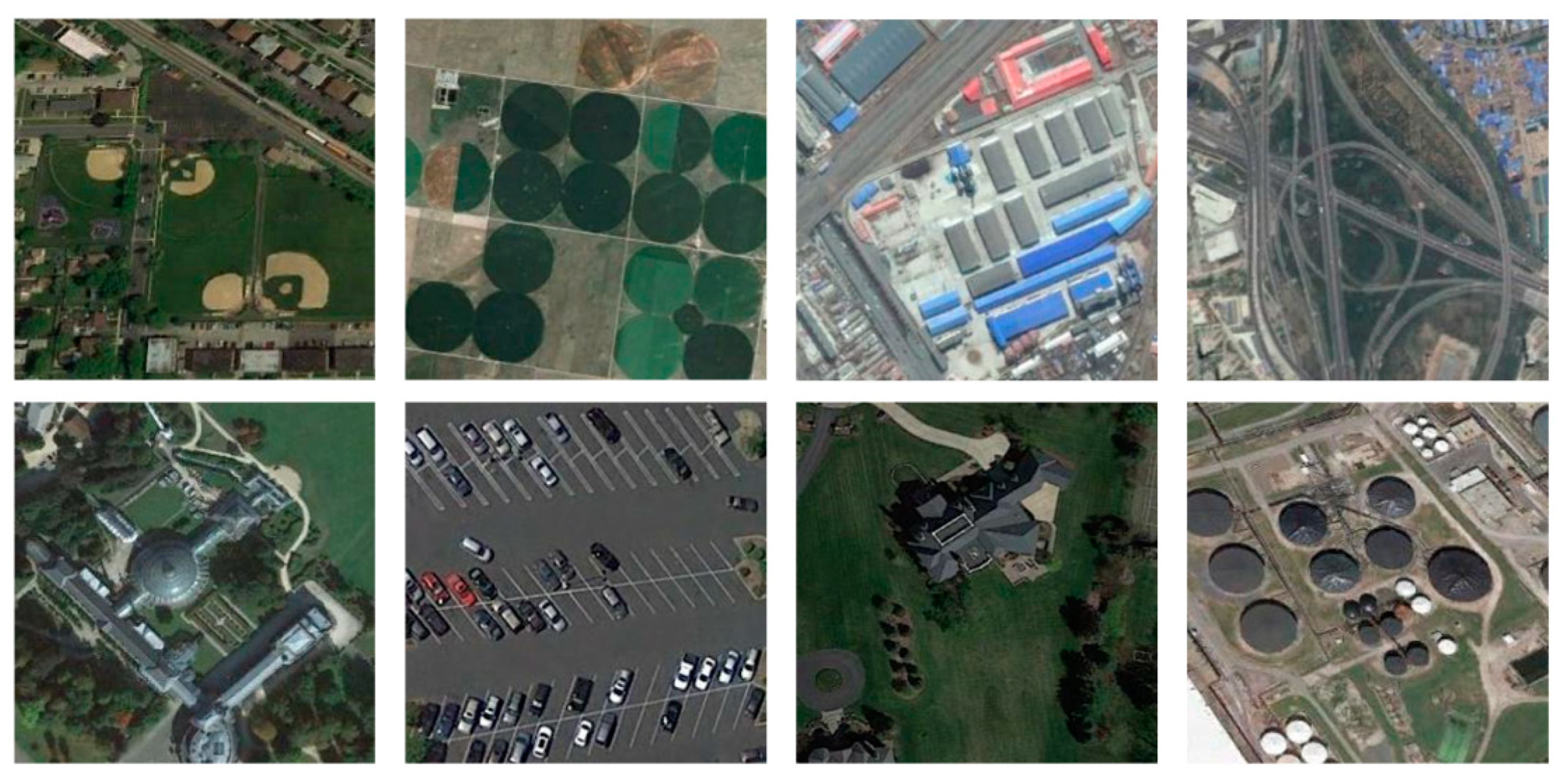
3.1. Dataset
3.2. Experimental Setup
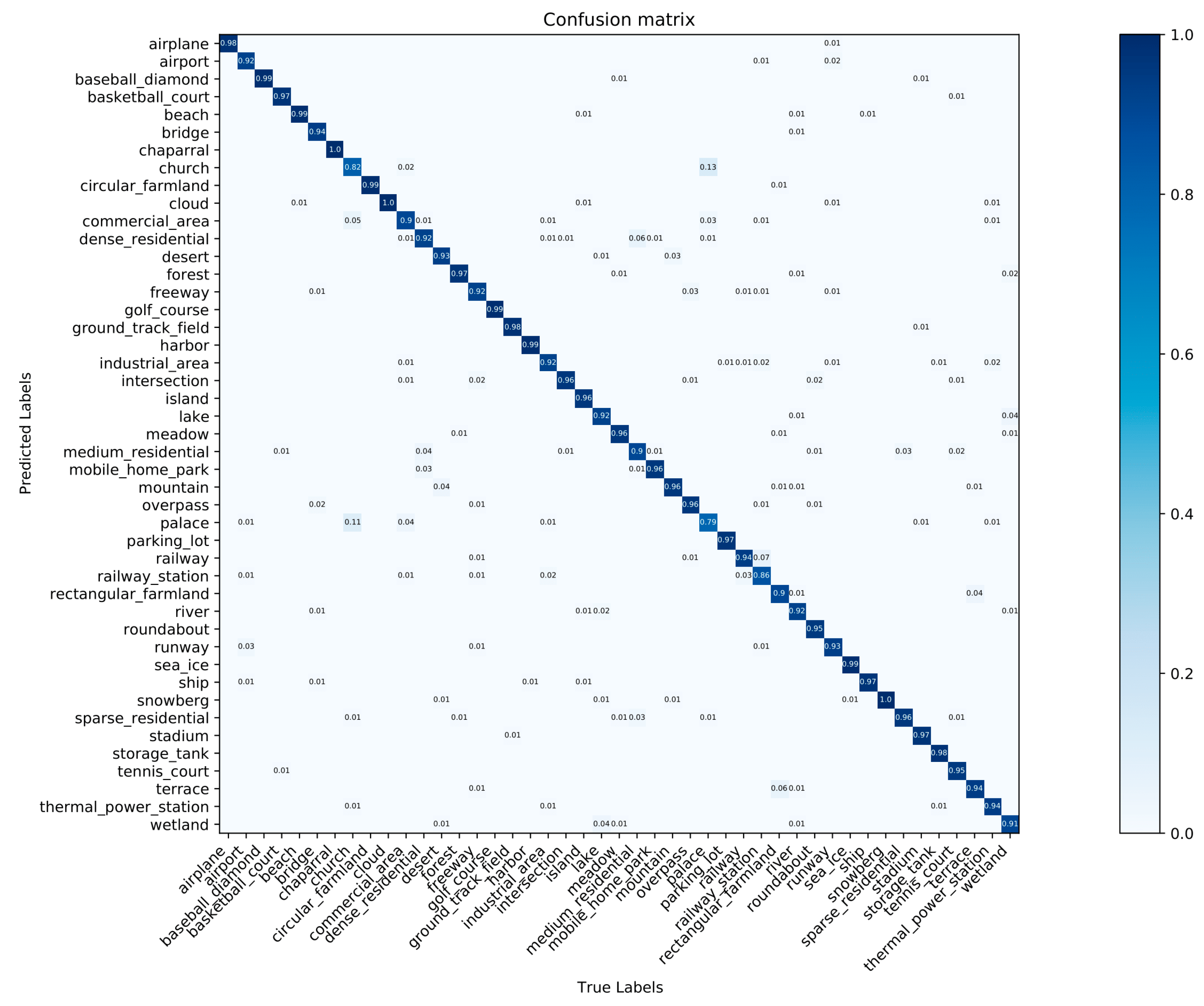
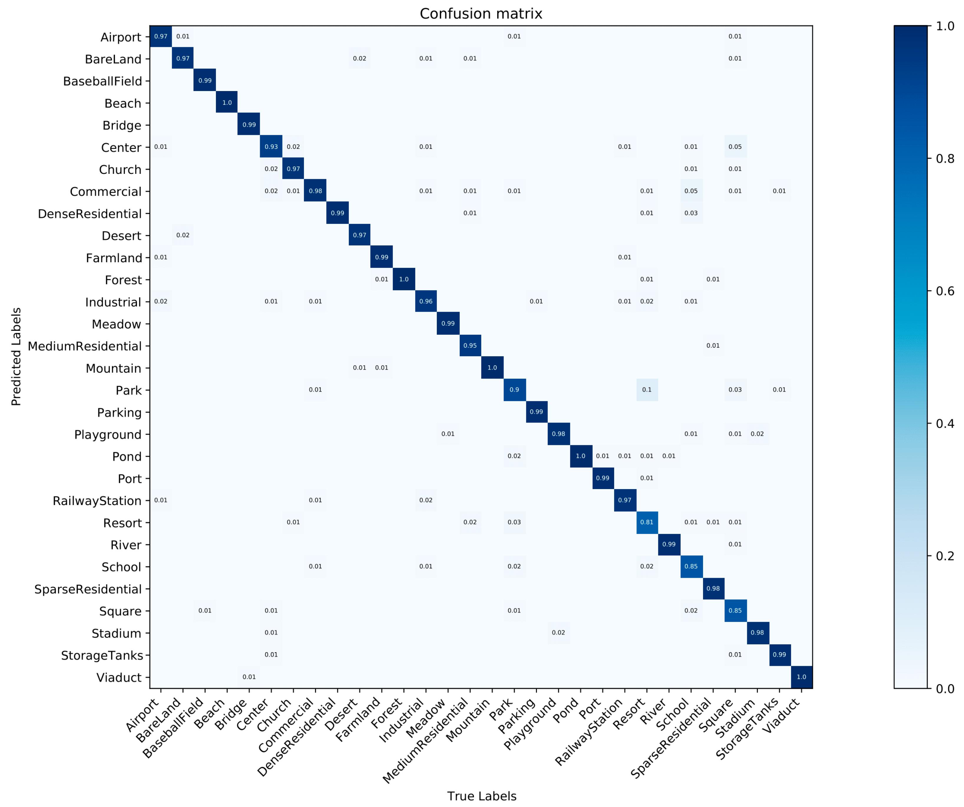
3.3. Experimental Results
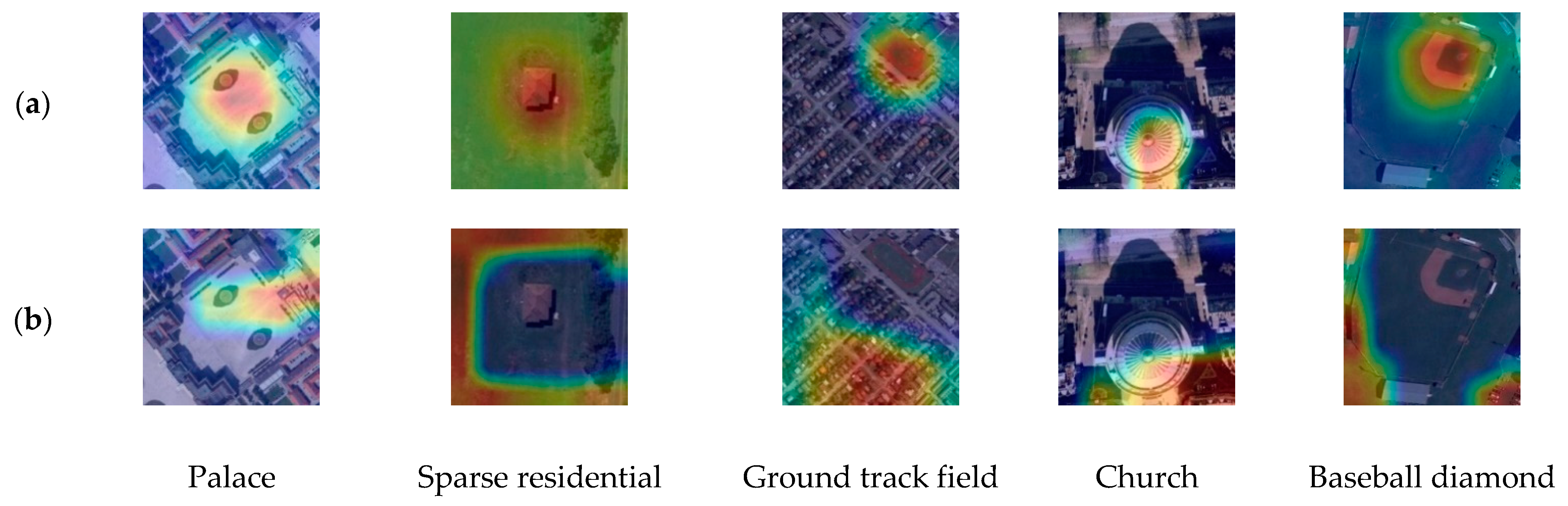
3.4. Discussion
3.5. Computational Complexity
4. Conclusions
Author Contributions
Funding
Institutional Review Board Statement
Informed Consent Statement
Data Availability Statement
Acknowledgments
Conflicts of Interest
References
- Sun, H.; Li, S.; Zheng, X.; Lu, X. Remote Sensing Scene Classification by Gated Bidirectional Network. IEEE Trans. Geosci. Remote Sens. 2020, 58, 82–96. [Google Scholar] [CrossRef]
- Zhang, L.; Zhang, L. Artificial Intelligence for Remote Sensing Data Analysis: A Review of Challenges and Opportunities. IEEE Geosci. Remote Sens. Mag. 2022, 10, 270–294. [Google Scholar] [CrossRef]
- Shen, H.; Jiang, M.; Li, J.; Zhou, C.; Yuan, Q.; Zhang, L. Coupling Model- and Data-Driven Methods for Remote Sensing Image Restoration and Fusion: Improving Physical Interpretability. IEEE Geosci. Remote Sens. Mag. 2022, 10, 231–249. [Google Scholar] [CrossRef]
- Chen, W.; Zheng, X.; Lu, X. Semisupervised Spectral Degradation Constrained Network for Spectral Super-Resolution. IEEE Geosci. Remote Sens. Lett. 2022, 19, 1–5. [Google Scholar] [CrossRef]
- Zheng, X.; Sun, H.; Lu, X.; Xie, W. Rotation-Invariant Attention Network for Hyperspectral Image Classification. IEEE Trans. Image Process. 2022, 31, 4251–4265. [Google Scholar] [CrossRef] [PubMed]
- Phung, M.T.; Tu, T.H. Scene Classification for Weak Devices Using Spatial Oriented Gradient Indexing. In Eighth International Conference on Graphic and Image Processing (ICGIP 2016); SPIE: Bellingham, WA, USA, 2017; Volume 10225, p. 1022520. [Google Scholar]
- Anwer, R.M.; Khan, F.S.; van de Weijer, J.; Molinier, M.; Laaksonen, J. Binary Patterns Encoded Convolutional Neural Networks for Texture Recognition and Remote Sensing Scene Classification. ISPRS J. Photogramm. Remote Sens. 2018, 138, 74–85. [Google Scholar] [CrossRef]
- Xia, G.S.; Hu, J.; Hu, F.; Shi, B.; Bai, X.; Zhong, Y.; Zhang, L.; Lu, X. AID: A Benchmark Data Set for Performance Evaluation of Aerial Scene Classification. IEEE Trans. Geosci. Remote Sens. 2017, 55, 3965–3981. [Google Scholar] [CrossRef]
- Li, F. Automatic Acquisition of Appropriate Codewords Number in BoVW Model and the Corresponding Scene Classification Performance. In Proceedings of the 37th Chinese Control Conference, Wuhan, China, 25–27 July 2018. [Google Scholar]
- Jegou, H.; Douze, M.; Schmid, C.; Perez, P. Aggregating Local Descriptors into a Compact Image Representation. In 2010 IEEE Computer Society Conference on Computer Vision and Pattern Recognition; IEEE: San Francisco, CA, USA, 2010; pp. 3304–3311. [Google Scholar]
- Perronin, F.; Larlus, D. Fisher Vectors Meet Neural Networks: A Hybrid Classification Architecture. In Proceedings of the 2015 IEEE Conference on Computer Vision and Pattern Recognition (CVPR), Boston, MA, USA, 7–12 June 2015. [Google Scholar]
- Lu, X.; Sun, H.; Zheng, X. A Feature Aggregation Convolutional Neural Network for Remote Sensing Scene Classification. IEEE Trans. Geosci. Remote Sens. 2019, 57, 7894–7906. [Google Scholar] [CrossRef]
- LeCun, Y.; Bottou, L.; Bengio, Y.; Haffner, P. Gradient-Based Learning Applied to Document Recognition. Proc. IEEE 1998, 86, 2278–2323. [Google Scholar] [CrossRef]
- Kipf, T.N.; Welling, M. Semi-Supervised Classification with Graph Convolutional Networks. In Proceedings of the International Conference on Learning Representations, Copenhagen, Denmark, 9–11 September 2017. [Google Scholar]
- Goodfellow, I.J.; Pouget-Abadie, J.; Mirza, M.; Xu, B.; Warde-Farley, D.; Ozair, S.; Courville, A.; Bengio, Y. Generative Adversarial Networks. arXiv 2014, arXiv:1406.2661. [Google Scholar] [CrossRef]
- He, K.; Zhang, X.; Ren, S.; Sun, J. Deep Residual Learning for Image Recognition. In Proceedings of the IEEE Computer Society Conference on Computer Vision and Pattern Recognition, Las Vegas, NV, USA, 27–30 June 2016; pp. 770–778. [Google Scholar]
- Zhang, X.; Zhou, X.; Lin, M.; Sun, J. ShuffleNet: An Extremely Efficient Convolutional Neural Network for Mobile Devices. In Proceedings of the IEEE Computer Society Conference on Computer Vision and Pattern Recognition, Salt Lake City, UT, USA, 18–23 June 2018; pp. 6848–6856. [Google Scholar]
- Tan, M.; Le, Q.V. EfficientNet: Rethinking Model Scaling for Convolutional Neural Networks. In Proceedings of the 36th International Conference on Machine Learning, Long Beach, CA, USA, 28 May 2019. [Google Scholar]
- Wang, B.; Dong, G.; Zhao, Y.; Li, R.; Cao, Q.; Chao, Y. Non-Uniform Attention Network for Multi-Modal Sentiment Analysis. In International Conference on Multimedia Modeling; Springer: Cham, Switzerland, 2022; pp. 612–623. [Google Scholar]
- Hao, S.; Zhang, H. Performance Analysis of PHY Layer for RIS-Assisted Wireless Communication Systems with Retransmission Protocols. J. King Saud Univ. Comput. Inf. Sci. 2022, 34, 5388–5404. [Google Scholar] [CrossRef]
- Li, F.; Feng, R.; Han, W.; Wang, L. High-Resolution Remote Sensing Image Scene Classification via Key Filter Bank Based on Convolutional Neural Network. IEEE Trans. Geosci. Remote Sens. 2020, 58, 8077–8092. [Google Scholar] [CrossRef]
- Wang, Q.; Huang, W.; Xiong, Z.; Li, X. Looking Closer at the Scene: Multiscale Representation Learning for Remote Sensing Image Scene Classification. IEEE Trans. Neural Netw. Learn. Syst. 2022, 33, 1414–1428. [Google Scholar] [CrossRef] [PubMed]
- Sun, H.; Zheng, X.; Lu, X. A Supervised Segmentation Network for Hyperspectral Image Classification. IEEE Trans. Image Process. 2021, 30, 2810–2825. [Google Scholar] [CrossRef] [PubMed]
- Xue, W.; Dai, X.; Liu, L. Remote Sensing Scene Classification Based on Multi-Structure Deep Features Fusion. IEEE Access 2020, 8, 28746–28755. [Google Scholar] [CrossRef]
- Castelluccio, M.; Poggi, G.; Sansone, C.; Verdoliva, L. Land Use Classification in Remote Sensing Images by Convolutional Neural Networks. arXiv 2015, arXiv:1508.00092. [Google Scholar]
- Tian, T.; Li, L.; Chen, W.; Zhou, H. SEMSDNet: A Multiscale Dense Network with Attention for Remote Sensing Scene Classification. IEEE J. Sel. Top. Appl. Earth Obs. Remote Sens. 2021, 14, 5501–5514. [Google Scholar] [CrossRef]
- Wang, Q.; Liu, S.; Chanussot, J.; Li, X. Scene Classification with Recurrent Attention of VHR Remote Sensing Images. IEEE Trans. Geosci. Remote Sens. 2019, 57, 1155–1167. [Google Scholar] [CrossRef]
- Chen, G.; Zhang, X.; Tan, X.; Cheng, Y.; Dai, F.; Zhu, K.; Gong, Y.; Wang, Q. Training Small Networks for Scene Classification of Remote Sensing Images via Knowledge Distillation. Remote Sens. 2018, 10, 719. [Google Scholar] [CrossRef]
- Zhang, B.; Zhang, Y.; Wang, S. A Lightweight and Discriminative Model for Remote Sensing Scene Classification with Multidilation Pooling Module. IEEE J. Sel. Top. Appl. Earth Obs. Remote Sens. 2019, 12, 2636–2653. [Google Scholar] [CrossRef]
- Ruder, S. An Overview of Multi-Task Learning in Deep Neural Networks. arXiv 2017, arXiv:1706.05098. [Google Scholar]
- Chang, D.; Pang, K.; Zheng, Y.; Ma, Z.; Song, Y.Z.; Guo, J. Your “Flamingo” Is My “Bird”: Fine-Grained, or Not. In Proceedings of the IEEE Computer Society Conference on Computer Vision and Pattern Recognition, Nashville, TN, USA, 20–25 June 2021; pp. 11471–11480. [Google Scholar]
- Liu, P.; Qiu, X.; Huang, X. Recurrent Neural Network for Text Classification with Multi-Task Learning. arXiv 2016, arXiv:1605.05101. [Google Scholar] [CrossRef]
- Crawshaw, M. Multi-Task Learning with Deep Neural Networks: A Survey. arXiv 2020, arXiv:2009.09796. [Google Scholar]
- Wang, Q.; Wu, B.; Zhu, P.; Li, P.; Zuo, W.; Hu, Q. ECA-Net: Efficient Channel Attention for Deep Convolutional Neural Networks. In Proceedings of the IEEE Computer Society Conference on Computer Vision and Pattern Recognition, Seattle, WA, USA, 14–19 June 2020; pp. 11531–11539. [Google Scholar]
- Kokkinos, I. UberNet: Training a ‘Universal’ Convolutional Neural Network for Low-, Mid-, and High-Level Vision Using Diverse Datasets and Limited Memory. In Proceedings of the 2017 IEEE Conference on Computer Vision and Pattern Recognition (CVPR), Honolulu, HI, USA, 21–26 July 2017. [Google Scholar]
- Zhang, W.; Tang, P.; Zhao, L. Remote Sensing Image Scene Classification Using CNN-CapsNet. Remote Sens. 2019, 11, 494. [Google Scholar] [CrossRef]
- Cheng, G.; Han, J.; Lu, X. Remote Sensing Image Scene Classification: Benchmark and State of the Art. Proc. IEEE 2017, 105, 1865–1883. [Google Scholar] [CrossRef]
- Loshchilov, I.; Hutter, F. SGDR: Stochastic Gradient Descent with Warm Restarts. In Proceedings of the 5th International Conference on Learning Representations, San Juan, Puerto Rico, 2–4 May 2016. [Google Scholar] [CrossRef]
- Szegedy, C.; Liu, W.; Jia, Y.; Sermanet, P.; Reed, S.; Anguelov, D.; Erhan, D.; Vanhoucke, V.; Rabinovich, A. Going Deeper with Convolutions. In Proceedings of the IEEE Computer Society Conference on Computer Vision and Pattern Recognition, Boston, MA, USA, 7–12 June 2015; pp. 1–9. [Google Scholar]
- Simonyan, K.; Zisserman, A. Very Deep Convolutional Networks for Large-Scale Image Recognition. In Proceedings of the International Conference on Learning Representations, San Diego, CA, USA, 7–9 May 2015; pp. 1–14. [Google Scholar]
- Cheng, G.; Yang, C.; Yao, X.; Guo, L.; Han, J. When Deep Learning Meets Metric Learning: Remote Sensing Image Scene Classification via Learning Discriminative CNNs. IEEE Trans. Geosci. Remote Sens. 2018, 56, 2811–2821. [Google Scholar] [CrossRef]
- Wang, S.; Guan, Y.; Shao, L. Multi-Granularity Canonical Appearance Pooling for Remote Sensing Scene Classification. IEEE Trans. Image Process. 2020, 29, 5396–5407. [Google Scholar] [CrossRef]
- Shi, C.; Zhang, X.; Sun, J.; Wang, L. Remote Sensing Scene Image Classification Based on Dense Fusion of Multi-Level Features. Remote Sens. 2021, 13, 4379. [Google Scholar] [CrossRef]
- He, N.; Fang, L.; Li, S.; Plaza, J.; Plaza, A. Skip-Connected Covariance Network for Remote Sensing Scene Classification. IEEE Trans. Neural Netw. Learn. Syst. 2020, 31, 1461–1474. [Google Scholar] [CrossRef]
- Wang, X.; Duan, L.; Shi, A.; Zhou, H. Multilevel Feature Fusion Networks with Adaptive Channel Dimensionality Reduction for Remote Sensing Scene Classification. IEEE Geosci. Remote Sens. Lett. 2022, 19, 1–5. [Google Scholar] [CrossRef]
- Wang, W.; Chen, Y.; Ghamisi, P. Transferring CNN with Adaptive Learning for Remote Sensing Scene Classification. IEEE Trans. Geosci. Remote Sens. 2022, 60, 1–18. [Google Scholar] [CrossRef]
- Shen, J.; Yu, T.; Yang, H.; Wang, R.; Wang, Q. An Attention Cascade Global–Local Network for Remote Sensing Scene Classification. Remote Sens. 2022, 14, 2042. [Google Scholar] [CrossRef]
- Ciampi, L.; Messina, N.; Falchi, F.; Gennaro, C.; Amato, G. Virtual to Real Adaptation of Pedestrian Detectors. Sensors 2020, 20, 5250. [Google Scholar] [CrossRef] [PubMed]
- Staniszewski, M.; Foszner, P.; Kostorz, K.; Michalczuk, A.; Wereszczyński, K.; Cogiel, M.; Golba, D.; Wojciechowski, K.; Polański, A. Application of Crowd Simulations in the Evaluation of Tracking Algorithms. Sensors 2020, 20, 4960. [Google Scholar] [CrossRef] [PubMed]


| Coarse-Grained Label | Fine-Grained Label |
|---|---|
| Cultivated | Circular farmland |
| Rectangular farmland | |
| Terrace | |
| Woodland | Chaparral |
| Forest | |
| Wetland | |
| Grassland | Meadow |
| Commercial Service | Commercial area |
| Industrial and Mining | Industrial area |
| Thermal power station | |
| Residential | Dense residential |
| Medium residential | |
| Sparse residential | |
| Public | Baseball diamond |
| Basketball court | |
| Golf course | |
| Ground track field | |
| Mobile home park | |
| Runway | |
| Tennis court | |
| Stadium | |
| Special | Church |
| Palace | |
| Storage tanks | |
| Transportation land | Airport |
| Airplane | |
| Bridge | |
| Freeway | |
| Harbor | |
| Intersection | |
| Overpass | |
| Parking lot | |
| railway | |
| Railway station | |
| Roundabout | |
| Water | Beach |
| Island | |
| Lake | |
| River | |
| Sea ice | |
| Ship | |
| Iceberg | |
| Other | Cloud |
| Desert | |
| Mountain |
| Coarse-Grained Label | Fine-Grained Label |
|---|---|
| Cultivated | Farmland |
| Woodland | Forest |
| Grassland | Meadow |
| Commercial Service | Commercial |
| Industrial and Mining | Industrial |
| Residential | Dense residential |
| Medium residential | |
| Sparse residential | |
| Public | Baseball Field |
| Center | |
| Park | |
| Playground | |
| School | |
| Square | |
| Stadium | |
| Special | Church |
| Resort | |
| Storage tanks | |
| Transportation land | Airport |
| Bridge | |
| Parking | |
| Port | |
| Railway station | |
| Viaduct | |
| Water | Beach |
| Pond | |
| River | |
| Other | Bare land |
| Desert | |
| Mountain |
| Methods | Overall Accuracy | |
|---|---|---|
| 10% Training Ratio | 20% Training Ratio | |
| (Fine-tuning) GoogleNet [39] | 82.57 ± 0.14 | 86.02 ± 0.18 |
| (Fine-tuning) VGG-16 [40] | 87.15 ± 0.45 | 90.36 ± 0.18 |
| (Fine-tuning) ResNet50 [16] | 88.48 ± 0.21 | 91.86 ± 0.19 |
| D-CNN [41] | 89.22 ± 0.50 | 91.89 ± 0.22 |
| MG-CAP [42] | 90.83 ± 0.12 | 92.85 ± 0.11 |
| BMDF-LCNN [43] | 91.65 ± 0.15 | 93.5 ± 70.22 |
| SCCov [44] | 89.30 ± 0.35 | 92.10 ± 0.25 |
| MLFF [45] | 90.01 ± 0.33 | 92.45 ± 0.20 |
| T-CNN [46] | 90.25 ± 0.14 | 93.05 ± 0.12 |
| Ours | 92.07 ± 0.14 | 94.53 ± 0.11 |
| Methods | Overall Accuracy | |
|---|---|---|
| 10% Training Ratio | 20% Training Ratio | |
| (Fine-tuning) GoogleNet [39] | 83.44 ± 0.40 | 86.39 ± 0.55 |
| (Fine-tuning) VGG-16 [40] | 86.59 ± 0.29 | 89.64 ± 0.36 |
| (Fine-tuning) ResNet50 [16] | 92.57 ± 0.21 | 95.96 ± 0.17 |
| D-CNN [41] | 90.82 ± 0.16 | 96.89 ± 0.10 |
| MG-CAP [42] | 93.34 ± 0.18 | 96.12 ± 0.12 |
| ACGLNet [47] | 94.44 ± 0.09 | 96.10 ± 0.10 |
| BMDF-LCNN [43] | 94.46 ± 0.15 | 96.76 ± 0.18 |
| SCCov [44] | 93.12 ± 0.25 | 96.89 ± 0.10 |
| MLFF [45] | 92.73 ± 0.12 | 95.06 ± 0.33 |
| T-CNN [46] | 94.55 ± 0.27 | 96.72 ± 0.23 |
| Ours | 94.96 ± 0.13 | 96.72 ± 0.12 |
Publisher’s Note: MDPI stays neutral with regard to jurisdictional claims in published maps and institutional affiliations. |
© 2022 by the authors. Licensee MDPI, Basel, Switzerland. This article is an open access article distributed under the terms and conditions of the Creative Commons Attribution (CC BY) license (https://creativecommons.org/licenses/by/4.0/).
Share and Cite
Zeng, P.; Lin, S.; Sun, H.; Zhou, D. Exploiting Hierarchical Label Information in an Attention-Embedding, Multi-Task, Multi-Grained, Network for Scene Classification of Remote Sensing Imagery. Appl. Sci. 2022, 12, 8705. https://doi.org/10.3390/app12178705
Zeng P, Lin S, Sun H, Zhou D. Exploiting Hierarchical Label Information in an Attention-Embedding, Multi-Task, Multi-Grained, Network for Scene Classification of Remote Sensing Imagery. Applied Sciences. 2022; 12(17):8705. https://doi.org/10.3390/app12178705
Chicago/Turabian StyleZeng, Peng, Shixuan Lin, Hao Sun, and Dongbo Zhou. 2022. "Exploiting Hierarchical Label Information in an Attention-Embedding, Multi-Task, Multi-Grained, Network for Scene Classification of Remote Sensing Imagery" Applied Sciences 12, no. 17: 8705. https://doi.org/10.3390/app12178705
APA StyleZeng, P., Lin, S., Sun, H., & Zhou, D. (2022). Exploiting Hierarchical Label Information in an Attention-Embedding, Multi-Task, Multi-Grained, Network for Scene Classification of Remote Sensing Imagery. Applied Sciences, 12(17), 8705. https://doi.org/10.3390/app12178705