Bridge Modal Parameter Identification from UAV Measurement Based on Empirical Mode Decomposition and Fourier Transform

Abstract

This paper proposes two approaches, Empirical Mode Decomposition (EMD) and Fourier Transform (FT), to correct the vibration signals measured by an Unmanned Aerial Vehicle (UAV), which overcomes the difficulty of selection of reference points used in other correction methods, such as homography transformation and three-dimensional reconstruction. In the method of this paper, a UAV is used to collect the video of a vibrated bridge, and the displacement signal of the bridge is obtained from the video by Kanade–Lucas–Tomasi (KLT) optical flow method, which contains false displacement caused by the ego-motion of the UAV during the measurement. The false displacement can be effectively eliminated by EMD and FT to obtain the real displacement signal. Finally, the displacement signal is processed by the Operational Modal Analysis (OMA) technique to obtain the bridge modal parameters. The performance of correcting vibration signals and extracting bridge modal parameters from the vibration signals based on EMD, FT, and Differential Filtering (DF) are compared by taking the fixed camera measurement as a reference (the accuracy of measuring bridge vibration with fixed cameras has been verified) in this paper, and it is demonstrated that EMD has better reliability in processing signal measured by UAVs, which is mainly due to the absence of random factors and too much noise in the signal processing process of EMD.

1. Introduction

Damage detection of bridge structures is an essential procedure in the long-term service of bridges, and measuring vibration is indispensable in the process of damage identification [1]. Strain gauges [2] and acceleration sensors [3] are the traditional methods to measure vibration of bridge structure, but due to the disadvantages of contact measurement, non-contact measurement methods such as Laser Doppler Vibrometer (LDV) [4] and Global Positioning System (GPS) [5] are gradually getting popular. With the development of measurement technology, GPS and LDV are gradually replaced by some optical measurement methods with higher precision and lower cost. Kanade–Lucas–Tomasi (KLT) optical flow method [6] is a measurement method of computer vision, which is an improved method of Lucas–Kanade (LK) optical flow method [7]. The inter-frame motion information of target points is obtained by tracking the target points on a set of images stored in frames by KLT. As KLT performs well in target tracking [8], it has been applied to vibration measurement of bridge models [9]. Fixed cameras are normally used in optical measurement methods. However, it is difficult to select appropriate installation locations for fixed cameras under some conditions (such as cross-valley bridges). With their wide applications, Unmanned Aerial Vehicles (UAVs) [10,11,12] have become popular in bridge measurement [13,14].

Due to the motion of UAVs during the measurement, false displacement is introduced in the measured displacement results [15]. Homography transformation [16] is a commonly used method to correct the displacement measured by UAVs. Four fixed reference points are used to calculate the homography matrix between the reference frame and other frames in this method, and the displacement of the target point on the bridge can be corrected by the homography transformation. However, this method requires the target points on the bridge and four fixed reference points to be in the same plane, and that is unrealistic in actual bridge measurement. The world coordinates of the target points on the bridge can be recovered by the three-dimensional reconstruction, and the displacement time–history curves of the target points can be obtained [17]. But the plane of target points and that of reference points are required to be parallel for this method, and the distance between two planes also needs to be known in advance, which is difficult to satisfy in the process of actual bridge measurement. As neural networks are developed, they are gradually applied to solve the problem of unstable shooting of UAVs. The characteristic relationship between the target points on the measured bridge and the reference points on the background can be learned by a Feedforward Neural Network (FNN), and true displacement of the target points can be predicted through the characteristic relationship by the trained FNN [18]. Although the false displacement caused by UAVs can be eliminated by this method, some fixed reference points on the background of the bridge are also required for this method, and that is difficult to realize in some cases (e.g., the background of the bridge is the boundless sea).

The modal parameters of bridges can be obtained from the vibration signals measured by UAVs based on the Differential Filtering (DF) technique [19] without using any reference points [20]. In this method, the acceleration signal of the bridge can be obtained from original signal measured by UAVs by second-order differential filtering. However, the random signal caused by the UAV motion cannot be effectively eliminated by this method, which leads to the low accuracy of the obtained bridge modal parameters. According to the original signal characteristics in the time scale, finite Intrinsic Mode Functions (IMF) can be obtained by decomposing complex signals through Empirical Mode Decomposition (EMD) [21,22], and each IMF contains different local characteristics in the time scale. EMD perform well in processing non-stationary and nonlinear data for its universality, and it is widely used in processing displacement signal [23]. The time-domain signal can be converted into frequency-domain signal, that is, the spectrum of signal, by Fourier Transform (FT) [24]. It is believed that any continuously measured time signal can be expressed by the FT as infinite superposition of sine wave signals with different frequencies. The FT is widely used in the field of signals processing [25]. The original time domain signals can be obtained from the frequency domain signals by Inverse Fourier Transform (IFT) [26]. The EMD and the FT (combined with IFT) can be used respectively to process the displacement signal of the bridge measured by a UAV, and the bridge modal parameters are extracted from the processed signals through Operational Modal Analysis (OMA) [27,28]. In OMA process, the structural natural frequency can be identified by Power Spectral Density (PSD) [29], while the ratio of the PSD Transmissibility (PSDT) [30] is used to obtain the bridge mode shape [31].

In this paper, EMD and FT are used to eliminate the random component in the signals of a bridge model measured by a UAV. The bridge vibration is video-recorded by a UAV, the target points on the bridge model in the video are tracked by KLT, and their displacement contains false component. Then the EMD and FT are used to process displacement signals, respectively. The modal parameters of the bridge model can be obtained by analyzing the processed signals with OMA. Finally, taking the fixed camera measurement as a reference, the processing effects and the modal parameter identification accuracies of EMD, FT, and DF are compared.

2. Methods

2.1. KLT Optical-Flow Method

The unchanged pixel value of each point and the small motion of each point between adjacent frames are presumed in the KLT. In addition, spatial consistency is another assumption of this method, that is, the adjacent pixels have similar motion between adjacent frames. The image pyramid technique [32] is used by KLT to meet the assumption of spatial consistency under different conditions.

The target points selected in the first frame are used to calculate the inter-frame vector to realize target tracking by KLT. Suppose $W$ is a constant size window, which is centered on the position of a target point on each frame image and $d_x$ and $d_y$ are the motion of the target point along the x-axis and y-axis between 2 frames; the motion, $\mathit{d}={\left[\begin{array}{cc}{d}_x& d_y\end{array}\right]}^T$, can be obtained by minimizing the value of the following formula [6]:

$$\begin{array}{c}\epsilon ={{\displaystyle \iint }}_W^{}{\left[I_2\left(\mathit{X}+\mathit{d}\right)-I_1\left(\mathit{X}\right)\right]}^2\omega \left(\mathit{X}\right)d\mathit{X}\end{array}$$

(1)

where $\epsilon$ is the residual error, $I_1$ is the image of the previous frame, $I_2$ is the image of the next frame, $\omega \left(\mathit{X}\right)$ is the weight function, $\mathit{X}={\left[\begin{array}{cc}x& y\end{array}\right]}^T$, $\left(x,y\right)$ are the coordinates of the pixels in the window, $W$.

From the video taken by the UAV, the coordinate of the target points on each frame can be obtained by KLT. The target points displacement time–history curves are obtained by connecting the coordinate information of each frame.

2.2. Correction Technique of Displacement Signal Measured by UAV

It can be seen from the previous section that the displacement time–history curve of the bridge can be obtained by tracking the target points in the video taken by the UAV through KLT, but the displacement signals contain the false displacement. Three techniques of eliminating the random signal caused by the UAV will be introduced in this section, including the two techniques used in this paper and the existing differential filtering technique.

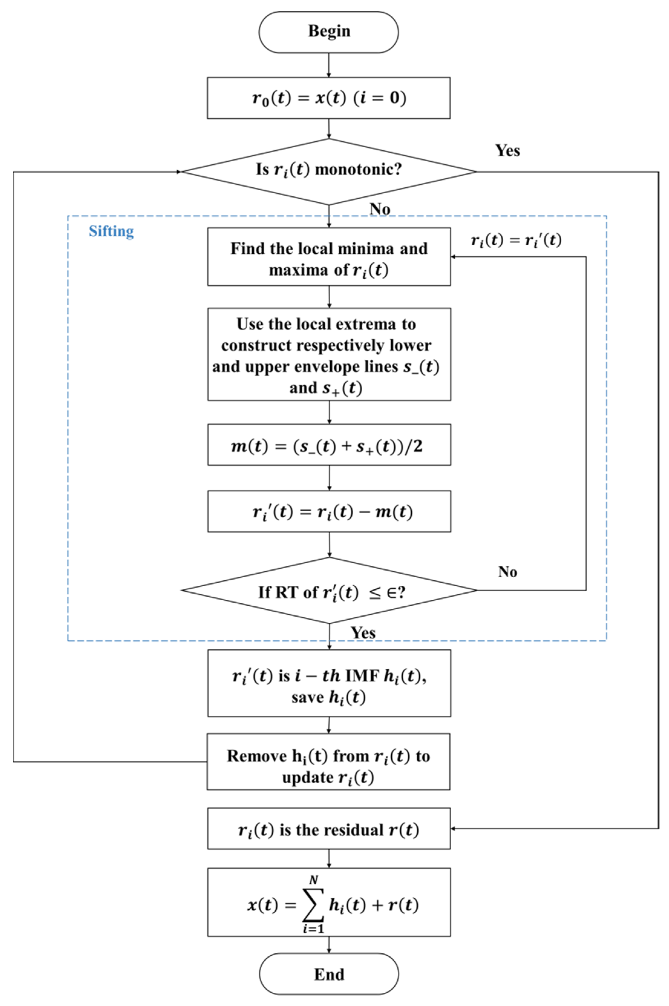
2.2.1. Empirical Mode Decomposition

A residual $r\left(t\right)$ and $N$ IMFs $h_i\left(t\right)$ can be obtained by decomposing the original signal $x\left(t\right)$ through an iterative sifting process by the EMD:

$$\begin{array}{c}x\left(t\right)={\displaystyle {\displaystyle \sum }_{i=1}^N}{h}_i\left(t\right)+r\left(t\right)\end{array}$$

(2)

where one of the $h_i\left(t\right)$ is the bridge true displacement signal, $N$ is the number of IMFs.

The process of EMD is shown in Figure 1. When the original signal $x\left(t\right)$ is not monotonic, it is put into the sifting process as $r_i\left(t\right) \left(i=0\right)$. The sifting process is as follows: the upper and lower envelope curves of the signal are formed by finding the local extremum of the signal, and the mean curves $m\left(t\right)$ of the upper envelope $s_{+}\left(t\right)$ and lower envelope $s_{-}\left(t\right)$ are removed from the signal to obtain a new signal ${r_i}^{\prime }\left(t\right)$. If ${r_i}^{\prime }\left(t\right)$ does not meet Equation (3), it will be put into the sifting process again, otherwise, ${r_i}^{\prime }\left(t\right)$ is the first IMF $h_i\left(t\right) \left(i=1\right)$, and the sifting process is ended. Remove the obtained first IMF from the original signal to obtain a new signal, and judge whether the new signal is monotonous. If not, repeat the above process; otherwise, it is the residual separated from the original signal, and the decomposition process is ended. The resulting residual and all IMFs are the components of the original data. The expression of RT of ${r_i}^{\prime }\left(t\right)$ is as follows:

$$\begin{array}{c}RT=\frac{{\displaystyle \sum }{\left[r_i^{\prime }\left(t\right)-r_i\left(t\right)\right]}^2}{{\displaystyle \sum }{\left[r_i\left(t\right)\right]}^2}\le \in \end{array}$$

(3)

where $\in$ can be set between 0.2 and 0.3 [21].

The signal measured by a UAV including false displacement can be decomposed with EMD to obtain the true vibration signal of the bridge, which is one of the IMFs. EMD is not only suitable for the analysis of nonlinear and non-stationary signals but also suitable for the analysis of linear and stationary signals.

2.2.2. Fourier Transform and Inverse Fourier Transform

The time domain signals can be converted into frequency domain signals with FT, which is a signal processing technique. For discrete data set $X$, the expression of FT is as follows [33]:

$$\begin{array}{c}{y}_{k+1}={\displaystyle {\displaystyle \sum }_{j=0}^{n-1}}{\omega }^{jk}{x}_{j+1}\end{array}$$

(4)

where $y_{k+1}$ is the new signal after FT, $x_{j+1}\in X$, $\omega =e^{\frac{-2\pi i}{n}}$ is one of the complex unit roots, $i$ is an imaginary unit, $n$ is the number of samples in $X$, and the value ranges of $j$ and $k$ are both 0 to $n-1$.

The frequency domain signals can be converted into time domain signals with IFT, and its expression is as follows:

$$\begin{array}{c}{x}_{j+1}=\frac{1}{n}{\displaystyle {\displaystyle \sum }_{k=0}^{n-1}}{\omega }^{-jk}{y}_{k+1}\end{array}$$

(5)

The FT used in this paper is generally used for continuous signal processing. The displacement signal measured by the UAV includes the bridge true displacement and the false displacement, and the vibration frequency of the UAV is small relative to the vibration frequency of the bridge; therefore, a filter combined FT with IFT is used to filter out the low-frequency signal. The spectrum diagram is obtained from the displacement signal with FT, and the low-frequency part of the spectrum is removed. Then the frequency domain signal is converted into the time domain signal with IFT, so as to obtain the bridge true vibration signal.

2.2.3. Differential Filtering

The noise and the zero drift of the signal measured by UAVs can be solved with DF, and the expression of DF is as follows:

$$\begin{array}{c}{y}_k=x_{k+2}+x_k-2x_{k+1}\end{array}$$

(6)

where $x_k$ is the k-th point of displacement signal, $y_k$ is the k-th point of acceleration signal obtained from the original signal by second-order differential filtering [34].

The DF is generally used for continuous signal processing. The vibration signal will be amplified by the square of the frequency by the differential filtering and that is conducive to the natural frequency identification [17].

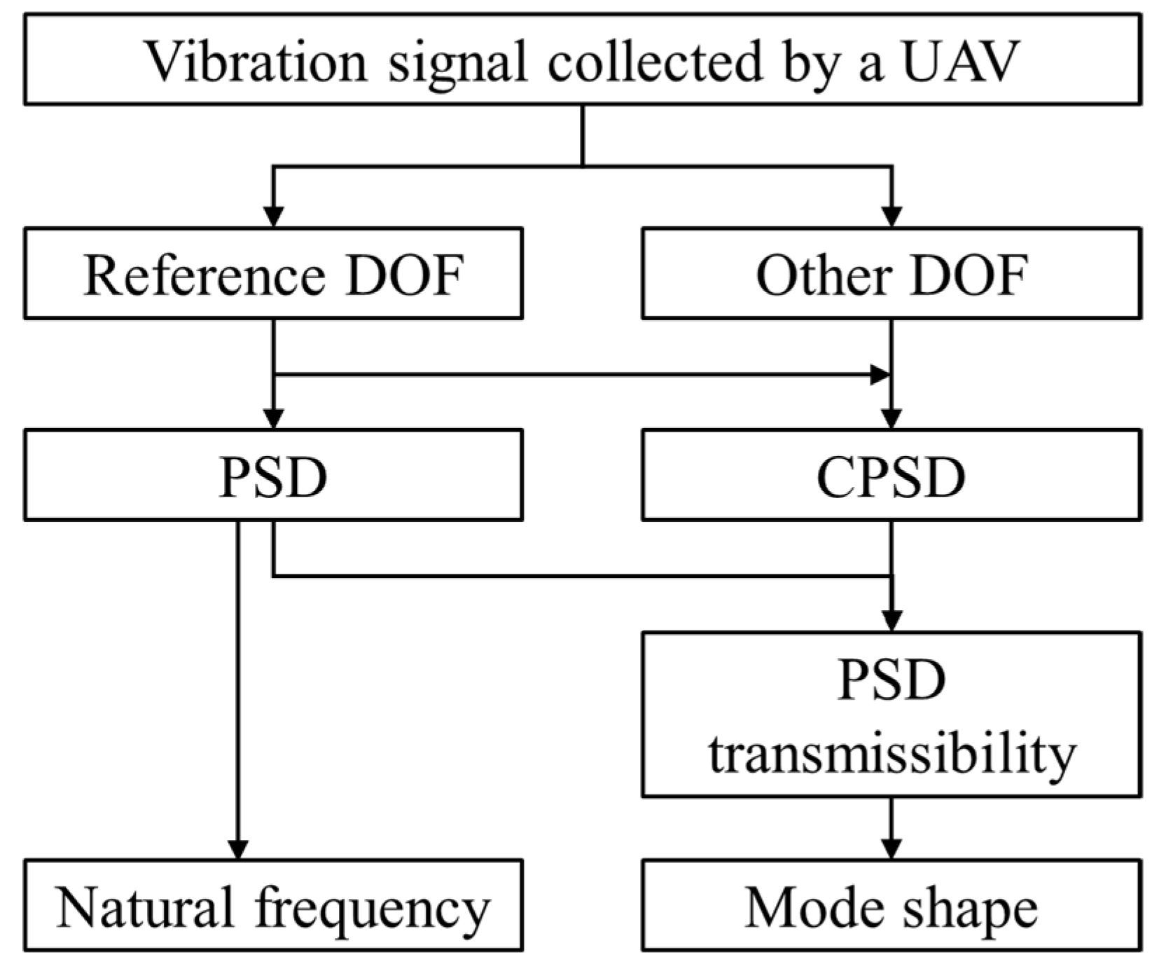
2.3. Operational Modal Analysis

In the process of OMA, the expression of response transmissibility in the multiple-degrees-of-freedom system is as follows [35]:

$$\begin{array}{c}{T}_{io}\left(\omega \right)=\frac{X_i\left(\omega \right)}{X_o\left(\omega \right)}\end{array}$$

(7)

where $T_{io}\left(\omega \right)$ is response transmissibility; $X_i\left(\omega \right)$ and $X_o\left(\omega \right)$ are the Fourier transforms of $x_i\left(t\right)$ and $x_o\left(t\right)$ at the Degrees of Freedom (DOF) $i$ and $o,$ respectively.

The expression of Power Spectrum Density (PSD) transmissibility is as follows:

$$\begin{array}{c}{\widehat{T}}_{io}\left(\omega \right)=\frac{S_{i,o}\left(\omega \right)}{S_{o,o}\left(\omega \right)}=\frac{X_i\left(\omega \right)X_o^{*}\left(\omega \right)}{X_o\left(\omega \right)X_o^{*}\left(\omega \right)}\end{array}$$

(8)

where $X_o^{*}\left(\omega \right)$ is the conjugate complex number of $X_o\left(\omega \right)$, $S_{i,o}\left(\omega \right)$ is the Cross Power Spectrum Density (CPSD) of $x_i\left(\omega \right)$ and $x_o\left(\omega \right)$; $S_{o,o}\left(\omega \right)$ is the PSD of $x_o\left(\omega \right)$. The PSD transmissibility can be expressed as [36]:

$$\begin{array}{c}{\widehat{T}}_{io}\left(\omega \right)=\frac{X_i\left(\omega \right)}{X_o\left(\omega \right)}=\frac{H_{ip}\left(\omega \right)\cdot F_p\left(\omega \right)}{H_{op}\left(\omega \right)\cdot F_p\left(\omega \right)}=\frac{H_{ip}\left(\omega \right)}{H_{op}\left(\omega \right)}=T_{io}\left(\omega \right)\end{array}$$

(9)

where $H_{ip}\left(\omega \right)$ is the Frequency Response Function (FRF) between the degrees of freedom $i$ and $p$ [37], $F_p\left(\omega \right)$ is the Fourier transform of excitation force signal at point P. From the Equation (7), we can get the following:

$$\begin{array}{c}\underset{\omega \to {\omega }_r}{lim}{\widehat{T}}_{io}\left(\omega \right)=\underset{\omega \to {\omega }_r}{lim}\frac{H_{ip}\left(\omega \right)}{H_{op}\left(\omega \right)}=\frac{{\phi }_{ri}}{{\phi }_{ro}}\end{array}$$

(10)

Take the node of degree of freedom $o$ as the reference point, and change the order of measurement points of degree of freedom $i$ in turn ($i=1,2,...,N$). The r-th modal shape of the structure can be expressed as

$$\begin{array}{c}\left[\begin{array}{c}{\phi }_{r1}\\ {\phi }_{r2}\\ ⋮\\ {\phi }_{rN}\end{array}\right]={\phi }_{ro}\left[\begin{array}{c}{\hat{T}}_{1o}\left({\omega }_r\right)\\ {\hat{T}}_{2o}\left({\omega }_r\right)\\ ⋮\\ {\hat{T}}_{No}\left({\omega }_r\right)\end{array}\right]\end{array}$$

(11)

The structural modal shape can be obtained from Equation (7):

$$\begin{array}{c}{\phi }_r=\underset{\omega \to {\omega }_r}{lim}\left\{{\hat{T}}_{1o}\left(\omega \right),{\hat{T}}_{2o}\left(\omega \right),\dots ,{\hat{T}}_{no}\left(\omega \right)\right\}\end{array}$$

(12)

Substituting Equation (7) into Equation (11):

$$\begin{array}{c}{\phi }_r=\underset{\omega \to {\omega }_r}{lim}\left\{S_{1,o}\left(\omega \right),S_{2,o}\left(\omega \right),\dots ,S_{n,o}\left(\omega \right)\right\}\end{array}$$

(13)

The modal parameter identification process of a structure by OMA is shown in Figure 2. The PSD curve can be obtained from vibration signal under the reference DOF, and the structural natural frequency is obtained from the PSD curve [38]. The CPSD can be obtained from vibration signal under the reference DOF and other DOF, and the PSD transmissibility can be obtained according to Equation (8). The mode shape can be obtained by the PSD transmissibility.

3. Experiment

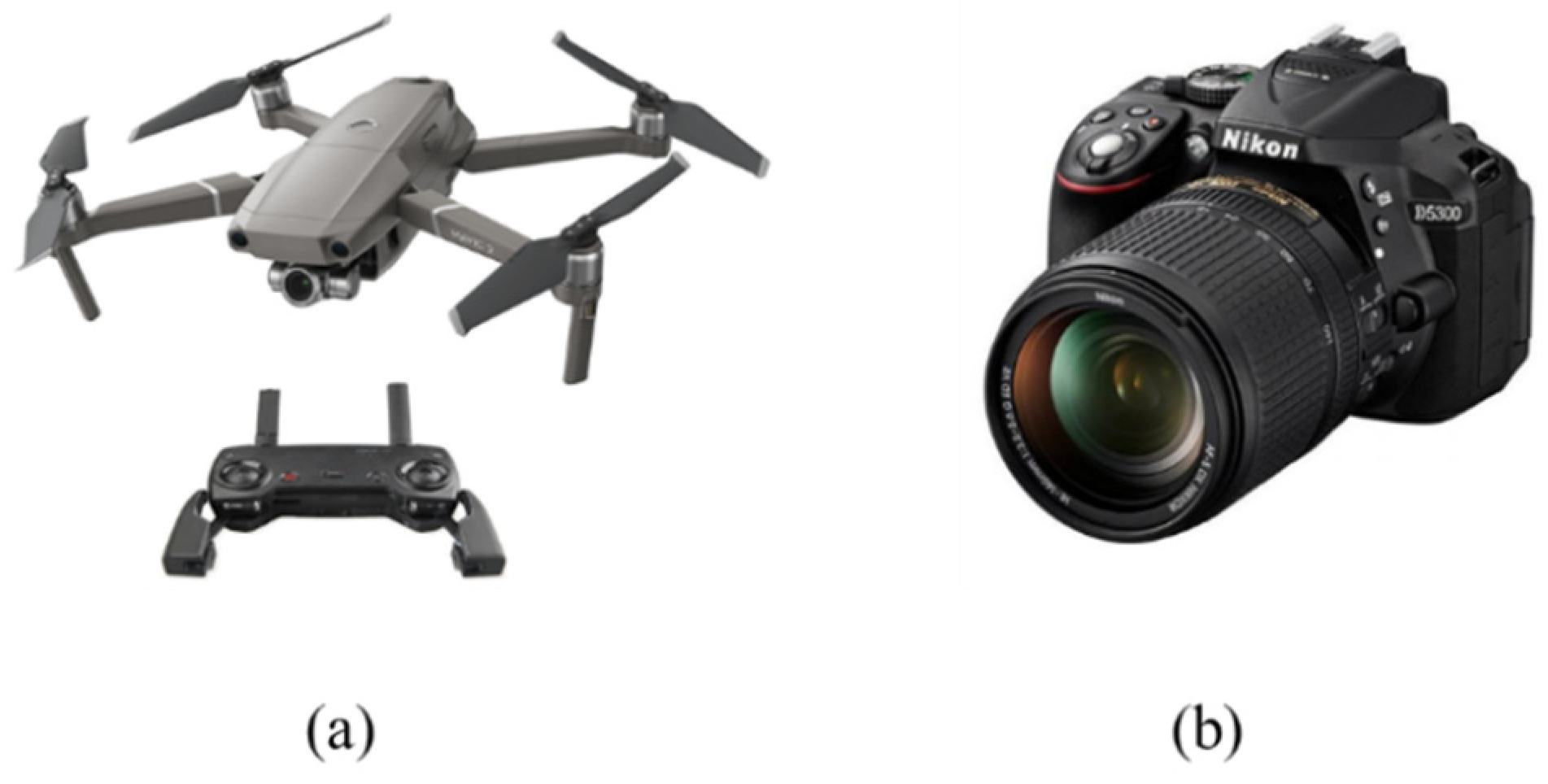
3.1. Equipment of Experiment

In this paper, the steel frame shown in Figure 3a is used as the bridge model for experiment, which has 9.8 m span, a width of 0.35 m, and a height of 0.35 m. The front plane of the bridge model (Figure 3b) has 56 nodes, which are used as the target points. The model is composed of hollow round bars (Figure 3c) and steel bolt balls (Figure 3d), in which the lengths of red and yellow hollow round members are 365 mm and 215 mm, respectively. The model is hinged at both ends as showed in Figure 3e. The top of the model is 1.4 m from the ground.

The bridge model is excited by a sudden concentrated load of 50 N for 5 times to collect the vibration signal, and the vibration time lasts for 80 s. The load is caused by an excitation hammer (Figure 3f) acting on the Node 43.

As shown in Figure 4, the tool used to collect bridge model video is a quad-rotor UAV (Mavic Air 2, Da-Jiang Innovations, Shenzhen, China) and a fixed camera (D5300, Nikon Corporation, Tokyo, Japan); the former has an image resolution of 3840 × 2160 and an acquisition frequency of 30 frames/s, and the latter has an image resolution of 1920 × 1080 and an acquisition frequency of 60 frames/s; both of them are located in the place 2 m away from the model [39] as shown in Figure 5.

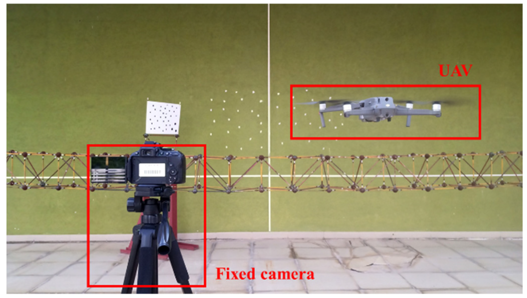
3.2. Experimental Scheme

This experiment is mainly divided into two parts:

(1)

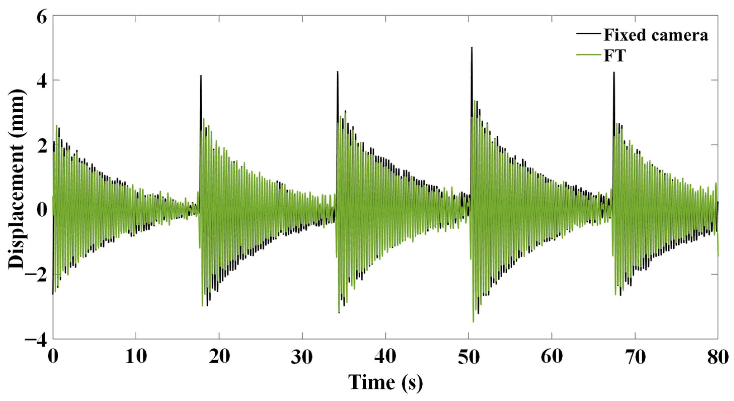
The displacement signal measured by the UAV is corrected by a filter combined FT with IFT in the first part. By comparing the correction results obtained by filtering different low-frequency signals $F$ and taking the degree of consistency with the displacement signal measured by the fixed camera as the index, the $F$ with best correction effect on the displacement signal measured by a UAV can be determined.

(2)

The processing effects of EMD, FT, and DF techniques on the displacement signal measured by the UAV and the extraction accuracy of modal parameters based on vibration signal are compared. The processing effects of three techniques are compared from three indexes: burr degree, correction accuracy, and consistency with the displacement signal measured by the fixed camera. Finally, the effect of three methods on identification of the modal parameters based on vibration signals are compared from the extracted natural frequency and mode shape of the model.

4. Experimental Results and Analysis

For better observation, the vibration signals of Node 15 are displayed.

4.1. Influence of F on the Correction Effect of FT

The original displacement signal collected by the UAV has a serious drift caused by the ego-motion of the UAV during the measurement, as shown in Figure 6. The displacement time–history curve measured by the UAV is converted into the spectrum by FT (Figure 7). The figure shows that there is a peak at about 3 Hz, which is caused by structural vibration and is also the part to be studied. Moreover, there are zero drift and many burrs near 0 Hz. The main cause of the burrs is the motion of the UAV during measurement, which is a kind of low-frequency irregular motion. In order to better study the structural vibration, the signal close to 0 Hz is removed, and then, the obtained new frequency domain signal is processed by IFT to obtain the time domain signal (Figure 8), that is, the structural vibration signal without false displacement caused by the ego-motion of the UAV.

In order to study the influence of $F$ on correction effect of FT, firstly, the value of $F$ is taken as 0.5, 1, 2 and 3 Hz, respectively. The corrected signals are shown in Figure 9 which shows that when $F=0.5\mathrm{Hz}$, the corrected signal has many burrs and is unstable. When $F=3\mathrm{Hz}$, even if the curve is smooth and there are few burrs, the characteristic of free vibration attenuation of displacement signal is not obvious. When $F=1\mathrm{Hz}$, although there are burrs in the curve, it tends to be stable. The main reasons are as follows: when $F$ is low, the low-frequency signals caused by the UAV ego-motion cannot be filtered out cleanly, resulting in poor correction effect; and when $F$ is high enough to approach the natural frequency of the structure of 3.281 Hz, some signals caused by the structural vibration may be filtered out, resulting in poor correction effect. Therefore, the value of $F$ is explored in the range of 1 Hz to 3 Hz to determine the value of $F$ with the best correction effect.

Although the burr degree of the curve decreases with the increase of $F$ between 1 Hz and 3 Hz, the free vibration attenuation characteristics of the obtained displacement curve gradually decrease, and therefore, the index for judging correction effect in this part is the degree of consistency with the displacement signal measured by the fixed camera. The degree of consistency between two displacement signals can be expressed by the Time Response Assurance Criterion (TRAC) [40]. Therefore, a high TRAC indicates a higher degree of similarity, that is, a better correction effect. The corrected signal of FT ($F=2\mathrm{Hz}$) and the measurement result of the fixed camera are shown in Figure 10. The relationship between $F$ and TRAC is shown in Figure 11, the ordinate of which is the average TRAC of the six nodes of the model with larger amplitude (Nodes 14, 15, and 16 and 42, 43, and 44) corresponding to $F$ (the subsequent TRACs mentioned in this paper are the average TRAC values of the six nodes with larger amplitude to ensure the reliability of the results). The figure shows that in the range of 1 Hz to 3 Hz, with increase of $F$, the TRAC first increases and then decreases. When the TRAC is the largest, $F$ is 1.7 Hz. Therefore, 1.7 Hz is regarded as the ideal $F$ value.

4.2. Comparison of EMD, FT, and DF

The processing effects of EMD, FT and DF techniques on the UAV measurement displacement signal and the effect of modal parameter extraction from the vibration signal are compared in this section. The true displacement of the bridge model can be decomposed from the original displacement signal by EMD (Figure 12a). The original signal contains seven IMFs and a remainder. The first IMF is the real displacement signal of the bridge model, which has obvious characteristics of free vibration attenuation. The decomposed remainder is monotonic, which is the condition to terminate the process of EMD. The signals shown in Figure 12a are processed by FT to obtain the corresponding spectrum diagrams (Figure 12b), which indicates that only the first IMF contain the structural vibration (frequency close to 3 Hz), which further indicates that IMF 1 is the real vibration signal of the structure. The decomposed components except IMF 1 are combined into a composite signal, which is the false displacement caused by the UAV measurement (Figure 13). The components of the original signal decomposed by EMD are reconstructed into a new signal. The standard deviation of the error curve between the new signal and the original signal is 3.687 × 10⁻¹⁵, indicating that the error of the EMD process is very small and negligible.

Since the signal measured by the UAV and corrected by DF is an acceleration signal, in order to facilitate comparison, the displacement signal measured by the fixed camera and the UAV displacement signal corrected by EMD and FT are processed by the second-order differential filtering, as shown in Figure 14. It shows that the curves of four cases are similar. In this section, the processing effects of three techniques are compared with three indexes.

The locally weighted regression (LOWESS [41]) can be used to smooth the original displacement signal to obtain the ideal displacement curve $x^{\prime }\left(t\right)$. The burr degree of the time–history curve can be reflected by the average value of the error curve between $x\left(t\right)$ and $x^{\prime }\left(t\right)$, which is defined as ECA in this paper. The higher the ECA, the more burrs the curve has. The average ECA of the six nodes of the model with larger vibration amplitude (Nodes 14, 15, and 16 and 42, 43, and 44) are shown in

Table 1. Indexes of three methods.

Method	EAC	TRAC	STD
EMD	24.897	0.941	98.604
FT	25.310	0.942	99.914
DF	26.456	0.918	106.508

(the subsequent ECAs mentioned in this paper are the average ECA values of the six nodes). It shows that the ECA of EMD is the lowest, followed by FT, which are 24.897 and 25.310, respectively; while, the ECA of DF is the highest, which is 26.456.

The TRAC between the corrected signals obtained by the three methods and the measurement results of the fixed camera are shown in Table 1. The TRAC of FT is the highest, which is 0.942, followed by EMD, which is 0.941, while the relative error of them is only 0.106%; the TRAC of DF is the lowest, which is 0.918.

The signals of a stationary point on the model background measured by the UAV and corrected by three methods are shown in Figure 15. Theoretically, the curves are straight lines, so the Standard Deviation (STD) reflects the accuracy of correction. The average STD values of six static points are shown in Table 1 (the subsequent STDs mentioned in this paper are the average STD values of six static points). It demonstrates that the STD of EMD is the lowest, followed by that of FT, and they are 98.604 and 99.914, respectively. The STD of DF is the highest, which is 106.508.

Figure 16 illustrates the PSD curves of the signals shown in Figure 14. According to the principle of OMA, the peak of the PSD curves corresponds to the modal natural frequency. The PSD curves obtained by the three methods have obvious peaks, and the extracted structural natural frequency is consistent with that extracted from the measurement of the fixed camera, indicating the good performance of the three methods in extracting the structural natural frequency.

Figure 17 shows the mode shape obtained from the acceleration signals of three correction methods and the fixed camera measurement. The modal assurance criterion (MAC) [42] is used to evaluate the fitting degree between the mode shape curves. The mode shape obtained by the fixed camera is taken as the reference, the MAC values of EMD, FT, and DF are 0.994, 0.986, and 0.981, respectively. Based on the above analysis, EMD is the best in the three correction techniques of signal measured by UAVs on processing effect and modal parameter identification of bridge models.

5. Discussion

The discussion is mainly divided into three parts:

(1)

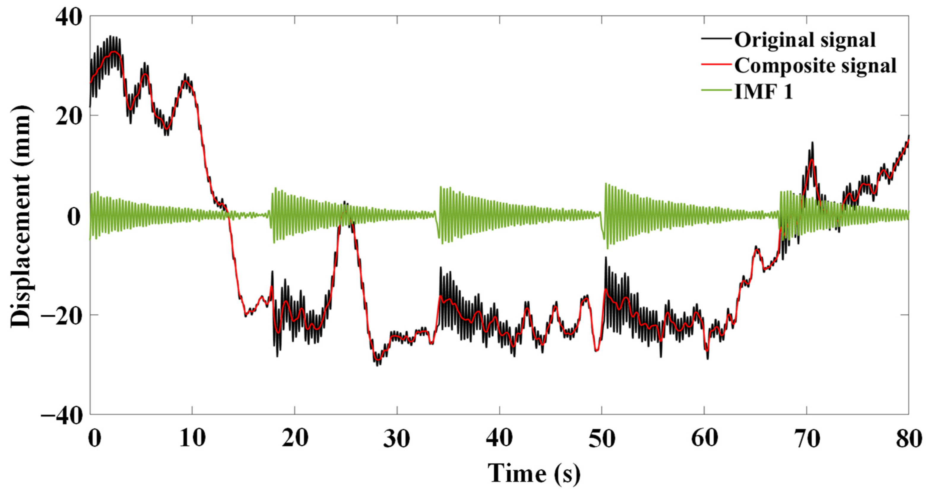
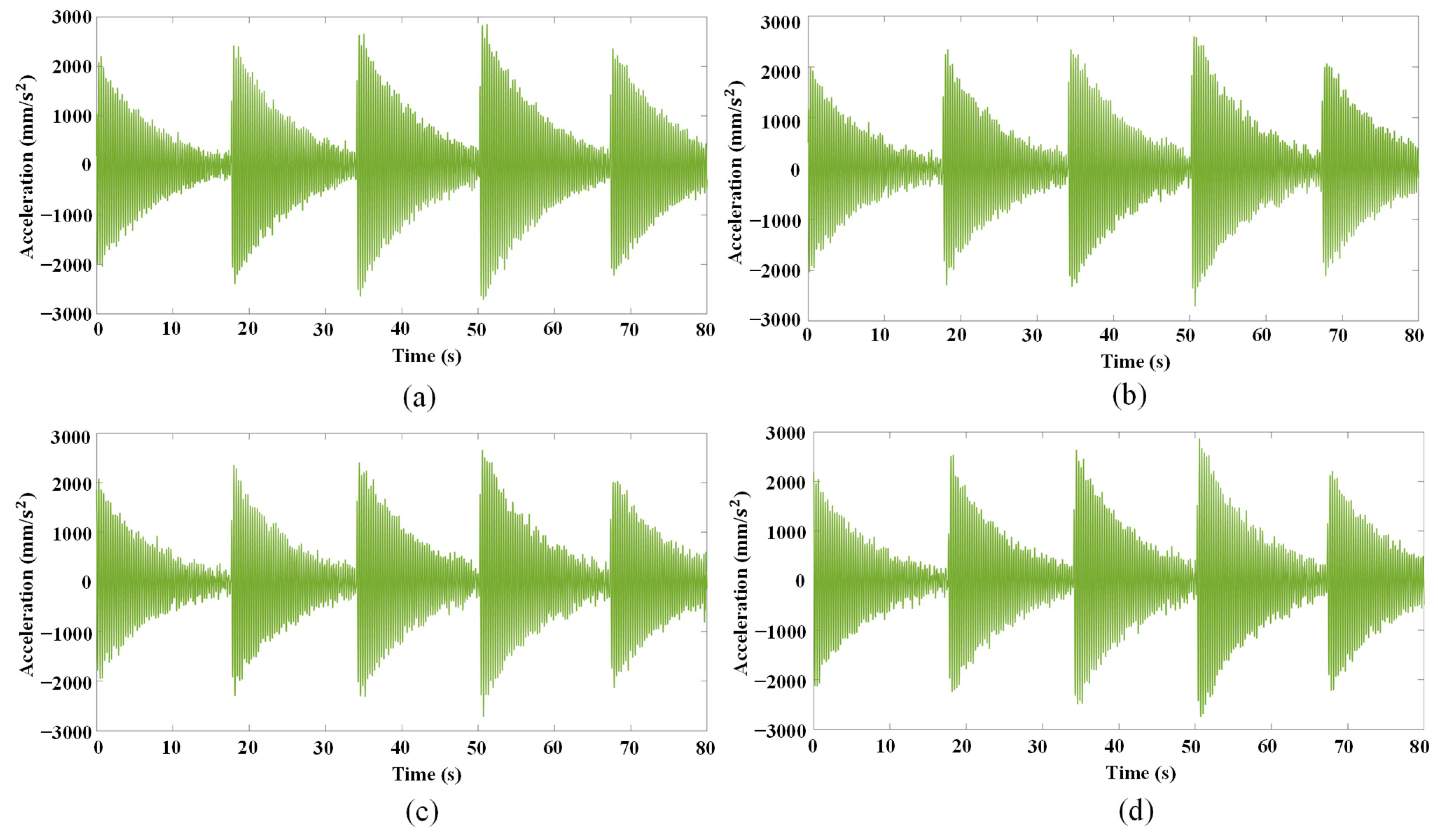
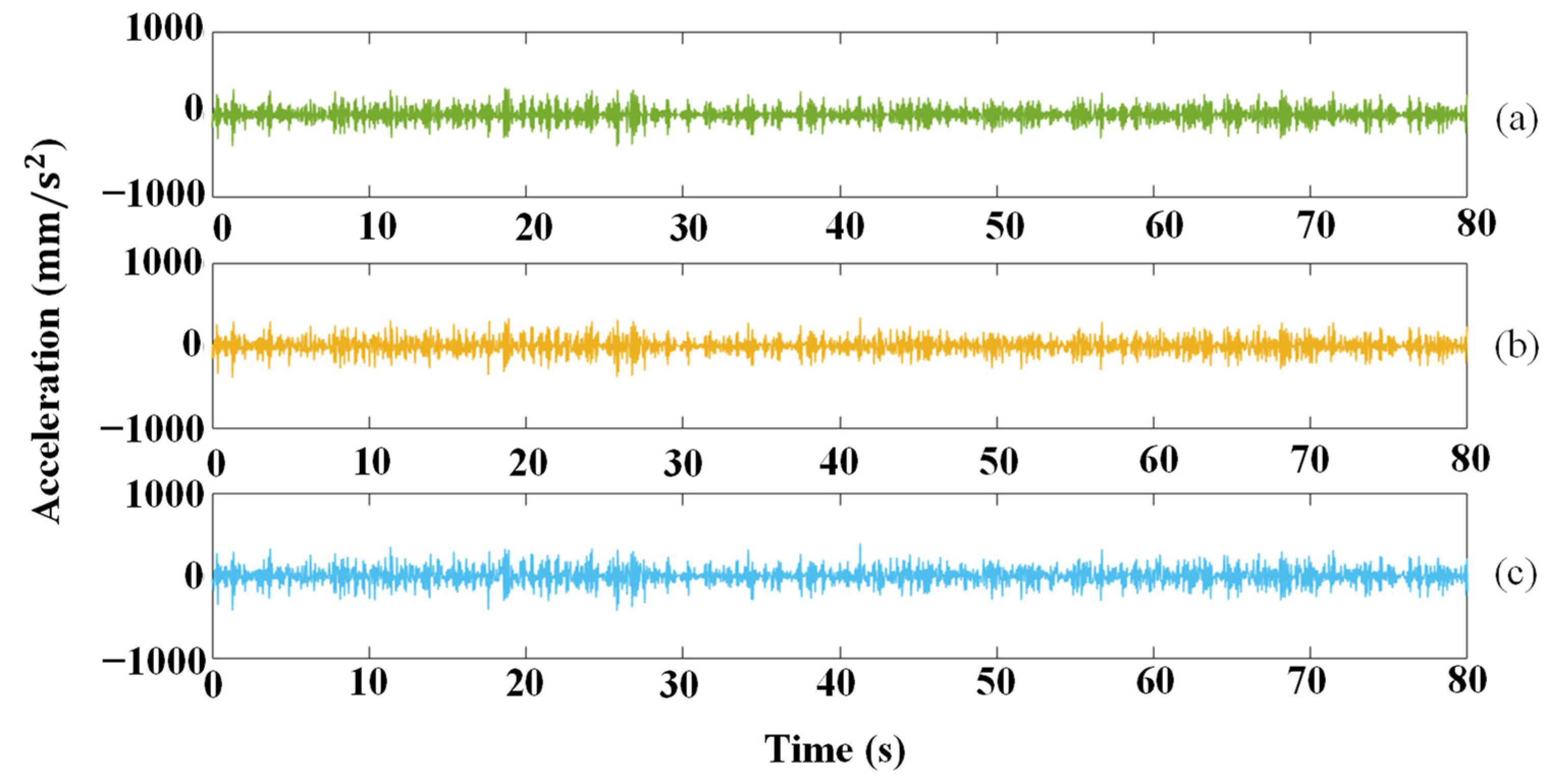
From the above experimental results, it can be known EMD has the best effect on the correction of displacement signal measured by the UAV. With respect of the acceleration signals, the effect of EMD and FT is better than DF, and the reason is as follows: the signals of EMD and FT are processed by second-order differential filtering on the basis of the corrected signals, while DF directly applies a differential filter to the original signal, which contains random signal caused by UAV measurement, so the signal after DF is poor. Figure 18 shows the EMD corrected displacement signal and its second-order differential. The figure shows that the burr of the signal increases significantly after DF, which shows the noise can be introduced by DF. Moreover, the true displacement signal of the bridge model cannot be obtained through DF, and therefore, EMD and FT are obviously more reliable for the processing of displacement signal measured by the UAV.

The comparisons of correction effect of EMD and FT based on the displacement signals are shown in

Table 2. Indexes of EMD, FT and DF.

Method	EAC	TRAC	STD
EMD	0.033	0.950	0.053
FT	0.045	0.946	0.062
DF	0.036	0.947	0.060

. It can be seen that EMD is better than FT, mainly because the high time resolution (the minimum time interval on the time axis) and the high frequency resolution (the minimum frequency interval on the frequency axis) cannot be obtained by FT at the same time, and the conversion between time domain signal and frequency domain signal is not accurate enough. In addition, with FT correction technique, it is not easy to find the optimal value of $F$ without knowing the natural frequency of the structure in advance, so EMD is more generally applicable than FT.

(2)

In addition to the above three techniques for signal measured by the UAV, Average Filtering (AF) [43] technique can also be used to correct the displacement signal measured by the UAV (see the Appendix A for more details). In the first step of AF correction technique, the signal of structural vibration is filtered out from the original signal, and the obtained displacement signal is the false displacement. In the second step, the filtered structural vibration signal can be obtained by subtracting the false displacement from the original signal. The correction effect of AF depends on $N$ (see the Appendix A for more details). The optimal effect of AF technique ($N=8$, it is verified by numerical experiment) and the correction effects of EMD and FT are compared in Table 2 (the results are based on the displacement signals). The table shows that the effect of AF technique is between EMD and FT. Therefore, using AF to correct the displacement measured by UAVs is also a considerable method.

During the processing of AF, partial false displacement signals may be filtered or partial structural vibration signals are not filtered cleanly, which may lead to poor correction effect. In addition, the value of $N$ is different for different data, so AF technique is not as applicable as EMD.

(3)

The above conclusion is based on the bridge model. In follow-up research, the methods used in this paper will be applied to the measurement results of actual bridges.

6. Conclusions

In this paper, two displacement correction techniques for UAV measurement are proposed, and the bridge modal parameters can be extracted accurately from the vibration signals obtained by the two correction techniques, EMD and FT. Since the correction effect of FT can be affected by the value of $F$, the optimal $F$ value must be determined before correction. The processing effects of EMD, FT, and DF on UAV signals are compared; the advantages of EMD in correcting UAV measured displacement signals are demonstrated. The static reference points are not required for the used two methods to correct the UAV measurement displacement. Unlike with DF, the signal obtained with the two methods is the displacement signal of the structure. Therefore, EMD and FT are very suitable for actual bridge measurement.

References

1. Doebling, S.W.; Farrar, C.R.; Prime, M.B. A Summary Review of Vibration-Based Damage Identification Methods. Shock Vib. Dig. 1998, 30, 91–105. [Google Scholar] [CrossRef]
2. Kovačič, B.; Kamnik, R.; Štrukelj, A.; Vatin, N. Processing of Signals Produced by Strain Gauges in Testing Measurements of the Bridges. Procedia Eng. 2015, 117, 795–801. [Google Scholar] [CrossRef]
3. Soyoz, S.; Feng, M.Q. Long-Term Monitoring and Identification of Bridge Structural Parameters. Comput. Civ. Infrastruct. Eng. 2010, 24, 82–92. [Google Scholar] [CrossRef]
4. Siringoringo, D.M.; Fujino, Y. Noncontact Operational Modal Analysis of Structural Members by Laser Doppler Vibrometer. Comput. Civ. Infrastruct. Eng. 2010, 24, 249–265. [Google Scholar] [CrossRef]
5. Psimoulis, P.; Pytharouli, S.; Karambalis, D.; Stiros, S. Potential of Global Positioning System (GPS) to measure frequencies of oscillations of engineering structures. J. Sound Vib. 2008, 318, 606–623. [Google Scholar] [CrossRef]
6. Shi, J.; Tomasi, C. Good Features to Track. In Proceedings of the IEEE Computer Society Conference on Computer Vision and Pattern Recognition (CVPR), Seattle, WA, USA, 21–23 June 1994; Volume 600, pp. 593–600. [Google Scholar]
7. Lucas, B.D. An Iterative Image Registration Technique with an Application to Stereo Vision (DARPA). In Proceedings of the 7th International Joint Conference on Artificial Intelligence, Vancouver, BC, Canada, 24–28 August 1981; Volume 81, pp. 674–679. [Google Scholar]
8. Liu, F.; Yundong, W.U.; Cai, G.; Chen, S.; Science, S.O.; University, J. Research of Feature Point Tracking Algorithm for UAV Video Image Based on KLT. J. Jimei Univ. 2017, 22, 73–80. [Google Scholar]
9. Zhu, J.; Lu, Z.; Zhang, C. A marker-free method for structural dynamic displacement measurement based on optical flow. Struct. Infrastruct. Eng. 2020, 18, 84–96. [Google Scholar] [CrossRef]
10. Han, S.H.; Rahim, T.; Shin, S.Y. Detection of Faults in Solar Panels Using Deep Learning. In Proceedings of the 2021 International Conference on Electronics, Information, and Communication (ICEIC) 2021, Jeju, Korea, 31 January–3 February 2021; pp. 1–4. [Google Scholar]
11. Choi, Y.J.; Rahim, T.; Ramatryana, I.N.A.; Shin, S.Y. Improved CNN-Based Path Planning for Stairs Climbing in Autonomous UAV with LiDAR Sensor. In Proceedings of the 2021 International Conference on Electronics, Information, and Communication (ICEIC), Jeju, Korea, 31 January–3 February 2021; pp. 1–7. [Google Scholar] [CrossRef]
12. Hassan, S.-A.; Rahim, T.; Shin, S.-Y. An Improved Deep Convolutional Neural Network-Based Autonomous Road Inspection Scheme Using Unmanned Aerial Vehicles. Electronics 2021, 10, 2764. [Google Scholar] [CrossRef]
13. Ellenberg, A.; Kontsos, A.; Moon, F.; Bartoli, I. Bridge related damage quantification using unmanned aerial vehicle imagery. Struct. Control. Health Monit. 2016, 23, 1168–1179. [Google Scholar] [CrossRef]
14. Hoskere, V.; Park, J.-W.; Yoon, H.; Spencer, B.F., Jr. Vision-Based Modal Survey of Civil Infrastructure Using Unmanned Aerial Vehicles. J. Struct. Eng. 2019, 145, 04019062. [Google Scholar] [CrossRef]
15. Rodríguez-Canosa, G.; Stephen, T.; Jaime, D.C.; Antonio, B.; Bruce, M. A Real-Time Method to Detect and Track Moving Objects (DATMO) from Unmanned Aerial Vehicles (UAVs) Using a Single Camera. Remote Sens. 2012, 4, 1090–1111. [Google Scholar] [CrossRef]
16. Soycan, A.; Soycan, M. Perspective correction of building facade images for architectural applications. Eng. Sci. Technol. Int. J. 2018, 22, 697–705. [Google Scholar] [CrossRef]
17. Wu, Z.; Chen, G.; Ding, Q.; Yuan, B.; Yang, X. Three-Dimensional Reconstruction-Based Vibration Measurement of Bridge Model Using UAVs. Appl. Sci. 2021, 11, 5111. [Google Scholar] [CrossRef]
18. Weng, Y.; Shan, J.; Lu, Z.; Lu, X.; Spencer, B.F. Homography-based structural displacement measurement for large structures using unmanned aerial vehicles. Comput. Civ. Infrastruct. Eng. 2021, 36, 1114–1128. [Google Scholar] [CrossRef]
19. Zhu, X.; Chen, Z.; Tang, C.; Mi, Q.; Yan, X. Application of two oriented partial differential equation filtering models on speckle fringes with poor quality and their numerically fast algorithms. Appl. Opt. 2013, 52, 1814–1823. [Google Scholar] [CrossRef] [PubMed]
20. Zhang, J.; Wu, Z.; Chen, G.; Liang, Q. Comparisons of Differential Filtering and Homography Transformation in Modal Parameter Identification from UAV Measurement. Sensors 2021, 21, 5664. [Google Scholar] [CrossRef] [PubMed]
21. Huang, N.E.; Shen, Z.; Long, S.R.; Wu, M.C.; Shih, H.H.; Zheng, Q.; Yen, N.-C.; Tung, C.C.; Liu, H.H. The empirical mode decomposition and the Hilbert spectrum for nonlinear and non-stationary time series analysis. Proc. R. Soc. Lond. Ser. A Math. Phys. Eng. Sci. 1998, 454, 903–995. [Google Scholar] [CrossRef]
22. Wang, G.; Chen, X.Y.; Qiao, F.L.; Wu, Z.; Huang, N.E. On Intrinsic Mode Function. Advances in Adaptive Data Analysis 2010, 2, 277–293. [Google Scholar] [CrossRef]
23. Rao, R.; Li, C.; Huang, Y.; Zhen, X.; Wu, L. Method for Structural Frequency Extraction from GNSS Displacement Monitoring Signals. J. Test. Eval. 2019, 47, 2026–2043. [Google Scholar] [CrossRef]
24. Bochner, S. Fourier transforms. In Annals of Mathematics Studies; Princeton University Press: Princeton, NJ, USA, 1949; Volume 7, pp. 145–151. [Google Scholar]
25. Lin, H.-C.; Ye, Y.-C. Reviews of bearing vibration measurement using fast Fourier transform and enhanced fast Fourier transform algorithms. Adv. Mech. Eng. 2019, 11, 1687814018816751. [Google Scholar] [CrossRef]
26. Lazaro, J.; Wessel, R.; Koppenborg, J.; Dudziak, G.; Blewett, I. Inverse Fourier transform method for characterizing arrayed-waveguide gratings. IEEE Photon Technol. Lett. 2003, 15, 93–95. [Google Scholar] [CrossRef]
27. Brownjohn, J.; Magalhaes, F.; Caetano, E.; Cunha, A. Ambient vibration re-testing and operational modal analysis of the Humber Bridge. Eng. Struct. 2010, 32, 2003–2018. [Google Scholar] [CrossRef]
28. Zhang, Y.; Zhang, S.; Li, H.; Wen, B. Harmonic mode identification in the operational modal analysis and its application. Zhendong Ceshi Yu Zhenduan/J. Vib. Meas. Diagn. 2008, 28, 197–200. [Google Scholar]
29. Yan, W.-J.; Ren, W.-X. An Enhanced Power Spectral Density Transmissibility (EPSDT) approach for operational modal analysis: Theoretical and experimental investigation. Eng. Struct. 2015, 102, 108–119. [Google Scholar] [CrossRef]
30. Yan, W.-J.; Ren, W.-X. Operational Modal Parameter Identification from Power Spectrum Density Transmissibility. Comput. Civ. Infrastruct. Eng. 2012, 27, 202–217. [Google Scholar] [CrossRef]
31. Mohanty, P.; Rixen, D.J. Identifying mode shapes and modal frequencies by operational modal analysis in the presence of harmonic excitation. Exp. Mech. 2005, 45, 213–220. [Google Scholar] [CrossRef]
32. Jiang, Z.; Yi, H. An Image Pyramid-Based Feature Detection and Tracking Algorithm. Geomat. Inf. Ence Wuhan Univ. 2007, 32, 680–683. [Google Scholar]
33. Harris, F.J. On the use of windows for harmonic analysis with the discrete Fourier transform. Proc. IEEE 1978, 66, 51–83. [Google Scholar] [CrossRef]
34. Wang, J.; Ye, Y.; Pan, X.; Gao, X. Parallel-type fractional zero-phase filtering for ECG signal denoising. Biomed. Signal Process. Control 2015, 18, 36–41. [Google Scholar] [CrossRef]
35. Devriendt, C.; Guillaume, P. The use of transmissibility measurements in output-only modal analysis. Mech. Syst. Signal Process. 2007, 21, 2689–2696. [Google Scholar] [CrossRef]
36. Devriendt, C.; Guillaume, P. Identification of modal parameters from transmissibility measurements. J. Sound Vib. 2008, 314, 343–356. [Google Scholar] [CrossRef]
37. Sutton, M.; Mingqi, C.; Peters, W.; Chao, Y.; McNeill, S. Application of an optimized digital correlation method to planar deformation analysis. Image Vis. Comput. 1986, 4, 143–150. [Google Scholar] [CrossRef]
38. Brincker, R.; Zhang, L.; Andersen, P. Modal identification of output-only systems using frequency domain decomposition. Smart Mater. Struct. 2001, 10, 441–445. [Google Scholar] [CrossRef]
39. Chen, G.; Wu, Z.; Gong, C.; Zhang, J.; Sun, X. DIC-Based Operational Modal Analysis of Bridges. Adv. Civ. Eng. 2021, 2021, 6694790. [Google Scholar] [CrossRef]
40. Chen, G.; Liang, Q.; Zhong, W.; Gao, X.; Cui, F. Homography-based measurement of bridge vibration using UAV and DIC method. Measurement 2020, 170, 108683. [Google Scholar] [CrossRef]
41. Cleveland, W.S. LOWESS: A Program for Smoothing Scatterplots by Robust Locally Weighted Regression. Am. Stat. 1981, 35, 54. [Google Scholar] [CrossRef]
42. Pastor, M.; Binda, M.; Harčarik, T. Modal Assurance Criterion. Procedia Eng. 2012, 48, 543–548. [Google Scholar] [CrossRef]
43. Zhang, C.; Xu, C.Y. A De-Noising Method of Acceleration Signal for Vehicle Based on Kalman Filter and Average Filter. Adv. Mater. Res. 2011, 225, 605–608. [Google Scholar] [CrossRef]
Figure 1. The process of EMD.
Applsci 12 08689 g001
Figure 2. Process of operational modal analysis.
Applsci 12 08689 g002
Figure 3. Experimental model: (a) bridge model; (b) plane model of bridge; (c) bolt connecting balls; (d) hollow round bar; (e) supports; (f) an excitation hammer.
Applsci 12 08689 g003
Figure 4. Signal acquisition equipment: (a) UAV; (b) fixed camera.
Applsci 12 08689 g004
Figure 5. Experimental layout.
Applsci 12 08689 g005
Figure 6. Displacement signal measured by the UAV.
Applsci 12 08689 g006
Figure 7. Processed signal of FT.
Applsci 12 08689 g007
Figure 8. Processed signal of IFT.
Applsci 12 08689 g008
Figure 9. Corrected signals of 4 cases: (a) F = 0.5   Hz ; (b) F = 1   Hz ; (c) F = 2   Hz ; (d) F = 3   Hz .
Applsci 12 08689 g009
Figure 10. Displacement signal measured by the fixed camera and corrected signal by FT ( F = 2   Hz ).
Applsci 12 08689 g010
Figure 11. The relationship between F and TRAC.
Applsci 12 08689 g011
Figure 12. The results of EMD: (a) components of the original signal; (b) spectrum diagrams of the components.
Applsci 12 08689 g012
Figure 13. Original signal, IMF 1 and composite signal.
Applsci 12 08689 g013
Figure 14. Acceleration signals of four cases: (a) fixed camera; (b) EMD; (c) FT; (d) DF.
Applsci 12 08689 g014
Figure 15. Corrected signals of static point of three methods: (a) EMD; (b) FT; (c) DF.
Applsci 12 08689 g015
Figure 16. PSD curves of four cases: (a) fixed camera; (b) EMD; (c) FT; (d) DF.
Applsci 12 08689 g016
Figure 17. The mode shape identified by four methods.
Applsci 12 08689 g017
Figure 18. The signals corrected by EMD: (a) EMD corrected signal; (b) Its second-order differential.
Applsci 12 08689 g018