A Comparison of Pooling Methods for Convolutional Neural Networks

Abstract

One of the most promising techniques used in various sciences is deep neural networks (DNNs). A special type of DNN called a convolutional neural network (CNN) consists of several convolutional layers, each preceded by an activation function and a pooling layer. The feature map of the previous layer is sampled by the pooling layer (that seems to be an important layer) to create a new feature map with condensed resolution. This layer significantly reduces the spatial dimension of the input. It always accomplished two main goals. As a first step, it reduces the number of parameters or weights to minimize computational costs. The second step is to prevent the overfitting of the network. In addition, pooling techniques can significantly reduce model training time and computational costs. This paper provides a critical understanding of traditional and modern pooling techniques and highlights the strengths and weaknesses for readers. Moreover, the performance of pooling techniques on different datasets is qualitatively evaluated and reviewed. This study is expected to contribute to a comprehensive understanding of the importance of CNNs and pooling techniques in computer vision challenges.

1. Introduction

Machine learning is the foundation of computer and other technology intelligence. It promotes more use of predictive analytics, which could also extract previous data predicting future actions, consequences, and patterns. Deep learning is a kind of machine learning which employs mathematical models relating to the human mind. DNNs can emulate extensive nonlinear interconnections between inputs and outputs. Their design methods create arrangements, which express the object as a layered combination of primitives. Many adaptations of several fundamental methods make up deep architectures. DNNs have gained popularity in recent years, and numerous models for a variety of applications have been presented. The models are further divided into five categories named convolution neural networks (CNN), restricted Boltzmann machines (RBM), auto encoders, sparse coders, and recurrent neural networks [1].

Neural network computational methods have evolved over the past half-century. In 1943, McCulloch and Pitts designed the first model, recognized as the linear threshold gate [2]. Hebbian developed the Hebbian learning rule approach for training the neural network. However, would the Hebbian rule remain productive when all the input patterns became orthogonal? The existence of orthogonality in input vectors is a crucial component for this rule to execute effectively [3]. To meet this requirement, a much more productive learning rule, known as the Delta rule, was established. Whereas the delta rule poses issues with the learning principles outlined above, backpropagation has developed as a more complicated learning approach. Backpropagation could learn an infinite layered structure and estimate any commutative function [4,5]. A feed-forward neural network is most often trained using backpropagation (FFNN). The most basic FFNN must have at least one hidden layer positioned between the input and output layers. Each pair of neurons in an FFNN has a non-cyclic and directed connection between them, as shown in Figure 1.

Figure 1. Feed-forward neural network architecture.

A weighted summation technique determines the flows in a multilayer FFNN so that each layer is fully interconnected to the next layer. The weights are chosen to maximize the discrepancy between the compared to the planned result activation patterns, which is the error function [6]. The learning method is normally carried out using the backpropagation approach by first tweaking the dimension of the weight and then adding a decent derivative of the error of reference to the last layer’s parameters. Various kinds of practical issues, such as object and face recognition, are challenging for FFNNs to handle [7].

1.1. Convolutional Neural Networks

CNNs were established to overcome the problem related to the implementation of FFNNs. CNNs can start making use of the input modality’s two-dimensional spatial limitations while somehow decreasing the quantity of system parameters in the training phase [8]. CNNs are among the most significant and effective forms of deep neural networks (DNNs) and are extensively employed for object segmentation and classification. Convolution, pooling, and fully connected layers constitute a CNN as three primary layers. These layers are engaged with certain spatial activities [9,10]. By using variable kernels in convolution layers to convolve the input image, CNNs produces feature maps. Typically, just after the convolution layer is created, the pooling layer is added. By using this layer, you can map your feature dimensions and hyperparameters. A flat layer and a fully connected layer are added after the pooling layer. The flat layer transforms the preceding layer’s data 2D feature map into a 1D feature map that fits the following fully connected layer [11].

1.2. Pooling

There are two pooling methods commonly used in CNNs. Local pooling is the first method to display feature maps by pooling data from small local regions (e.g., 3 × 3). The second is global pooling, which creates a scalar value representing the image from the feature vector for each feature across the feature map. This representation is obtained and categorized through fully connected layers. For example, a popular Dense Net network contains four local pooling layers in addition to one global pooling layer [12]. Pooling is a nonlinear process that enables outputs at a particular location to be aggregated within one value. This unique value is computed from the statistics of subsequent outputs, improving the accuracy and sensitivity of feature translation for smaller input data [13,14]. The pooling layer decreases gradually the input’s dimensions, minimizing the memory consumption to preserve the variables and optimize statistical performance [15,16,17]. Overfitting is also addressed in neural architectures with the use of pooling layers [18]. In convolution-based systems, pooling is an important step in reducing the dimensions of extracted features. Reducing the number of variables in the value sequence minimizes the dimensions of the feature map. It transforms general feature descriptions into actionable information by keeping the information relevant and removing unnecessary details. Pool operations offer a variety of services. By excluding the partial connections between the convolution layers, the pooling operation provides some spatially transformed representation and reduces the computational cost of the upper layers. Features extracted from the previous layer are sampled on this layer to generate multiple feature maps with limited resolution. The two key goals of the pooling layer are to reduce the number of parameters or weights, thereby reducing computational overhead and avoiding overfitting [19]. Only important information should be extracted and irrelevant information should be removed using the ideal pooling process. In fact, the pooling paradigm employed is essential in solving the computer vision challenge since the prime objective is to transform the combined visual features (mapped by convolution) into a meaningful representation. As a consequence, the pooling process is very important throughout many computer vision architectures. Pooling minimizes computation costs by reducing the resolution of the feature map while retaining the key aspects required to complete the task.

1.3. Selection of Articles for Review

The preliminary selection of papers was narrowed down with the assistance of Google Scholar. Several pooling-related keywords (such as attention-weighted pooling, feature aggregating, CNN pooling, pooling in computer vision, etc.) were used to find relevant studies. Although the majority of the publications that were found use previously known pooling techniques, the papers that propose novel pooling approaches were primarily found and selected for review. This provided us with a total of 95 publications, a number of which introduced new methods for pooling data and several of which used standard strategies for pooling related to computer vision tasks.

The main contribution of this study includes reviewing and discussing different kinds of standard and novel pooling methods proposed in the literature on computer vision with their advantages, limitations, and applicability in different circumstances. In our opinion, this review and comparative analysis can serve as a benchmark for employing pooling mechanisms in various computer vision analysis tasks.

Popular pooling methods and novel techniques are the two categories into which we have classified the pooling approaches. To make the best use of all these basic elements of a pooling scheme, some researchers are aiming to develop advanced pooling techniques. The purpose of this study is to keep readers informed of recent developments in pooling methods. This study also provides a platform for analyzing the strengths and weaknesses of all common pooling strategies.

2. Popular Pooling Methods

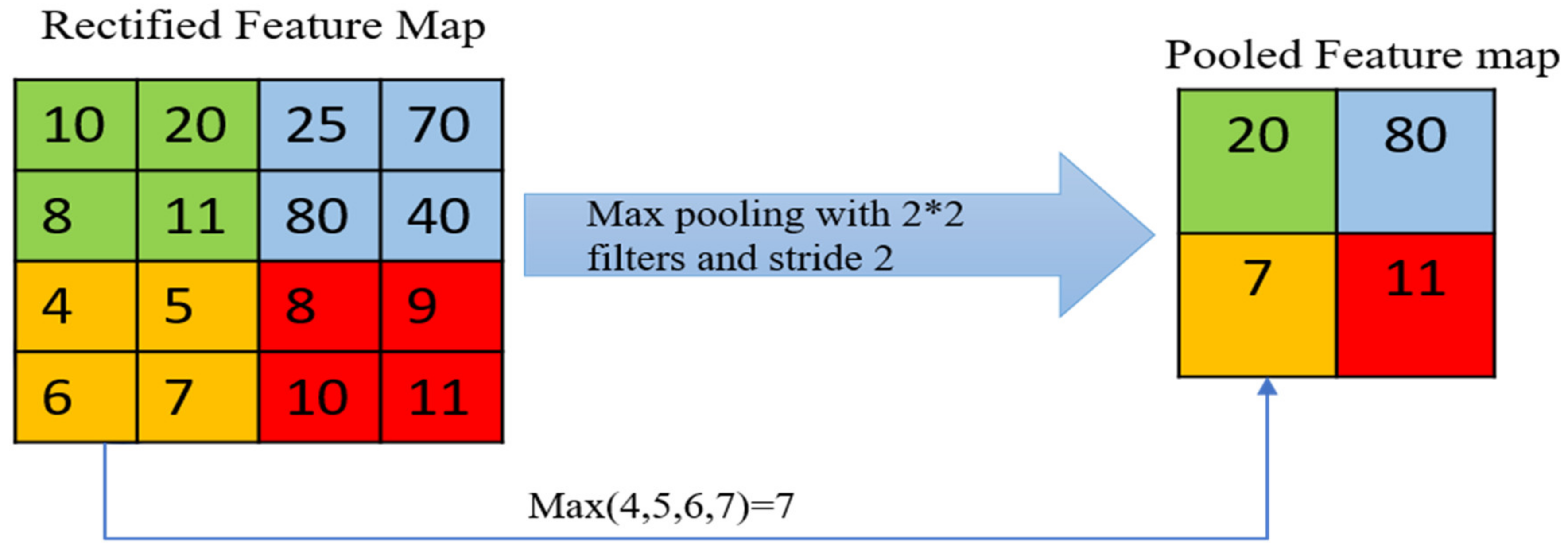
2.1. Max Pooling Method

The max pooling method [20] is simple and extensively applied in CNNs because there are no parameters that need to be tuned

Max pooling is a mechanism that optimizes the spatial size of a feature map while also providing the network with translation invariance. This is performed by exhibiting the greatest value in the feature map mainly within a k x k neighborhood. The max pooling technique identifies the biggest element in each pooling region [21,22]. Considering sparse codes and simple linear classifiers, max pooling shows better performance. Its popularity has increased in recent years as a result of the aforementioned factor. The equation for max pooling is:

$$f_{max}\left(X\right)=ma{x}_i{x}_i$$

(1)

𝐽 related filters are used for the composition of m-th max pooling band $pm=\left[p1,m,\dots .,pj,m,\dots .,pJ,m\right] ϵ R^J$:

$$pj,m=\max \left( h_j,\left(m-1\right)N+r\right)$$

(2)

Here, $N ϵ \{1,\dots ,R$} is termed as a pooling shift which allows enabling overlap within concerning pooling regions when $N<R$. The biggest limitation of max pooling is that all the other items are ignored completely whereas only the biggest element from the pooling region is assessed [23]. If most of the components in the pooling region are of large magnitude, the distinguishing traits vanish once the max pooling process has been completed. As a result of the loss of information, the scenario leads to unacceptably bad outcomes.

An example to further clarify the concept of max pooling operation is shown below in Figure 2, which depicts the input sample size of the pooling region as 4 × 4 while the filter size with a stride of 2 is 2 × 2. The first 2 × 2 parts (green) have a maximum value of 20 chosen by max pooling. The maximum value for each zone is selected accordingly and an output channel is created. The problem is that max pooling only considers the largest element and ignores the others, as we can see in the example. In some cases, after max pooling, salient features disappear when most elements have high magnitudes, which can lead to unacceptable results [24].

Figure 2. Max pooling operation illustration.

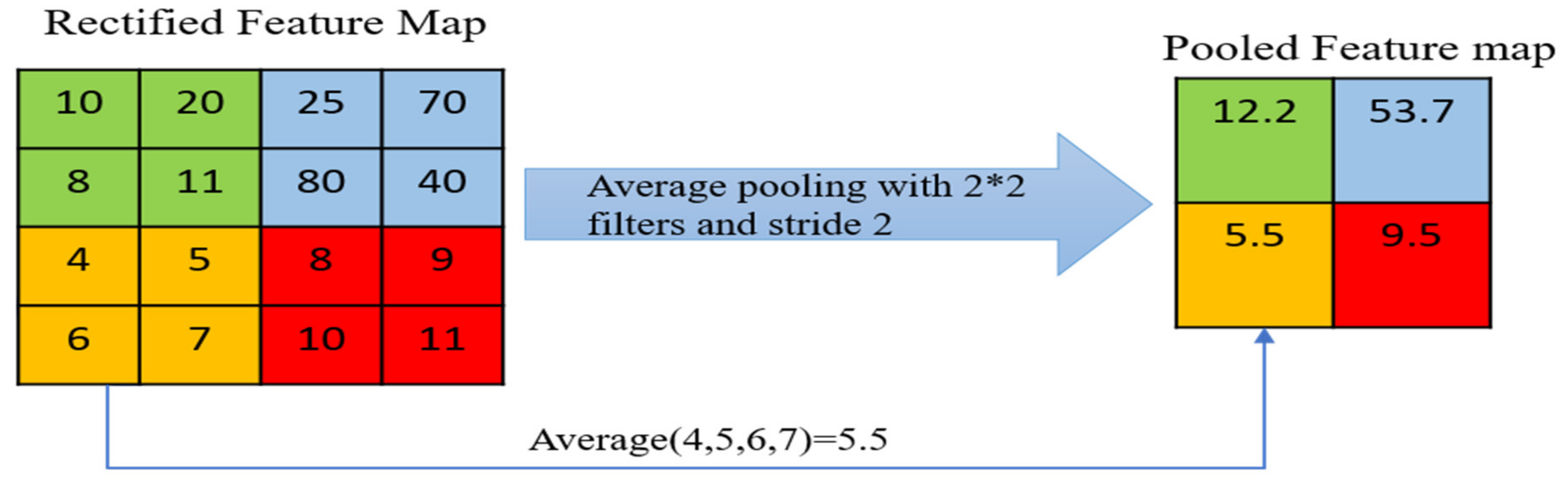
2.2. Average Pooling Method

The input is segmented into rectangular pooling areas, and an average pooling layer down samples by calculating the average values of each region. The implementation of the proposed idea was performed on the first convolution-based deep neural network [25]. Figure 3 provides a visual representation to clarify how the average pooling operation functions. In the average pooling strategy, the image input is divided into a number of separate rectangular boxes. The average of the values in each rectangle’s box is calculated and the output channel is presented. Average pooling is expressed mathematically as:

$$f_{ave}\left(X\right)=\frac{1}{N}{{\displaystyle \sum }}_i^N=1x_i$$

(3)

where x is a vector representing activations from a rectangular box of N permutations in an image or a channel (for example, the size of the rectangular area in Figure 3). The shortcoming seems to be mostly that this leads to a decline of information in terms of contrast. All of the activation values in the rectangular box are considered when estimating the mean. The estimated mean will indeed be low if the strength of all the activation functions is low, resulting in diminished contrast. The problem will worsen once most of the activations in the pooling zone have a zero value. In that situation, the convolutional feature characteristic would be reduced significantly [26].

Figure 3. Common pooling method demonstration.

Since neither the approaches of max nor average pooling consistently performs better than the other, different methods have been proposed that combine the advantages of max pooling and average pooling. In this research area, max pooling and average pooling are directly combined with weights and soft pooling. These algorithms add more parameters than max average pooling, which requires more time to learn or tune the parameters, and computational overhead increases [27].

2.3. Mixed Pooling Method

Max pooling only obtained the highest value from the designated pooling zone However, by integrating non-maximal activation, average pooling decreases the activation. In mixed max average pooling [28], the max pooling and the average pooling are simply merged with weights to take both into account, which overcomes the concerns with the max and average pooling discussed in Section 2.1 and Section 2.2. Yu et al. presented a hybrid approach that combined max and average pooling to fix this challenge [14]. Dropout and drop connect have quite a significant and negative effect on this approach. Equation (4) can be used to define mixed pooling.

$$Sj=\lambda max{a}_i+\left(1-\lambda \right)\frac{1}{\left|Rj\right|}{\displaystyle \sum }_{i\in Rj}{a}_i$$

(4)

Here, the choice between max pooling versus average pooling, λ, will be used. The value of $\lambda$ is considered as 0 or 1, which is chosen randomly. When the value of $\lambda$ is equal to zero, it behaves like an average pooling and when the value of $\lambda$ is 1 it behaves like a max pooling. The value of $\lambda$ would be saved for further use in forwarding propagation or also utilized during the backpropagation process. Numerous researchers have already shown its dominance over max and average pooling by employing image classification for a wide range of applications [29,30]. Yu et al. used three different datasets and proved mix pooling provides better results as compared to the max and average pooling. The main drawback of this pooling scheme is unresponsive behavior due to the fixed mixing ratio, which makes this hybrid approach insensitive towards the important features [31].

2.4. Tree Pooling

Convolutions are comparable to weighted average pooling because they incorporate filters that are learned during training. Tree pooling [32] learns how to combine a range of filters. The data from the pooling filters is used in this pooling strategy to perform learning of pooling activities, perform complementary learning, and reasonably combine these learned filters. A tree structure with leaf nodes can perform both learning processes [33]. Each leaf node (child node) in these “tree-like” representations is associated with a “grouping filter” that has a grouping area ($X ϵ R^N$) and is represented by ($V_m ϵ R^N$) where m is the identifier of the node.

$$fm\left(x\right)=\left\{\begin{array}{c}{V}_M^T X \left(if leaf node\right)\\ б\left(W_M^T\right) F_{\begin{array}{c}m, left \left(X\right)\\ 1\end{array}}+(1-б\\ \end{array}\right.\left( w_{M \left(x\right)}^T\right), right \left(X\right)$$

(5)

With this alone, backpropagation from all perspectives using traditional decision trees is not feasible. Each of these elements drives a single element in the tree pooling with a sigmoid “gate” function that allows the tree pooling to be distinguished when converting the input to useful outputs and their parameters. In terms of performance, tree pooling outperforms max [Section 2.1], average [Section 2.2], and mixed max average pooling [Section 2.3], however, tree pooling seems to have more parameters to learn when compared with mixed max and average pooling [34]. Blonder et al. demonstrated through their experiment that tree pooling is effective at the lower network layer focused on functional response [35].

2.5. Stochastic Pooling Method

Overfitting is a serious problem when training CNNs with fewer data. Various forms of pooling methods have been introduced to reduce overfitting, including mixed pooling [28], stochastic pooling [36], rank-based random pooling [37], max pooling dropout, and fractional max pooling. A trained model can be viewed as a set of networks connected as a result of randomization during training, with each random pool configuration defining a unique member of the group. The idea of stochastic pooling was presented by Fergus and Zeiler [38], inspired by dropouts [39]. Stochastic pooling is introduced to address the shortcomings of average and max pooling. Multinomial distribution is applied by stochastic pooling to pick the value randomly. In stochastic pooling, the probabilities’ pi values are constantly defined by normalized activations within the sectors for each region j. The description can be seen in the equation below.

$$pi=\frac{a_i}{\sum kϵR_J{a}_k}$$

(6)

By finding these probabilities, multinomial distribution will be created which determines a location and corresponds to the activation $a_l$ grounded on p. The location $l$ will be selected by multinomial distribution within the region.

$$s_j=a_l \mathrm{where} l~p \left(p_{1,\dots ,p\left|R_j\right|}\right)$$

(7)

In short, activations are selected based on probabilities and further calculated by multinomial distribution. The constraint on exclusively applying non-negative activation is stochastic pooling’s primary problem. Additionally, it is clear from the equation that the technique does not work for negative activations. Only the ReLU activation function is applied with stochastic pooling because the ReLU activation function lowers negative activations to zero. Stochastic pooling is still sensitive to overfitting, particularly if the training data are few [40]. This is because stochastic pooling is significantly more likely to generate strong activation during training, raising concerns about the possibility of overfitting. Therefore, rank-based stochastic pooling [41] presents a novel approach for estimating the likelihood based on the rankings of the activations inside each pooling region. All of these stochastic pooling problems involve scale-related challenges [42]. The working of stochastic pooling is depicted in Figure 4.

Figure 4. Stochastic pooling: a random sample is selected from a multinomial distribution of activations based on probabilities estimated by normalizing the activations. The chance of being selected increases with the size of the activation. In this figure, there are two activations, 1.6 and 2.4, with probabilities of 40% and 60%, respectively. However, 1.6 was chosen as the sampling activation despite the high probability of 2.4. Stochastic pooling can lose essential features because there is no way to predict which part of the input will be selected. Enhanced and regenerated from [43].

2.6. Spatial Pyramid Pooling Method

Spatial pyramid matching (SPM) is another term used for pyramid pooling. This pooling method has the unique ability to eliminate the requirement of fixed size image [44,45], which is the essential requirement in standard CNNs [46]. Fully connected layers apply fixed-size constraints instead of convolutional layers. Prior to the innovation of pyramid pooling for fitting images to CNNs, cropping and warping were the only techniques for resizing images. However, image cropping [38] and warping [47] each have different effects, leading to content loss and geometric distortion, respectively. The SPP layer is positioned on top of the final convolution layer to prevent the engagement of cropping and warping, which creates a new network named as SPP-net [48]. Spatial pyramid pooling (SPP) is considered to be a cutting-edge methodology for assessing pooling layer efficiency [49]. The SPP layer is designed to match the size of the feature maps in the SPP network, and the number of spatial bins remains constant at each pyramid level. Container sizes may vary. Using an image of size 128 × 128 and the four container numbers at the bottom of the pyramid can create a patch of size 32 × 32. Since there are 16 bins in total, the highest value within each bin is chosen as the activation value for the second level of the pyramid. The SPP layer generates a vector with a fixed dimension and fixed length as an outcome of pooling the activations for each bin, which is comparable to the product of the number of filters in the last convolutional layer and the number of bins in the SPP layer. As a result, the SPP technique can generate an output with a fixed length without taking the input’s size into account. Moreover, the SPP’s testing and training phases allow for adaptation to the input image scales, which strengthens the scale-invariance property and eliminates the overfitting problem in the network [50]. However, instead of going into various pooling functions or incorporating learning, spatial pyramid pooling is primarily designed to deal with images of variable sizes and can result in a more complicated learning procedure, resulting in less efficient output, such as a 16:89 percentage error rate on unaugment CIFAR10 [51].

3. Novel Pooling Methods

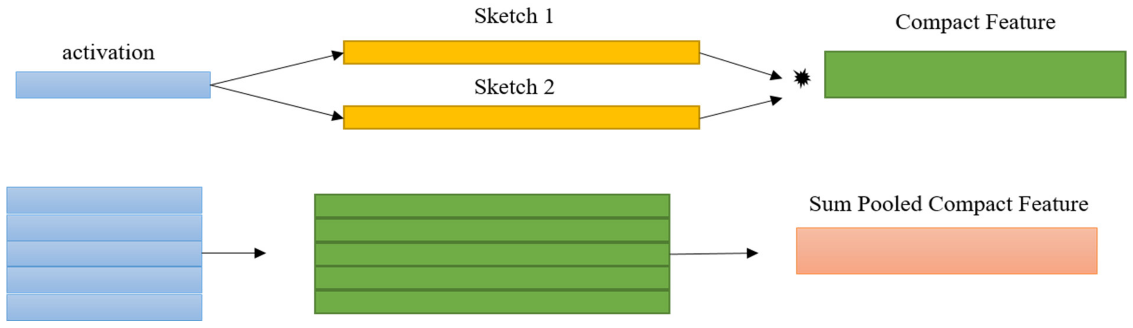
3.1. Compact Bilinear Pooling

Bilinear methods have been shown to perform well on several visual tasks, including semantic segmentation, fine-grained classification, and facial detection. End-to-end backpropagation is being used to train the compact bilinear pooling technique that allows for a low-dimensional and highly discriminatory image representation. This approach of pooling is also employed in [52,53].

For the last convolutional feature, this strategy is suggested to achieve global heterogeneity and rich representations, which attained cutting-edge performance in several multidimensional datasets. However, since computing pairing interaction between channels produces great complexity, dimension reduction methods have been presented. Low-rank bilinear pooling (Figure 5) shows a schematic representation of compacted bilinear pooling. End-to-end backpropagation has been used to train this pooling technique, which allows for a low-dimensional yet highly discriminatory image representation.

Figure 5. Image identification using the compact bilinear pooling method.

3.2. Spectral Pooling

Ripple et al. [54] proposed a novel pooling approach that included the concept of dimension reduction by shrinking the frequency domain representation of the data. Let h*w be the appropriate output feature map parameters and let x Rm*m be the given input map. The given input map is first treated with a discrete Fourier transform (DFT) after during which a frequencies representation submatrix of h*w size is eliminated from the center. Finally, inverse DFT is used to convert the h*w submatrix back into image pixels. By implementing a threshold-based filtering methodology, spectral pooling retains more information over max pooling for the very same output dimension. It fixes the problem of the output map’s dimensions being reduced significantly.

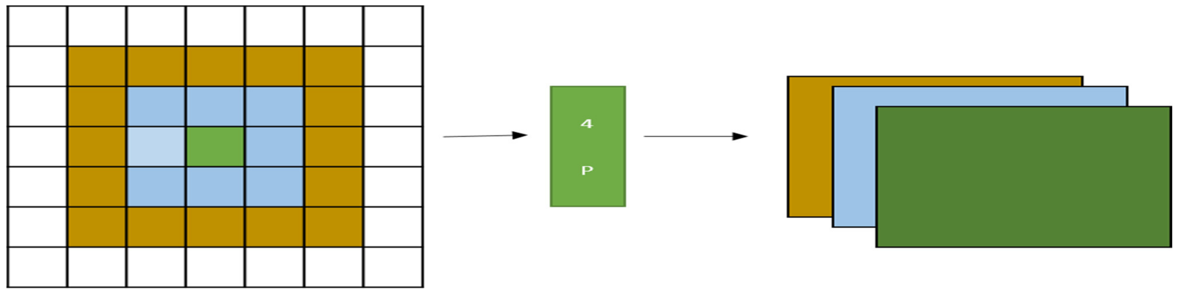
3.3. Per Pixel Pyramid Pooling

To obtain the requisite receptive field size, a wider pooling window could have been used as contrasted to a stride and a narrow pooling window. While using a large single pooling window, finer details may be lost. As a consequence, successive pooling with various window dimensions is conducted, and the results are concatenated to construct additional feature maps. The material from broad to fine scales is presented in the feature maps that emerge. The multi-scale pooling process can be carried out by each pixel without strides. The preceding is the formal definition of per-pixel pyramid pooling [55].

P^4p (F, S) = [P (F, S1)… P (F, S_m)]

P (F, Si) is a pooling process with a size of Si and a stride of 1, and s is a vector with an element count of M. To be clear, one channel of the extracted features is shown in Figure 6 to demonstrate the pooling process; the other channels obtained similar findings.

Figure 6. Representation of the 4P module with the pooling size vector s = [5, 3, 1].

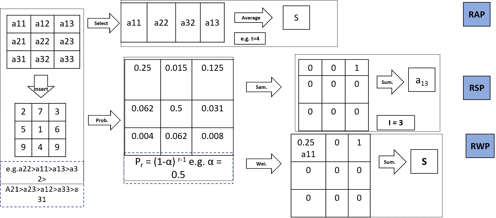
3.4. Rank-Based Average Pooling

The proposed pooling evaluates the average performance for practically zero negativity activation functions, which could also cause the loss of racist and discriminatory data by downplaying higher activation levels. Likewise, in max pooling, non-maximum activations are eliminated, leading to data loss. A rank-based average pooling layer can overcome the challenges of information loss imposed on both max pooling and average pooling layers (RAP) [56]. The outcome of the RAP can be stated as Equation (8):

$${\mathrm{S}}_j=1÷t{{\displaystyle \sum }}_{iϵR_{j, r_{i<t}}}^n{a}_i$$

(8)

The ranks boundary, which defines the categories of activations used during averaging, is represented by t. In feature maps, R stands for the pooling regions j, and t stands for the index of each activation inside of it. S_j and a_i, within this order, reflect the rank of activation I and the value of activation I. When t = 1, max pooling is established. According to Shi et al. [37], limiting t to a median value achieves good performance and a good balance between max pooling and average pooling. Therefore, RAP has better discriminative power than traditional pooling methods and is a perfect combination of maximum and average pooling. Figure 7 depicts a simulation of rank-based pooling in operation.

Figure 7. Rank-based average pooling: rankings are presented in ascending order, and activations for a pooling area are listed in descending order. The pooling output is calculated by averaging the four largest activations, since t = 4.

3.5. Max-Out Fractional Pooling

The concept of fractional pooling applies to the modification of the max pooling score. In this case, the multiplication factor (α) can only take non-integer values such as 1 and 2. The location of the pooling area and its random composition are, in fact, factors that contribute to the uncertainty provided by the largest max pooling. The region of pooling can be designed randomly or pseudo-randomly, with overlaps or irregularities, employing dropout and trained data augmentation. According to Graham B. et al. [57], the design of fractional max pooling with an overlapping region of pooling demonstrates greater performance than a discontinuous one. Furthermore, they observed that the results of the pooling region’s pseudo-random number selection with data augmentation were superior to those of random selection.

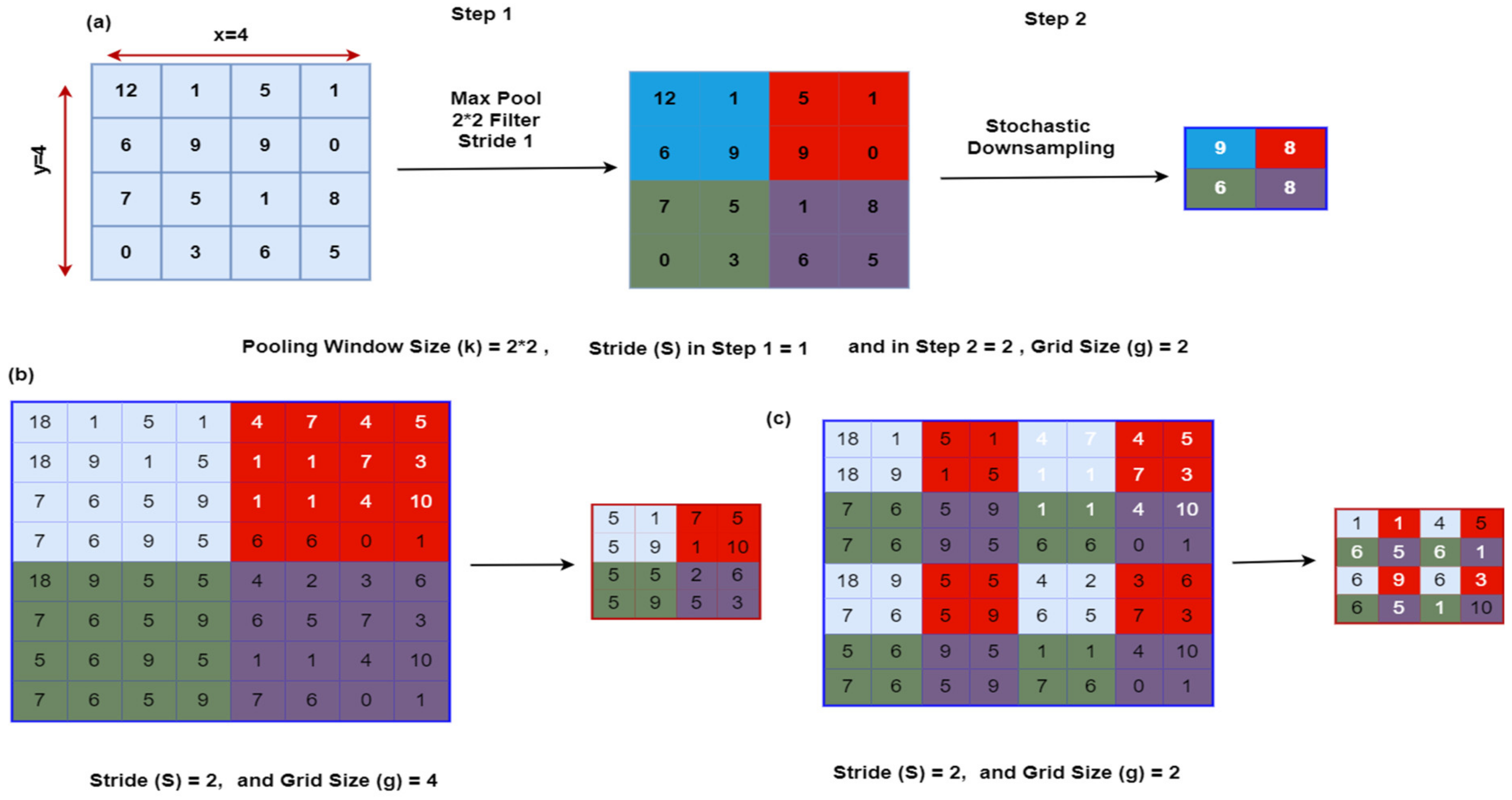
3.6. S3Pooling

Zhai et al. in 2017 presented the S3Pool method, a novel approach to pooling [58]. The pooling process is performed under this scheme in two stages. On each one of the preliminary phase feature maps (retrieved from the convolutional layer), the execution of max pooling is performed by stride 1. The outcome of step 1 is down sampled using a probabilistic process, in comparison to step 2, which first partitions the feature map of size X × Y into a preset set of horizontal (h) and vertical (v) panels. V is y/g and H is x/g. The following figure illustrates a schematic of S3Pooling. The working of S3 pooling is referred in Figure 8.

Figure 8. Working of S3 pooling mechanism. The dimension of the feature map in this example is 4 × 4, with both x and y = 4 represented in (a). The max pooling operation in step 1 uses stride 1, and there is no padding at the border. The grid size and stride should both be 2 in step 2. There will be two horizontal (h) and vertical (v) strips. In step 2, a stochastic downsampling is used to represent the rows and columns that were randomly chosen to build the feature map. Flexibility to change the grid size in step 2 in order to control the distortion or stochasticity is represented in (b,c).

Xu et al. [59] executed tests for the CIFAR-10, CIFAR-100, and SIT datasets using both network in the network (NIN) and residual network architectures to test the effectiveness of S3Pool in comparison to other pooling techniques (ResNet). According to the experimental observations, S3Pool showed better performance than NIN and ResNet with dropout and stochastic pooling, even when flipping and cropping were used as data augmentation techniques during the testing phase.

3.7. Methods to Preserve Critical Information When Pooling

Improper pooling techniques can lead to information loss, especially in the early stages of the network. This loss of information can limit learning and reduce model quality [60,61]. Detail-preserving clustering (DPP) [62] and local importance-based clustering (LIP) [63] minimize potential information loss by preserving key features during pooling operations. These approaches can also be known as soft approaches. Large networks require a lot of memory and cannot be started on devices with limited resources. One way to solve this problem is to quickly down sample to reduce the number of layers in the network. Poor performance may be the result of information loss due to the large and rapid reduction of the feature maps. RNNPool [64,65] attempts to solve this problem using a recursive down sampling network. The first recurrent network highlights feature maps and the second recurrent network summarizes its results as pooling output.

4. Advantages and Disadvantages of Pooling Approaches

The upsides and downsides of pooling operations in the numerous CNN-based architectures is discussed in Table 1, which would help researchers to understand and make their choices by keeping in mind the required pros and cons. Max pooling has indeed been applied by several researchers owing to its simplicity of use and effectiveness. Detail analysis was performed for further clarification of the topic.

Table 1. Advantages and disadvantages of different pooling approach in CNN.

Type of Pooling	Advantages	Drawbacks	References
Max Pooling	- Performs more effectively when integrated with simple classifiers and sparse code. - It complements sparse representations due to statistical features. - Eradicating no maximal elements might expedite calculation for upper layers.	- Deterministic in spirit. - The distinguishing characteristics vanish when the majority of the elements in the pooling region are available in significant magnitudes.	[38,39]
Average Pooling	- Easily understandable. - Execution is uncomplicated.	- Forthcoming in spirit. - If minor magnitudes are considered, the contrast is reduced.	[37,38,40,41,42,43,44,45,46,47,48,49,50,51,52,53,54,55,56,57,58,59,60,61,62,63]
Gated Max Average	- Responsive in style. - It is adaptive in whether the volume fraction can fluctuate based on the properties of the pooling region.	- Produces additional training parameters.	[41]
Mixed Max Average	- Stochastic pooling. - Facilitates in the problem of overfitting avoidance.	- Once it has been learned, the mix proportion does not really respond and adapt to the attributes of the region being integrated.	[42]
Pyramid Pooling	- Flexibility to manage input of any size. - Spatial bins with multiple levels. - Responsiveness to the image scales of an input.	- Deep networks’ training step involves complex implementation.	[43]
Stochastic Pooling	- Stochastic procedure. - It is conceivable to use non-maximal activations. - Feasibility of integrating any regularization method, including dropouts, data augmentation, loss tangent, etc. - There seems to be no hyper-parameter to specify. - Lower computational complexity.	- Complicated to interpret. - Extraneous to words negative activations. - Due to the lack of training data, overfitting occurs because strong activations primarily work in process updating. - Scaling challenge.	[44]
Tree Pooling	- Flexible to adapt in nature. - Differentiable in perspective among both parameters as well as inputs. - Effective at the network’s lower tiers.	- Inefficient due to thick layers of the network.	[41,66]
Fractional Max Pooling	- Stochastic method. - Choice of the pooling region via pseudo-randomness or randomness. - Appropriate use of data augmentation and pseudo-random selection. - Overlapped rather than disjointed fractional max pooling proved to be more efficient.	- Arbitrarily selecting the pooling zone significantly affects model performance in addition to data augmentation. - The disjointed fractional max pooling leads to significant degradation.	[36]
S3Pool	- Simple to learn and use. - Rapid computations while training. - Extrudes in the extent of distortions. - Implement data augmentation at the levels of the pooling layer to give it strong generalization performance. - Compared to max pooling, considerably increases the computational burden.	- Depending on the design for which it is being employed, the grid size should be adequately specified in each pooling layer. - A greater grid size potentially results in increased testing error.	[37]
Rank-Based Average Pooling	- For object recognition tasks, it is implemented. - It empowers us to reuse the convolution network’s feature map. - It provides an opportunity to train object detection systems from beginning to end, significantly shortening test and training periods.	- Performance issues can arise while generating lots of regions of interest. - Computing frequency falls short of the expectations. - End-to-end training, or training each aspect of the system in one go, is not practicable but could produce much-enhanced results.	[45]

Performance Evaluation of Popular Pooling Methods

The performance among the most latest pooling methods has been investigated systematically for the purpose of image classification in this section. We would like to emphasize that the primary aim of this study is to fairly assess the influence of the pooling strategies in the CNNs, not to establish the optimum classification architecture. Table 2 evaluates the effectiveness of different pooling approaches on standard datasets including MNIST, CIFAR-10, and CIFAR-100. The architecture and the forms of activation functions that have been used to implement these techniques are presented in the following table. In Table 2, it is shown that for the MNIST dataset, average pooling performed the worst, with an error rate of 0.83%. Furthermore, in comparison to other pooling methods, gated pooling was a significant improvement where the average and maximum pools were responsively combined. With a difference of 0.01%, mixed, tree max average pooling, and fractional max pooling were followed in order by the performance of gated pooling. These pooling strategies’ outstanding regularization and generalization capabilities were validated by their effective implementation. In conclusion, the NIN and max out networks’ respectively showed a strong performance and error frequencies of 0.45% and 0.47%. Unfortunately, their performance was still inadequate to what was achieved while pooling methods. It was found that for MNIST datasets, using the same network with ReLU activation, rank-based pooling (RSP) gave a higher error rate than the error rate provided by random pooling in the range of 0.42% to 0.59%.

Table 2. Comparing performance of various pooling methods on different standard datasets.

Pooling Methods	Architecture	Activation Function	Error Rate of Different Datasets			Accuracy	Reference
			MNIST	CIFAR-10	CIFAR-100
Gated Method	6 Convolutional Layers	RELU	0.29	7.90	33.22	88% (Rotation Angle)	[32]
Mixed Pooling	6 Convolutional Layers	RELU	0.30	8.01	33.35	90% (Translation Angle)
Max Pooling	6 Convolutional Layers	RELU	0.32	7.68	32.41	93.75% (Scale Multiplier)
Max + Tree Pooling	6 Convolutional Layers	RELU	0.39	9.28	34.75
Mixed Pooling	6 Convolutional Layers (Without data Augmentation)	RELU	10.41	12.61	37.20	91.5%	[34]
Stochastic Pooling	3 Convolutional Layers	RELU	0.47	15.26	42.58	---------	[36]
Average Pooling	6 Convolutional Layers	RELU	0.83	19.38	47.18	---------
Rank-Based Average Pooling (RAP)	3 Convolutional Layers	RELU	0.56	18.28	46.24	---------	[37]
Rank-Based Weighted Pooling (RWP)	3 Convolutional Layers	RELU	0.56	19.28	48.54	---------
Rank-Based Stochastic Pooling (RSP)	3 Convolutional Layers	RELU	0.59	17.85	45.48	---------
Rank-Based Average Pooling (RAP)	3 Convolutional Layers	RELU (Parametric)	0.56	18.58	45.86	---------
Rank-Based Weighted Pooling (RWP)	3 Convolutional Layers	RELU (Parametric)	0.53	18.96	47.09	---------
Rank-Based Stochastic pooling (RSP)	3 Convolutional Layers	RELU (Parametric)	0.42	14.26	44.97	---------
Rank-Based Average Pooling (RAP)	3 Convolutional Layers	Leaky RELU	0.58	17.97	45.64
Rank-Based Weighted Pooling (RWP)	3 Convolutional Layers	Leaky RELU	0.56	19.86	48.26	---------
Rank-Based Stochastic Pooling (RSP)	3 Convolutional Layers	Leaky RELU	0.47	13.48	43.39	---------
Rank-Based Average Pooling (RAP)	Network in Network (NIN)	Leaky RELU	---------	9.48	32.18	---------	[37]
Rank-Based Weighted Pooling (RWP)	Network in Network (NIN)	Leaky RELU	---------	9.34	32.47	---------
Rank-Based Stochastic Pooling (RSP)	Network in Network (NIN)	Leaky RELU	---------	9.84	32.16	---------
Rank-Based Average Pooling (RAP)	Network in Network (NIN)	RELU	---------	9.84	34.85	---------
Rank-Based Weighted Pooling (RWP)	Network in Network (NIN)	RELU	---------	10.62	35.62	---------
Rank-Based Stochastic Pooling (RSP)	Network in Network (NIN)	RELU	---------	9.48	36.18	---------
Rank-Based Average Pooling (RAP)	Network in Network (NIN)	RELU (Parametric)	---------	8.75	34.86	---------
Rank-Based Weighted Pooling (RWP)	Network in Network (NIN)	RELU (Parametric)	---------	8.94	37.48	---------
Rank-Based Stochastic Pooling (RSP)	Network in Network (NIN)	RELU (Parametric)	---------	8.62	34.36	---------
Rank-Based Average Pooling (RAP) (Includes Data Augmentation)	Network in Network (NIN)	RELU	---------	8.67	30.48	---------
Rank-Based Weighted Pooling (RWP) (Includes Data Augmentation)	Network in Network (NIN)	Leaky RELU	---------	8.58	30.41	---------
Rank-Based Stochastic Pooling (RSP) (Includes Data Augmentation)	Network in Network (NIN)	RELU (Parametric)	---------	7.74	33.67	---------
---------	Network in Network	RELU	0.49	10.74	35.86	---------
---------	Supervised Network	RELU	---------	9.55	34.24	---------
---------	Max out Network	RELU	0.47	11.48	---------	---------
Mixed Pooling	Network in Network (NIN)	RELU	16.01	8.80	35.68	92.5%	[39]
	VGG (GOFs Learned Filter)	RELU	10.08	6.23	28.64
Fused Random Pooling	10 Convolutional Layers	RELU	---------	4.15	17.96	87.3%	[52]
Fractional Max Pooling	11 Convolutional Layers	Leaky RELU	0.50	---------	26.49		[53]
Fractional Max Pooling	Convolutional Layer Network (Sparse)	Leaky RELU	0.23	3.48	26.89
S3pooling	Network in Network (NIN) (Addition to Dropout)	RELU	---------	7.70	30.98	92.3%	[58]
S3pooling	Network in Network (NIN) (Addition to Dropout)	RELU	---------	9.84	32.48
S3pooling	ResNet	RELU	---------	7.08	29.38	84.5%	[66]
S3pooling (Flip + Crop)	ResNet	RELU	---------	7.74	30.86
S3pooling (Flip + Crop)	CNN With Data Augmentation	RELU	---------	7.35	---------
S3pooling (Flip + Crop)	CNN in Absence of Data Augmenting	RELU	---------	9.80	32.71
Wavelet Pooling	Network in Network	RELU	---------	10.41	35.70	81.04% (CIFAR-100)	[67]
	ALL-CNN		---------	9.09	---------
	ResNet		---------	13.76	27.30	96.87% (CIFAR-10)
	Dense Net		---------	7.00	27.95
	AlphaMaxDenseNet		---------	6.56	27.45
Temporal Pooling	Global Pooling Layer	Softmax	---------	---------	---------	91.5%	[68]
Spectral Pooling	Attention-Based CNN 2 Convolutional Layers	RELU	0.605	8.87	---------	They mentioned improved accuracy but did not mentioned percentage.	[69]
Mixed Pooling	3 Convolutional Layers (Without Data Augmentation)	MBA (Multi Bias Nonlinear Activation)	------	6.75	26.14		[70]
Mixed Pooling	3 Convolutional Layers (With Data Augmentation)		------	5.37	24.2
Wavelet Pooling	3 Convolutional Layers	RELU	------	------	------	99% (MNIST)74.42 (CIFAR-10)80.28 (CIFAR-100)	[71]

5. Dataset Description

The datasets chosen to evaluate this study were named as MNIST [72], CIFAR-10 [73] and CIFAR-100 [74]. One of the most prominent datasets with handwritten digits 0 to 9 is MNIST. In a 28 × 28 pixel grayscale image, there have been 60,000 training samples and 10,000 test samples. The CIFAR-10 dataset is an object classification benchmark that represents 10 classes using 32 × 32 color images; 10,000 samples were used for testing and 50,000 samples used for training. This is another dataset benchmark for object classification, extended from CIFAR-10. The dataset consists of 60,000 32 × 32 color images divided into 100 categories (50,000 for training and 10,000 for testing). Performance evaluation of these datasets was compared on different pooling methods and is presented in Table 2.

Fractional max pooling and S3Pool (ResNet + data augmentation) performed very well on the CIFAR-10 and CIFAR-100 datasets. Almost all architectures aimed at eliminating the pooling layer, such as a network in the network (NIN) and ALL-CNN, were superior to both fractional max pooling and S3Pool pooling schemes. RWP (LReLU activation) and spatial pyramid pooling had the lowest performance on CIFAR-10 and CIFAR-100, respectively. Average pooling, on the other hand, showed the worst performance on both datasets and was ranked second. In addition, implementing range-based pooling for various activation functions (with or without data expansion) within the NIN network achieved acceptable performance, individually monitored NINs, max out networks, and high density. It proved to perform better than networks. In addition, rank-based pooling significantly reduced the performance of networks consisting of 64 5 × 5 filters and 64 convolution filters, whereas wavelet pooling required location may even be improved by modifying the wavelet basis and investigating which basis performs the pooling the best. It is conceivable to somehow achieve better image feature reductions outside of the 2 × 2 scale by adjusting the up sampling and downsampling variables in the decomposition and reconstructions. Preserving the sub-bands that are normally rejected for backpropagation should result in more reliability and reduced errors. Evidence from this study makes it very clear that average pooling is the weakest compared to alternative pooling strategies. The performance of the pooling approach is strongly influenced by the network and activation factors applied in the implementation. However, the strategy used for data augmentation has a tremendous influence on the network’s overall performance. For the CIFAR-10 and CIFAR-100 datasets, rank-based stochastic pooling (RSPs) with extended data had a lower error rate than pooling without augmented data.

6. Discussion

The following section summarizes the findings of this study, focusing on a review of the pooling techniques and analyses investigated. Pooling helps to learn invariant features, avoid overfitting, and minimize computational complexity by down sampling the extracted features. CNN implements two types of pooling operations: local pooling and global pooling. Local pooling is used to automatically extract features from small image regions (such as 3 × 3 pixels) at the start of the CNN. Meanwhile, at the end of the network, we automatically extract features from the full feature map using global pooling. A fully connected layer then uses the feature representation for classification. The two most common pooling techniques are average pooling and max pooling [75]. They are used for local and global pooling layers and their effectiveness is based on the application. Max pooling ignores all other irrelevant activations and only considers the largest element or component within each feature map that is most activated. This activated feature can be noisy. According to our analysis, maximal max pooling should be used when certain class features (such as abnormal regions in medical images) are smaller than the original image. During the network learning stage, the network only updates nodes bound to this largest active element, which only introduces a delay in the learning process. Max pooling is generally used early in the network to capture important local features. This works well if the image is large enough. Our study shows that using max pooling in the early layer of the network leads to information loss and poor classification accuracy when the image size is small. Average pooling, on the other hand, weights each activation equally, regardless of its importance. As a result, background features can dominate the pooled representation and reduce class-specific data in the feature map. A global pooling operator is often used as a pooled average to capture the contribution of all features, such as ResNet. Furthermore, each node in the network is updated during the training phase, which makes the network converge faster. Our analysis further showed that using average pooling as the global pooling operator is preferable to using max pooling.

As stated earlier, max pooling or average pooling may not work or be applicable in all cases [76]. Each has its strengths and weaknesses. Mixed max average pooling (Section 2.3) and soft pooling methods are proposed to work around the issues and to gain the benefits of both (Section 2.3). In the max average pool combination, both max and average pools combine weights. A weighted sum of local features is how the pooled representation is generated in soft pooling. Each feature map component contributes to the pooled representation, and their contribution depends on the activation values between these elements. On the other hand, a high activation gives a higher weight and a lower weight. Several other methods of determining these weights have been proposed. Rank-based pooling (discussed in Section 3.4) can also be viewed as a soft pooling method, but with different weights for local features in the pooled representation. In rank-based pooling, the closest k activations are assigned a weight of 1, and the remaining activations are assigned a weight of 0. These strategies (mixed max average, soft pool, and rank-based pools) introduce additional free parameters that must be selected to improve rank performance compared to the max and average pooling. By performing several experiments, researchers have shown that these methods are effective when the size of class-specific characteristics is small compared to the size of the image. In these cases, soft pooling provides better performance than max and average pooling. Additionally, our research shows that average pooling is preferred when class-specific attributes are dispersed throughout images, such as in the medical domain, where we have more abnormal regions than normal ones.

Overfitting is a big challenge when training CNNs on small amounts of data [77]. Many pooling techniques have been considered to try to include stochasticity in the pooling process to reduce overfitting. There are two main types of randomness: the actual pooling process is focusing the first type and the specific spatial sampling process is the second type. For example, stochastic pooling creates randomness in the pooling phase of network training by randomly selecting activations within each pooling region and giving polynomial distribution to the values within that pooling region. For S3 and fractional max pooling, randomness is applied during the spatial sampling phase of the pooling method. Dropout is another method of reducing overfitting by arbitrarily removing a particular network node during the training phase. This method is calculated more computationally efficiently as compared to the previously mentioned techniques.

An unordered representation of local features is achieved with the help of global pooling operations. Discriminative features are well captured using order less representation wherever they appear in the image [78]. However, since it fully ignores the location data of the local features, this order less representation may face failure for some classification problems in obtaining some critical information. The sky is always on top of images captured with neuroimaging. Location information is also useful in certain medical image classification problems, such as tissue image recognition. There are several approaches, such as spatial pyramid pooling and cell pyramid pooling, which are recommended to retrieve this local structure information. Section 2.4 provides an in-depth discussion of these approaches.

Research literature suggests that the ability to document how different features interact can be very useful for fine-grained image classification. Linear or mean statistics are used to integrate features into commonly used average pooling methods [79]. This statistic is not designed to capture interactions between various local features, such as object concurrency, and may not be useful for fine-grained image classification. As a result, higher-order statistical pooling methods have been developed, including bilinear clustering. These techniques seem to be better suited to fine-grained classification than max and average. These techniques are described in detail in Section 3.1. When comparing bilinear pooling with said conventional max and average pooling as the global pooling operators, experiments hardly ever showed any improvement.

Most of the pooling algorithms discussed above, such as max, average, and mixed max average, implement pooling by focusing on counting features within a pooled region of a given feature map. Therefore, pooling regions of each feature map are considered separately. Some techniques, such as global feature-driven local pooling and correlation pooling, consider the neighboring region of the pooling under consideration, in addition to the statistics from the entire feature map when deciding the type of pooling that will be applied to the pooling region. Pooling is usually done independently for each channel or feature map, so the number of channels in the pooled representation is equal to the number of input channels. Examples of these strategies are average and max pooling, their linear combinations, soft pooling, and stochastic pooling. Moreover, individual channels within the same set of feature maps are highly interrelated and should be processed together. Feature channels are not taken into account separately by attempted convolutions, second-order pooling, implicit pooling approaches, network aggregation schemes, or other techniques. Therefore, there may be a difference in the number of channels in the output and input feature maps. For example, the output feature map ratio is the same as the total number of strided convolutions. Combinations of different pooling techniques have also been investigated to optimize their benefits. DPP and S3 pooling are used, for example, to keep important data in feature maps while learning representations that are less susceptible to overfitting. It should be highlighted that there is no single pooling strategy that can be used in all circumstances; instead, the technique that is selected depends heavily on the requirements of the application.

7. Conclusions

In this article, we reviewed various pooling methods proposed in the computer vision literature along with the implementations of these methods in various scenarios (Table 2). Their strengths, shortcomings, and applicability are further discussed in detail. Due to its simple implementation and sparse representation, max pooling has been the focus of most researchers. However, its main drawback is that it is deterministic. Randomness has proved to be a valuable resource for various pooling mechanisms, including “hybrid” max average, random, S3Pool, and fractional max pooling. The stochasticity of these schemes introduces unpredictability in the selection of activation regions, which significantly reduces overfitting and improves model generalization ability. In addition, the pooling method reduces the number of parameters required for training due to its feature reduction characteristics. This benefits deep architecture in terms of computational costs. The exception is the “gated” maximum average pooling scheme, which provides additional model parameters and increases computational overhead. After a detailed analysis of the performance of the pooling operation and classification task, we conclude that the performance of the pooling operation is highly dependent on the network architecture and activation functions. In addition, S3Pool is the most effective regularization method because it explicitly optimizes the data; also, it provides a possible combination with other regularization techniques. Therefore, it is not unfair to conclude that the choice of pooling operation is pragmatic, but we believe that our study is an important step in better understanding the pooling techniques and the variables that affect the performance of the pooling operation.

References

- Chen, G.; Li, S.; Knibbs, L.D.; Hamm, N.A.; Cao, W.; Li, T.; Guo, J.; Ren, H.; Abramson, M.J.; Guo, Y. A machine learning method to estimate PM2.5 concentrations across China with remote sensing, meteorological and land use information. Sci. Total Environ. 2018, 636, 52–60. [Google Scholar] [CrossRef] [PubMed]
- Kulkarni, S.R.; Lugosi, G.; Venkatesh, S.S. Learning pattern classification-a survey. IEEE Trans. Inf. Theory 1998, 44, 2178–2206. [Google Scholar] [CrossRef]
- Oja, E. Principal components, minor components, and linear neural networks. Neural Netw. 1992, 5, 927–935. [Google Scholar] [CrossRef]
- Ellacott, S.W. An analysis of the delta rule. In Proceedings of the International Neural Network Conference, Paris, France, 9–13 July 1990; Springer: Dordrecht, The Netherlands, 1990; pp. 956–959. [Google Scholar]
- Rumelhart, D.E.; Hinton, G.E.; Williams, R.J. Learning representations by back-propagating errors. Nature 1986, 323, 533–536. [Google Scholar] [CrossRef]
- Mehdipour, G.M.; Kemal, E.H. A comprehensive analysis of deep learning based representation for face recognition. In Proceedings of the IEEE Conference on Computer Vision and Pattern Recognition Workshops, Las Vegas, NV, USA, 27–30 June 2016; pp. 34–41. [Google Scholar]
- Nagpal, S.; Singh, M.; Vatsa, M.; Singh, R. Regularizing deep learning architecture for face recognition with weight variations. In Proceedings of the 2015 IEEE 7th International Conference on Biometrics Theory, Applications and Systems (BTAS), Arlington, VA, USA, 8–11 September 2015; pp. 1–6. [Google Scholar]
- LeCun, Y.; Boser, B.; Denker, J.S.; Henderson, D.; Howard, R.E.; Hubbard, W.; Jackel, L.D. Backpropagation applied to handwritten zip code recognition. Neural Comput. 1989, 1, 541–551. [Google Scholar] [CrossRef]
- Traore, B.B.; Kamsu-Foguem, B.; Tangara, F. Deep convolution neural network for image recognition. Ecol. Inform. 2018, 48, 257–268. [Google Scholar] [CrossRef]
- Islam, M.S.; Foysal, F.A.; Neehal, N.; Karim, E.; Hossain, S.A. InceptB: A CNN based classification approach for recognizing traditional bengali games. Procedia Comput. Sci. 2018, 143, 595–602. [Google Scholar] [CrossRef]
- Huang, G.; Liu, Z.; Van Der Maaten, L.; Weinberger, K.Q. Densely connected convolutional networks. In Proceedings of the 2017 IEEE Conference on Computer Vision and Pattern Recognition, Honolulu, HI, USA, 21–26 July 2017; pp. 4700–4708. [Google Scholar]
- Siddique, F.; Sakib, S.; Siddique, M.A. Recognition of handwritten digit using convolutional neural network in python with tensorflow and comparison of performance for various hidden layers. In Proceedings of the 2019 5th International Conference on Advances in Electrical Engineering (ICAEE), Dhaka, Bangladesh, 26–28 September 2019; pp. 541–546. [Google Scholar]
- Bengio, Y.; Lecun, Y.; Hinton, G. Deep learning for AI. Commun. ACM 2021, 64, 58–65. [Google Scholar] [CrossRef]
- Yu, D.; Wang, H.; Chen, P.; Wei, Z. Mixed pooling for convolutional neural networks. In Proceedings of the International Conference on Rough Sets and Knowledge Technology, Shanghai, China, 24–26 October 2014; Springer: Cham, Switzerland, 2014; pp. 364–375. [Google Scholar]
- Cai, H.; Gan, C.; Wang, T.; Zhang, Z.; Han, S. Once-for-all: Train one network and specialize it for efficient deployment. arXiv 2019, arXiv:1908.09791. [Google Scholar]
- Yildirim, O.; Baloglu, U.B.; Tan, R.S.; Ciaccio, E.J.; Acharya, U.R. A new approach for arrhythmia classification using deep coded features and LSTM networks. Comput. Methods Programs Biomed. 2019, 176, 121–133. [Google Scholar] [CrossRef]
- Zhao, R.; Song, W.; Zhang, W.; Xing, T.; Lin, J.H.; Srivastava, M.; Gupta, R.; Zhang, Z. Accelerating binarized convolutional neural networks with software-programmable FPGAs. In Proceedings of the 2017 ACM/SIGDA International Symposium on Field-Programmable Gate Arrays, Monterey, CA, USA, 22–24 February 2017; pp. 15–24. [Google Scholar]
- Murray, N.; Perronnin, F. Generalized max pooling. In Proceedings of the IEEE Conference on Computer Vision and Pattern Recognition, Columbus, OH, USA, 23–28 June 2014; pp. 2473–2480. [Google Scholar]
- Wu, H.; Gu, X. Towards dropout training for convolutional neural networks. Neural Netw. 2015, 71, 1–10. [Google Scholar] [CrossRef] [PubMed] [Green Version]
- Boureau, Y.L.; Ponce, J.; LeCun, Y. A theoretical analysis of feature pooling in visual recognition. In Proceedings of the 27th International Conference on Machine Learning (ICML-10), Haifa, Israel, 21–24 June 2010; pp. 111–118. [Google Scholar]
- He, Z.; Shao, H.; Zhong, X.; Zhao, X. Ensemble transfer CNNs driven by multi-channel signals for fault diagnosis of rotating machinery cross working conditions. Knowl. Based Syst. 2020, 207, 106396. [Google Scholar] [CrossRef]
- Singh, P.; Chaudhury, S.; Panigrahi, B.K. Hybrid MPSO-CNN: Multi-level particle swarm optimized hyperparameters of convolutional neural network. Swarm Evol. Comput. 2021, 63, 100863. [Google Scholar] [CrossRef]
- Passricha, V.; Aggarwal, R.K. A comparative analysis of pooling strategies for convolutional neural network based Hindi ASR. J. Ambient. Intell. Humaniz. Comput. 2020, 11, 675–691. [Google Scholar] [CrossRef]
- Li, Y.; Bao, J.; Chen, T.; Yu, A.; Yang, R. Prediction of ball milling performance by a convolutional neural network model and transfer learning. Powder Technol. 2022, 403, 117409. [Google Scholar] [CrossRef]
- LeCun, Y.; Bottou, L.; Bengio, Y.; Haffner, P. Gradient-based learning applied to document recognition. Proc. IEEE 1998, 86, 2278–2324. [Google Scholar] [CrossRef]
- Zhang, W.; Li, C.; Peng, G.; Chen, Y.; Zhang, Z. A deep convolutional neural network with new training methods for bearing fault diagnosis under noisy environment and different working load. Mech. Syst. Signal Process. 2018, 100, 439–453. [Google Scholar] [CrossRef]
- Stergiou, A.; Poppe, R.; Kalliatakis, G. Refining activation downsampling with SoftPool. In Proceedings of the IEEE/CVF International Conference on Computer Vision, Montreal, BC, Canada, 11–17 October 2021; pp. 10357–10366. [Google Scholar]
- Zhou, Q.; Qu, Z.; Cao, C. Mixed pooling and richer attention feature fusion for crack detection. Pattern Recognit. Lett. 2021, 145, 96–102. [Google Scholar] [CrossRef]
- Nayak, D.R.; Dash, R.; Majhi, B. Automated diagnosis of multi-class brain abnormalities using MRI images: A deep convolutional neural network based method. Pattern Recognit. Lett. 2020, 138, 385–391. [Google Scholar] [CrossRef]
- Deliège, A.; Istasse, M.; Kumar, A.; De Vleeschouwer, C.; Van Droogenbroeck, M. Ordinal pooling. arXiv 2021, arXiv:2109.01561. [Google Scholar]
- Sharma, T.; Verma, N.K.; Masood, S. Mixed fuzzy pooling in convolutional neural networks for image classification. Multimed. Tools Appl. 2022, 1–7. [Google Scholar] [CrossRef]
- Lee, C.Y.; Gallagher, P.W.; Tu, Z. Generalizing pooling functions in convolutional neural networks: Mixed, gated, and tree. In Proceedings of the 18th International Conference on Artificial Intelligence and Statistics, Cadiz, Spain, 9–11 May 2016; pp. 464–472. [Google Scholar]
- Phan, H.; Hertel, L.; Maass, M.; Koch, P.; Mazur, R.; Mertins, A. Improved audio scene classification based on label-tree embeddings and convolutional neural networks. IEEE/ACM Trans. Audio Speech Lang. Process. 2017, 25, 1278–1290. [Google Scholar] [CrossRef] [Green Version]
- Bello, M.; Nápoles, G.; Sánchez, R.; Bello, R.; Vanhoof, K. Deep neural network to extract high-level features and labels in multi-label classification problems. Neurocomputing 2020, 413, 259–270. [Google Scholar] [CrossRef]
- Blonder, B.; Both, S.; Jodra, M.; Xu, H.; Fricker, M.; Matos, I.S.; Malhi, Y. Linking functional traits to multiscale statistics of leaf venation networks. New Phytol. 2020, 228, 1796–1810. [Google Scholar] [CrossRef] [PubMed]
- Zeiler, M.D.; Fergus, R. Stochastic pooling for regularization of deep convolutional neural networks. arXiv 2013, arXiv:1301.3557. [Google Scholar]
- Shi, Z.; Ye, Y.; Wu, Y. Rank-based pooling for deep convolutional neural networks. Neural Netw. 2016, 83, 21–31. [Google Scholar] [CrossRef]
- Zeiler, M.D.; Fergus, R. Visualizing and understanding convolutional networks. In Proceedings of the European Conference on Computer Vision, Zurich, Switzerland, 6–12 September 2014; pp. 818–833. [Google Scholar]
- Anwar, S.M.; Majid, M.; Qayyum, A.; Awais, M.; Alnowami, M.; Khan, M.K. Medical image analysis using convolutional neural networks: A review. J. Med. Syst. 2018, 42, 1–3. [Google Scholar] [CrossRef]
- Ni, R.; Goldblum, M.; Sharaf, A.; Kong, K.; Goldstein, T. Data augmentation for meta-learning. In Proceedings of the International Conference on Machine Learning (PMLR), Virtual Event, 18–24 July 2021; pp. 8152–8161. [Google Scholar]
- Xu, Q.; Zhang, M.; Gu, Z.; Pan, G. Overfitting remedy by sparsifying regularization on fully-connected layers of CNNs. Neurocomputing 2019, 328, 69–74. [Google Scholar] [CrossRef]
- Chen, Y.; Ming, D.; Lv, X. Superpixel based land cover classification of VHR satellite image combining multi-scale CNN and scale parameter estimation. Earth Sci. Inform. 2019, 12, 341–363. [Google Scholar] [CrossRef]
- Zhang, W.; Shi, P.; Li, M.; Han, D. A novel stochastic resonance model based on bistable stochastic pooling network and its application. Chaos Solitons Fractals 2021, 145, 110800. [Google Scholar] [CrossRef]
- Grauman, K.; Darrell, T. The pyramid match kernel: Discriminative classification with sets of image features. In Proceedings of the 10th IEEE International Conference on Computer Vision (ICCV’05), Beijing, China, 17–21 October 2005; Volume 2, pp. 1458–1465. [Google Scholar]
- He, K.; Zhang, X.; Ren, S.; Sun, J. Spatial pyramid pooling in deep convolutional networks for visual recognition. IEEE Trans. Pattern Anal. Mach. Intell. 2015, 37, 1904–1916. [Google Scholar] [CrossRef] [PubMed]
- Bekkers, E.J. B-spline cnns on lie groups. arXiv 2019, arXiv:1909.12057. [Google Scholar]
- Girshick, R.; Donahue, J.; Darrell, T.; Malik, J. Rich feature hierarchies for accurate object detection and semantic segmentation. In Proceedings of the IEEE Conference on Computer Vision and Pattern Recognition 2014, Columbus, OH, USA, 23–28 June 2014; pp. 580–587. [Google Scholar]
- Wang, X.; Wang, S.; Cao, J.; Wang, Y. Data-driven based tiny-YOLOv3 method for front vehicle detection inducing SPP-net. IEEE Access 2020, 8, 110227–110236. [Google Scholar] [CrossRef]
- Guo, F.; Wang, Y.; Qian, Y. Computer vision-based approach for smart traffic condition assessment at the railroad grade crossing. Adv. Eng. Inform. 2022, 51, 101456. [Google Scholar] [CrossRef]
- Mumuni, A.; Mumuni, F. CNN architectures for geometric transformation-invariant feature representation in computer vision: A review. SN Comput. Sci. 2021, 2, 1–23. [Google Scholar] [CrossRef]
- Cao, Z.; Xu, X.; Hu, B.; Zhou, M. Rapid detection of blind roads and crosswalks by using a lightweight semantic segmentation network. IEEE Trans. Intell. Transp. Syst. 2020, 22, 6188–6197. [Google Scholar] [CrossRef]
- Yu, T.; Li, X.; Li, P. Fast and compact bilinear pooling by shifted random Maclaurin. In Proceedings of the AAAI Conference on Artificial Intelligence, Vancouver, BC, Canada, 2–9 February 2021; Volume 35, pp. 3243–3251. [Google Scholar]
- Abouelaziz, I.; Chetouani, A.; El Hassouni, M.; Latecki, L.J.; Cherifi, H. No-reference mesh visual quality assessment via ensemble of convolutional neural networks and compact multi-linear pooling. Pattern Recognit. 2020, 100, 107174. [Google Scholar] [CrossRef]
- Rippel, O.; Snoek, J.; Adams, R.P. Spectral representations for convolutional neural networks. Adv. Neural Inf. Process. Syst. 2015, 28. [Google Scholar] [CrossRef]
- Revaud, J.; Leroy, V.; Weinzaepfel, P.; Chidlovskii, B. PUMP: Pyramidal and Uniqueness Matching Priors for Unsupervised Learning of Local Descriptors. In Proceedings of the IEEE/CVF Conference on Computer Vision and Pattern Recognition, New Orleans, LA, USA, 19–23 June 2022; pp. 3926–3936. [Google Scholar]
- Bera, S.; Shrivastava, V.K. Effect of pooling strategy on convolutional neural network for classification of hyperspectral remote sensing images. IET Image Process. 2020, 14, 480–486. [Google Scholar] [CrossRef]
- Graham, B. Fractional max-pooling. arXiv 2014, arXiv:1412.6071. [Google Scholar]
- Zhai, S.; Wu, H.; Kumar, A.; Cheng, Y.; Lu, Y.; Zhang, Z.; Feris, R. S3pool: Pooling with stochastic spatial sampling. In Proceedings of the 2017 IEEE Conference on Computer Vision and Pattern Recognition, Honolulu, HI, USA, 21–26 July; pp. 4970–4978.
- Pan, X.; Wang, X.; Tian, B.; Wang, C.; Zhang, H.; Guizani, M. Machine-learning-aided optical fiber communication system. IEEE Netw. 2021, 35, 136–142. [Google Scholar] [CrossRef]
- Li, Z.; Li, Y.; Yang, Y.; Guo, R.; Yang, J.; Yue, J.; Wang, Y. A high-precision detection method of hydroponic lettuce seedlings status based on improved Faster RCNN. Comput. Electron. Agric. 2021, 182, 106054. [Google Scholar] [CrossRef]
- Saeedan, F.; Weber, N.; Goesele, M.; Roth, S. Detail-preserving pooling in deep networks. In Proceedings of the IEEE Conference on Computer Vision and Pattern Recognition 2018, Salt Lake City, UT, USA, 18–23 June 2018; pp. 9108–9116. [Google Scholar]
- Gao, Z.; Wang, L.; Wu, G. Lip: Local importance-based pooling. In Proceedings of the 2019 IEEE/CVF International Conference on Computer Vision, Seoul, Korea, 27 October–2 November 2019; pp. 3355–3364. [Google Scholar]
- Saha, O.; Kusupati, A.; Simhadri, H.V.; Varma, M.; Jain, P. RNNPool: Efficient non-linear pooling for RAM constrained inference. Adv. Neural Inf. Process. Syst. 2020, 33, 20473–20484. [Google Scholar]
- Chen, Y.; Liu, Z.; Shi, Y. RP-Unet: A Unet-based network with RNNPool enables computation-efficient polyp segmentation. In Proceedings of the Sixth International Workshop on Pattern Recognition, Beijing, China, 25–28 June 2021; Volume 11913, p. 1191302. [Google Scholar]
- Wang, S.H.; Khan, M.A.; Zhang, Y.D. VISPNN: VGG-inspired stochastic pooling neural network. Comput. Mater. Contin. 2022, 70, 3081. [Google Scholar] [CrossRef] [PubMed]
- Benkaddour, M.K. CNN based features extraction for age estimation and gender classification. Informatica 2021, 45. [Google Scholar] [CrossRef]
- Akhtar, N.; Ragavendran, U. Interpretation of intelligence in CNN-pooling processes: A methodological survey. Neural Comput. Appl. 2020, 32, 879–898. [Google Scholar] [CrossRef]
- Lee, D.; Lee, S.; Yu, H. Learnable dynamic temporal pooling for time series classification. In Proceedings of the AAAI Conference on Artificial Intelligence 2021, Vancouver, BC, Canada, 2–9 February 2021; Volume 35, pp. 8288–8296. [Google Scholar]
- Zhang, H.; Ma, J. Hartley spectral pooling for deep learning. arXiv 2018, arXiv:1810.04028. [Google Scholar]
- Li, H.; Ouyang, W.; Wang, X. Multi-bias non-linear activation in deep neural networks. In Proceedings of the International Conference on Machine Learning 2016, New York City, NY, USA, 19–24 June 2016; pp. 221–229. [Google Scholar]
- Williams, T.; Li, R. Wavelet pooling for convolutional neural networks. In Proceedings of the International Conference on Learning Representations, Vancouver, BC, Canada, 30 April–3 May 2018. [Google Scholar]
- De Souza Brito, A.; Vieira, M.B.; de Andrade, M.L.S.C.; Feitosa, R.Q.; Giraldi, G.A. Combining max-pooling and wavelet pooling strategies for semantic image segmentation. Expert Syst. Appl. 2021, 183, 115403. [Google Scholar] [CrossRef]
- Cohen, G.; Afshar, S.; Tapson, J.; Van Schaik, A. EMNIST: Extending MNIST to handwritten letters. In Proceedings of the 2017 International Joint Conference on Neural Networks (IJCNN), Anchorage, AK, USA, 14–19 May 2017; pp. 2921–2926. [Google Scholar]
- Recht, B.; Roelofs, R.; Schmidt, L.; Shankar, V. Do cifar-10 classifiers generalize to cifar-10? arXiv 2018, arXiv:1806.00451. [Google Scholar]
- Sharma, N.; Jain, V.; Mishra, A. An analysis of convolutional neural networks for image classification. Procedia Comput. Sci. 2018, 132, 377–384. [Google Scholar] [CrossRef]
- Kumar, R.L.; Kakarla, J.; Isunuri, B.V.; Singh, M. Multi-class brain tumor classification using residual network and global average pooling. Multimed. Tools Appl. 2021, 80, 13429–13438. [Google Scholar] [CrossRef]
- Zhang, D.; Song, K.; Xu, J.; Dong, H.; Yan, Y. An image-level weakly supervised segmentation method for No-service rail surface defect with size prior. Mech. Syst. Signal Processing 2022, 165, 108334. [Google Scholar] [CrossRef]
- Santos, C.F.G.D.; Papa, J.P. Avoiding overfitting: A survey on regularization methods for convolutional neural networks. ACM Comput. Surv. (CSUR) 2022. [Google Scholar] [CrossRef]
- Xu, Y.; Li, F.; Chen, Z.; Liang, J.; Quan, Y. Encoding spatial distribution of convolutional features for texture representation. Adv. Neural Inf. Process. Syst. 2021, 34, 22732–22744. [Google Scholar]