Feature Extraction with Handcrafted Methods and Convolutional Neural Networks for Facial Emotion Recognition

Abstract

This research compares the facial expression recognition accuracy achieved using image features extracted (a) manually through handcrafted methods and (b) automatically through convolutional neural networks (CNNs) from different depths, with and without retraining. The Karolinska Directed Emotional Faces, Japanese Female Facial Expression, and Radboud Faces Database databases have been used, which differ in image number and characteristics. Local binary patterns and histogram of oriented gradients have been selected as handcrafted methods and the features extracted are examined in terms of image and cell size. Five CNNs have been used, including three from the residual architecture of increasing depth, Inception_v3, and EfficientNet-B0. The CNN-based features are extracted from the pre-trained networks from the 25%, 50%, 75%, and 100% of their depths and, after their retraining on the new databases. Each method is also evaluated in terms of calculation time. CNN-based feature extraction has proved to be more efficient since the classification results are superior and the computational time is shorter. The best performance is achieved when the features are extracted from shallower layers of pre-trained CNNs (50% or 75% of their depth), achieving high accuracy results with shorter computational time. CNN retraining is, in principle, beneficial in terms of classification accuracy, mainly for the larger databases by an average of 8%, also increasing the computational time by an average of 70%. Its contribution in terms of classification accuracy is minimal when applied in smaller databases. Finally, the effect of two types of noise on the models is examined, with ResNet50 appearing to be the most robust to noise.

1. Introduction

Facial emotion recognition (FER) is part of the wider technology referred to as “affective computing” [1], a field of research on the interaction between humans and computers based on artificial intelligence technologies. Recently, emotion recognition through facial emotions has been proven to be an important aid and effective tool in fields of medicine [2,3], health care surveillance systems [4], smart living [5], traffic safety [6], and can be leveraged in many more applications.

Facial expressions are associated with possible facial muscle postures and match their combinations with emotions. Most research has relied on the Facial Action Coding System [7], in which specific action units analyze facial expressions.

Image feature extraction is a crucial step in the image classification process. The information content of these features can determine classification accuracy. Feature extraction can be achieved using either handcrafted or CNN-based methods. The former specifies the transformation applied to the image, and the information extracted is defined and known (e.g., texture analysis, edge and corners description). Handcrafted methods have been the de facto tool for extracting image features until recently, while the use of deep learning techniques has significantly increased in the last decade. The usage of CNNs for feature extraction poses questions (a) the layer from which the features are extracted and (b) the need to train the CNN from scratch (which is resource-consuming and presupposes a large training set) or the possibility of using already trained CNNs employing transfer learning.

The aspects of FER feature extraction formulate the research framework of this paper. The research strategy includes (a) the selection of feature extraction methods, (b) the identification of FER databases and selection of a representative subset, and (c) the evaluation of the methods per database category investigating adaptation and customization possibilities.

Specifically, we evaluate the two types of feature extraction methods and evaluate the aptness of the extracted features in terms of classification accuracy achieved. The methods used include two handcrafted (local binary patterns—LBP and histogram of orient gradients—HOG) and five CNN-based, specifically, three networks of the Residual Networks (ResNet) family (ResNet18, ResNet50, and ResNet101), and two CNNs of different architectures (Inception_v3 and EfficientNet-B0). The handcrafted methods are investigated in terms of (a) the feature size they extract depending on their internal parameters and (b) the classification accuracy they achieve. CNNs are employed for (a) the extraction of features from different levels of their depth, (b) the extraction of features after transfer learning, and (c) their classification accuracy. Both methods are evaluated for their robustness to Gaussian and salt and pepper noise. Our goal has been to compare the performance of each feature extraction method for FER applications in terms of classification accuracy and computational time so that the appropriate choice of method can be made depending on the requirements and resources. While a comparison between the two different types of methods has been performed in other fields of image processing, we focus specifically on FER, and to our knowledge, we perform the first systematic research on the extraction of parameters from various depths of pre-trained networks for FER applications.

Three publicly available image databases are used: Karolinska Directed Emotional Faces (KDEF), Japanese Female Facial Expression (JAFFE), and Radboud Faces Database (RaFD), with images of different numbers and characteristics such as color, number of classes, and poses in each class.

The research is structured as follows: Section 2.1 presents a review of the main handcrafted methods, and in Section 2.2 and Section 2.3 are reported recent studies comparing handcrafted and CNN-based methods in various image categories classification and in FER applications, respectively. Section 3 describes the design and implementation. Section 3.1 presents the databases used in this research and information about the number, quality, and classes of images they contain. Section 3.2.1 analyzes the handcrafted methods as well as their resulting feature size. Section 3.2.2 describes the different CNN architectures employed, and Section 3.3 refers to the SVM classifier selected. Section 4 describes the set of scenarios and relevant results. Specifically, Section 4.1 presents the classification results with the handcrafted methods, and Section 4.2 with CNN-based feature extraction from four different CNN depths, with and without retraining. Section 5 examines the effect of Gaussian and salt and pepper noise on the test images. Finally, Section 6 summarizes the conclusions of this research, and Section 7 reports on future research topics.

2. Related Work

2.1. Handcrafted Feature Extraction Methods

The Harris–Stephens algorithm (1988) [8] is based on Moravec’s corner detection and considers the direction of the intensity change making the distinguishing between corners and edges more accurate. While the Harris method was rotation-invariant, it was not scale-invariant. The Scale-Invariant Feature Transform (SIFT, 2004) [9] has been scaling tolerant by changing the window size depending on the scaling in the image. In 2005 the Features from Accelerated Segment Test (FAST) [10] was proposed to deal with real-time applications by applying a fast feature detection test. In this test, a feature is detected at a pixel $p$ if the pixels at the cardinal points of a 16-pixel radius circle with center the pixel $p$ have all intensities above or below the intensity of $p$. The Speeded-Up Robust Feature (SURF, 2006) [11], as its name implies, is the speeded-up (fast) version of SIFT. Here the Laplacian of Gaussian filters is approximated with BisFilters, which can be calculated for different scales simultaneously. SIFT and SURF have the disadvantage of large feature vectors, which are detrimental in terms of memory. This problem is solved by the Binary Robust Independent Elementary Features (BRIEF, 2010) [12] method, which gives binary strings by comparing the intensities of pixel pairs. This method does not detect the features but needs to be preceded by a detection algorithm. Oriented Fast and Rotated Binary Robust Independent Elementary Features (ORB, 2011) [13] is a combination of the FAST, SIFT, and SURF algorithms, freely available from the OpenCV Labs. The KAZE features (2012) [14] confront Gaussian blurring by detecting and describing two-dimensional features in non-linear scale space. Additive operator splitting techniques result in noise reduction while simultaneously maintaining object boundaries. In addition, Local Binary Patterns (LBP, 1996) [15] and Histogram of Oriented Gradients (HOG, 2005) [16] are two practical and widely used algorithms that we also employ in this research and analyze extensively in next the section. Studies comparing the above methods have also been performed [17].

2.2. Handcrafted vs. CNN-Based for Image Classification

With their deep learning architecture, convolutional neural networks (CNNs) learn from the data directly and deliver highly accurate recognition results. CNNs can extract, and process features internally to perform tasks such as image classification, object detection, and recognition.

Comparisons of classification results using these methods (handcrafted and CNN-based) have been studied. In [18], the handcrafted methods LBP and HOG are compared with the deep features for the classification of histopathology images, with the LBP method giving the best results. On the other hand, in [19], the classification accuracy obtained using neural networks was 22% higher than that obtained using various manual methods for ear recognition. In [20], the fusion of features derived from both methods seems to perform better than each case separately for identifying the adequacy of contrast-enhanced magnetic resonance liver images. In [21], eighteen datasets containing images from various categories, ranging from medical and subcellular to butterfly species, materials, flora, smoke images, paintings, etc., are classified using both deep learning-based and handcrafted features. The former includes principal component analysis network (PCAN) and the compact binary descriptor (CBD), as well as transfer learning methods. The latter includes the use of the methods local binary pattern (LBP) and eight variants of it, local ternary pattern (LTP), and local phase quantization (LPQ). Dimensionality reduction in the features extracted from the CNNs was also carried out with the discrete cosine transform (DCT) and principal component analysis (PCA) methods. The comparison between the handcrafted and non-handcrafted features and their combination showed that the two feature extraction systems provide different information, and therefore the fusion of handcrafted features with the CNN-based outperforms the standard approaches. In our case study, the fusion of the features of the two methods resulted in the classification accuracy taking an intermediate value between the results of the two methods separately. Classification accuracy results of the bag-of-visual-words (BοVW) model, CNN-based features, and transfer learning on AlexNet are compared in [22], with the last one to outperform. The classification error rate on fingerprint images for fingerprint liveness tasks with handcrafted and deep features has been studied in [23]. The handcrafted features outperformed under the within-dataset category, while on cross-sensor evaluation, deep features obtained higher accuracy but handcrafted lower misclassification rate.

2.3. Handcrafted vs. CNN-Based in FER Applications

Specifically for FER applications, few comparisons have been made between the two methods’ features. Authors in [24] provide an overview of recent advances in emotion recognition using multimodal signals, where both ways of extracting features have been used to recognize emotion by facial expression. In [25], a combination of automatic features learned from CNNs with the VGG architecture with handcrafted features computed by the BοVW model succeeds with a classification accuracy of 75.42% on FER-2013 and 87.76% on the FER+ datasets.

For FER applications, CNN-based methods dominate. In [26], the ResNet-50 network infrastructure is used to extract features and recognize facial expressions, achieving a classification accuracy of 95% in a dataset created by the authors, consisting of 700 images and seven different categories of emotions. In [27], a method based on CNN and image edge detection is proposed reaching an average recognition rate of 88.56% for the mixture of the Facial Expression Recognition (FER-2013) and Labeled Faces in the Wild (LFW) databases. In [28], CNN are used to recognize facial expression. The authors have created a dataset collection of images from various sets to avoid bias in any set. Image augmentation allowed a validation accuracy of 96.24%. The difficulty of recognizing emotions from facial expressions depicted in images taken in a real-world environment is addressed in [29] by using asymmetric pyramidal networks with multi-scale kernels and adopting stochastic gradient descent with a gradient centralization optimizer. This method achieved a classification accuracy of 74.1% for FER-13, 98.5% for CK+, and 99.8% for the JAFFE database. In [30], face cropping, rotation strategies, and simplification of CNN are proposed, achieving recognition accuracies of 97.38% and 97.18% on the CK+ and JAFFE databases, respectively.

A fine-grained, scenario-based comparison of handcrafted and CNN-based feature extraction methods based on criteria including (a) classification accuracy, (b) computational resources (in terms of time needed), and (c) robustness (in terms of imposed noise) has not been performed to our knowledge, and this is the main objective of our study.

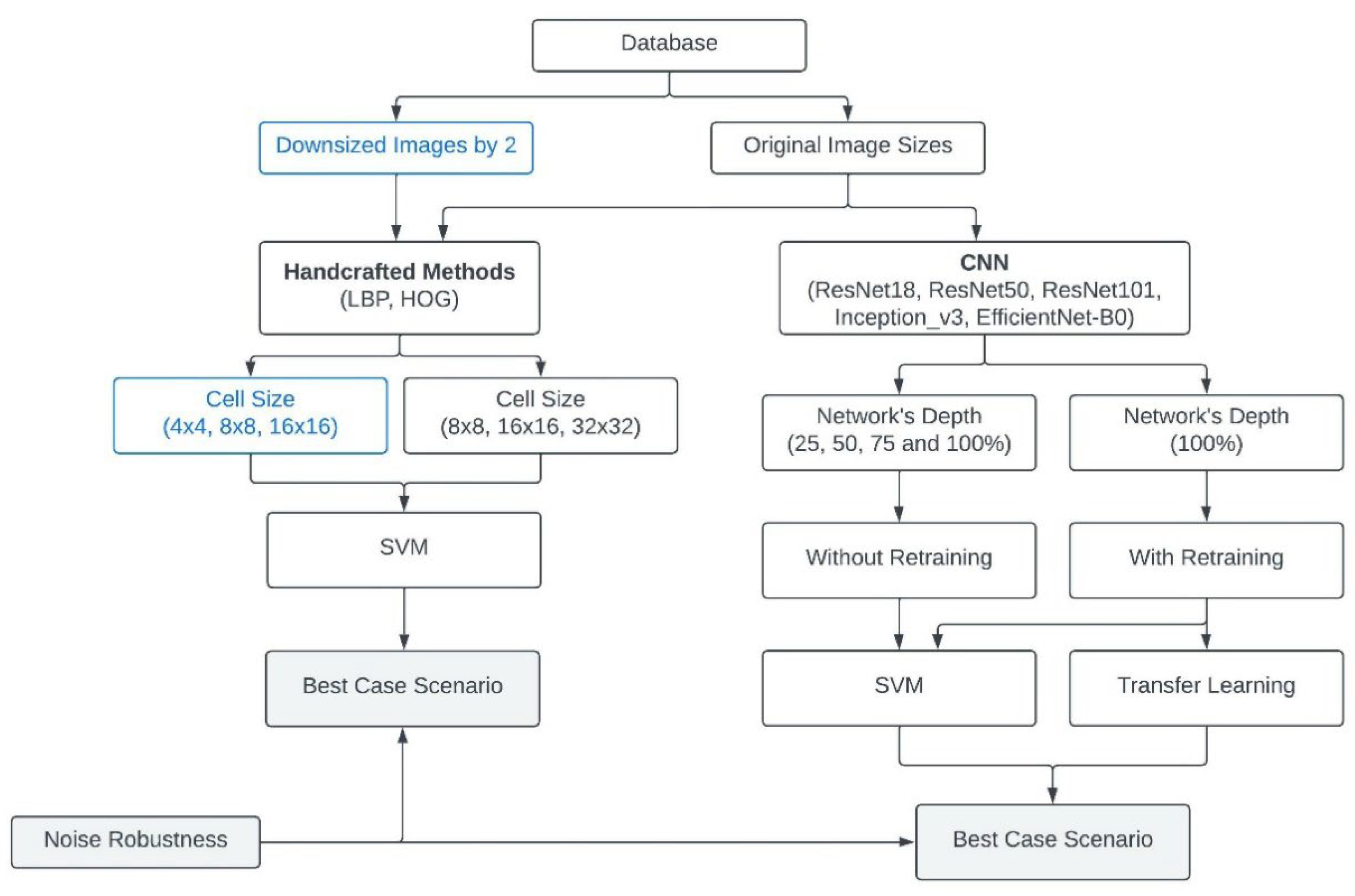
3. Materials and Methods

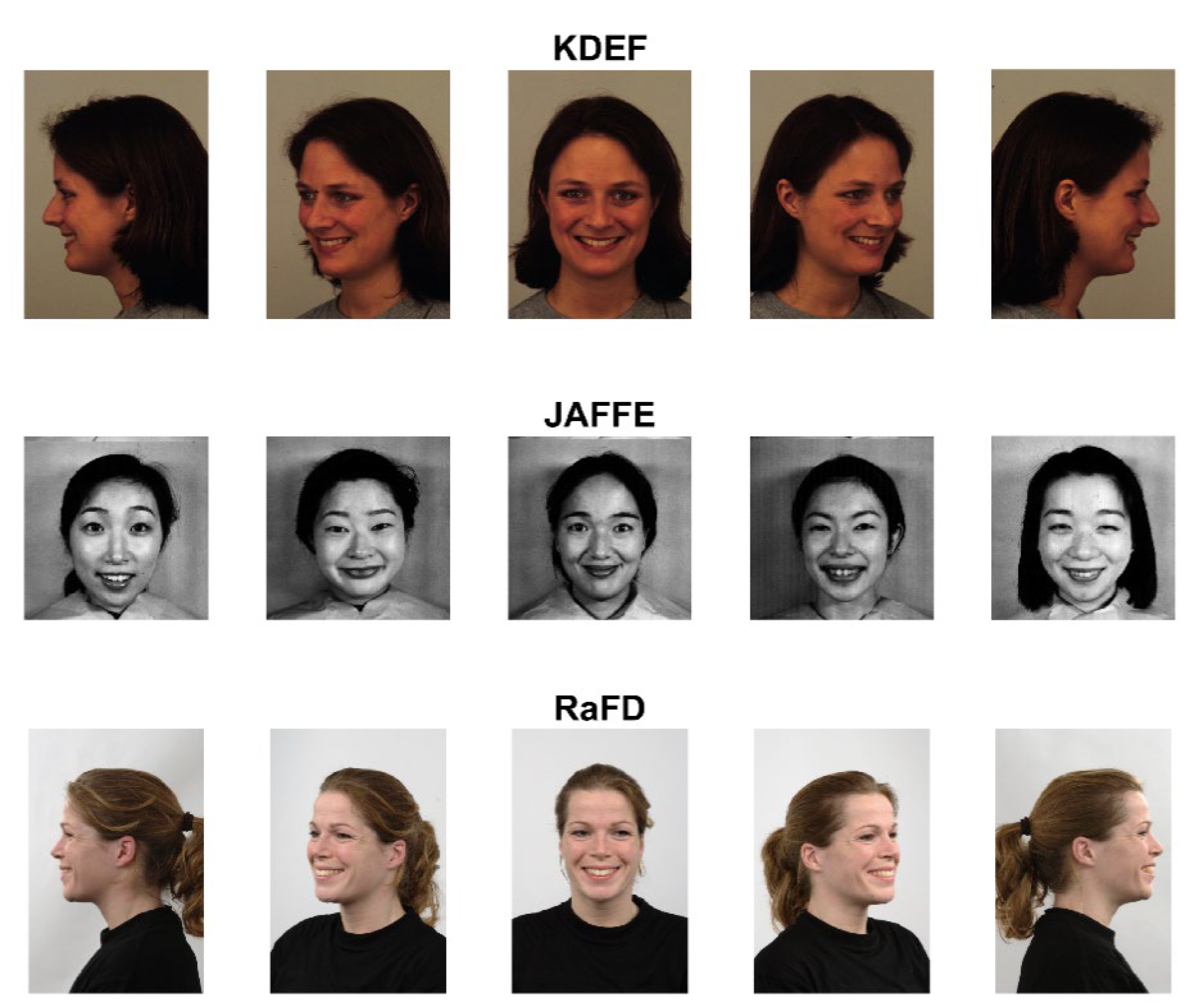
3.1. Databases Selection and Description

The three publicly available databases used include photos collected under controlled shooting conditions where the individuals posed with specific facial expressions. These are:

• KDEF consists of 4900 images divided equally into seven facial emotions viewed from five shooting angles. The participants are males and females in equal parts, between the ages of 20 and 30, who do not wear glasses and jewelry and do not have a beard or mustache. The images are 567 × 762 pixels with 24-bit color values in jpeg format [31];
• JAFFE consists of 213 frontal faces of 10 females expressing seven different emotions. The images are 256 × 256 pixels 8-bit grayscale in tiff format [32]. This database was employed to examine how the algorithms perform in small sets and low-resolution images;
• RaFD consists of 8040 images divided equally into eight facial emotions viewed from five shooting angles. The individuals are Caucasian adults, both men (30%) and women (28%), Caucasian children, both boys (6%) and girls (9%), and Moroccan Dutch males (27%). The images are 681 × 1024 pixels with 24-bit color values in jpeg format [33].

The KDEF and JAFFE databases contain the same seven facial emotions: anger, disgust, fear, happy, neutral, sad, and surprise, while the Radboud Faces Database has one more class, disgust. The details of each database are shown in

Table 1. Databases number of files, classes, poses, colors, dimensions of images, and format.

Database	Files	Classes	Poses	Color	Pixels (Width × Height)	Format
KDEF	4900	7	5	true color	562 × 762	jpeg
JAFFE	213	7	1	grayscale	256 × 256	tiff
RaFD	8040	8	5	true color	681 × 1024	jpeg

:

The databases differ in terms of (a) number of images, (b) image characteristics (resolution, color depth, format), and (c) the number of classes (for RaFD). RaFD and KDEF have a larger number of images, which supports models’ training, but the classification is challenging due to the different shooting angles. Figure 1 shows a sample depicting happiness from each database.

3.2. Feature Extraction

3.2.1. Handcrafted Feature Extraction Methods

The features are identified with the feature detection algorithms, and their analysis with vector values is performed with feature descriptor algorithms. Due to their widespread use in facial recognition applications [34,35,36], we investigate the LBP and HOG feature descriptor algorithms.

(A)

Local Binary Patterns

LBP encodes the texture information of a grayscale image by comparing the difference in the intensity of each pixel with its neighboring pixels. Initially, the image is converted into grayscale. Then the image is divided into rectangular cells [k × k]. Each pixel $i$ in the cell is compared (in terms of intensity) to the neighboring pixels in a circle centered on the i-pixel and radius $r$. In [15], the neighboring pixels are 8, and the radius is 1. By setting the value of the central pixel as the threshold (ranging from 0 to 255), the adjacent pixels get binary values: those with equal or greater values get a value of 1, and those with lower values get a value of 0. These binary values are converted to decimal by multiplying them with powers of 2 (keeping the same direction) and summing them up. The process is repeated with each pixel belonging to 9 different 3 × 3 cells so it can take $2^8$ different values. The 256-bin histogram of the frequency of values taken by each pixel constitutes the 256-dimensional feature vector.

The fact that some of the binary patterns appear more often than others led to an advanced rotation-invariant version of this algorithm named the uniform pattern version [37]. A pattern is uniform when it has at most two transitions 0→1 or 1→0. The histogram, in this case, has one bin for every uniform pattern and one bin for all the non-uniform patterns. The bins are equal to $P\left(P-1\right)+3$, where $P$ is the number of the neighboring pixels. For 8 neighboring pixels, the $2^8=256$-dimension histogram is transformed to a 59-dimensional histogram leading to a 77% reduction in feature size. For an $\left[M\times N\right]$ image, the feature size is given by (1):

$$Feature Siz{e}_{LBP}=\left[floor\left(\raisebox{1ex}{$M$}\!\left/ \!\raisebox{-1ex}{$k$}\right.\right)\times floor\left(\raisebox{1ex}{$N$}\!\left/ \!\raisebox{-1ex}{$k$}\right.\right)\right]\times \left[P\left(P-1\right)+3\right]$$

(1)

(B)

Histogram of Oriented Gradients

HOG technique describes the edges and corners of an object through the distribution of local intensity gradients. For an $\left[M\times N\right]$ image, the gradients of each pixel in the polar form are calculated. These values create the corresponding magnitude and angle matrices with the same dimensions. These matrices are divided into rectangular cells $\left[k\times k\right]$. For all $k^2$ values, a 9-point histogram is calculated, with each point having a width of 20 degrees, ranging from 0 to 160 degrees. The positions in the histogram are selected based on the angle of the gradient, and the values in each bin are derived from the percentage of the corresponding magnitude. These 9-point histograms are grouped into blocks of four $\left(2\times 2\right)$, creating a feature vector 36. The grouping is performed with overlapping of k pixels. So, the size of the feature is given by (2):

$$FeatureSiz{e}_{HOG}=\left[floor\left(\frac{M}{k}-1\right)\times floor\left(\frac{N}{k}-1\right)\right]\times 36$$

(2)

3.2.2. CNN-Based Features

Neural networks generally consist of the input layer, multiple hidden layers, and the output/classification layer. The hidden layers are of three types, the convolutional, the pooling, and the fully connected layers. In the first, as its name implies, the mathematical operation of the convolution between the pixel values and the kernel takes place. After the filter has scanned the entire image, the feature or activation map is created. The pooling layer also scans the whole image, and as the filter has no weights, it gives the maximum or the average value leading to dimensionality reduction. Finally, the fully connected layer performs the classification based on the features extracted from the previous layers. The first hidden layer detects elementary elements of the image, such as edges, which are fed to the next layer that detects more complex elements, such as texture. This process continues with the deeper layer detecting the higher-level features.

Many architectures and techniques have been developed in the last decades resulting in the development of many CNNs. In this research, we choose to employ the CNNs that have applied different methods to improve the classification accuracy; the ResNet architecture, the inception architecture, and the efficient architecture. Specifically, we employ three networks from the ResNet family, namely ResNet18, ResNet50, and ResNet101, to investigate whether network depth affects classification accuracy. In addition, we use Inception_v3 and EfficientNet-B0. We chose these three architectures because they rely on three different tactics to improve classification accuracy. All selected CNNs have a depth of up to about 100 layers and less than 45 million parameters.

• ResNets

The idea behind the development of the Residual Networks family architecture comes from the intuition that the more layers added to a network, the more complex the problems it can solve and the better accuracy it will achieve, which has been refuted. As the depth of the CNNs increases by adding layers, the problem of vanishing/exploding the gradient occurs, resulting in the saturation of the performance first and then its degradation [38]. The ResNet architecture is based on shortcut connections with identity mapping. The output of the shortcut is added to the output of the stacked layers so that if any layer degrades the accuracy, it will be omitted. The CNNs of this family of architecture that are employed in this study are ResNet18, ResNet50, and ResNet101, with the number indicating the corresponding depth of layers.

• Inception_v3

The fact that the object of interest may occupy an arbitrary part of the image led to the Inception architecture. In Inception_v1, filters of different kernel sizes (1 × 1, 3 × 3, and 5 × 5) are applied in the same layer, and their outputs are concatenated into a single output (inception module), forming a network that is wider rather than deeper. Various improvement techniques were applied (such as factorization of 5 × 5 convolution into two 3 × 3 convolutions and the usage of an auxiliary classifier) and led to the advanced version of Inception_v2. The Inception_v3 is a 48 layers-deep network in which, in addition to the techniques of Inception_v2, it applies the factorization of 7 × 7 convolution into three 3 × 3 asymmetric convolutions the batch normalization in the auxiliary classifiers, and the label-smoothing regularization [39].

• EfficientNet

The intuition that the higher the resolution of an image, the greater the depth and the width of the network should be so that the larger receptive fields can detect features of more pixels led to the implementation of EfficientNets. In the architecture of EfficientNets, instead of extending one of the dimensions of the networks (depth, width, or resolution), the technique applied is the uniform scaling of all three dimensions with a set of fixed scaling coefficients, the compound scaling method. The EfficientNet-Β0, chosen in this study, has a depth of 82 layers, which is comparable to the other CNNs of this study [40].

3.3. Model Classifier

Supervised machine learning includes two categories: traditional (i.e., non-CNN) classification algorithms and neural networks. Traditional classification algorithms such as support vector machines (SVM), linear discriminant analysis (LDA), k-nearest neighbors (kNN), Naive Bayes, and many more have been widely used for years and have been compared in terms of their performance in various classification applications [41,42]. In this research, classification accuracy was initially tested with four different algorithms, SVM, LDA, kNN, and random forest, using various combinations of depths and neural networks, and it appeared that all yielded similar results, with SVM being slightly superior to the others (+2% approximately). As a result, SVM with the “one-vs-one” technique has been selected as the representative of the traditional classifiers [43].

4. Scenarios

The workflow of this research is depicted in Figure 2. Each of the databases has been split into the training set containing the 80% of the files and the test set containing the rest 20%. Following, the features are extracted with two methods: (A) handcrafted feature extraction and (B) CNN-based extraction.

For the handcrafted feature extraction, we used the feature descriptors LBP and HOG with the images of the databases with their original dimensions and downsized by two. During the scenarios, maximum accuracy has been achieved with different feature sizes. As the feature size is based on the image resolution, we have investigated the existence of an analogy (ratio) between the image and the feature sizes. To this end, we have downsized by two and by four to verify this ratio.

We apply three cell sizes to the images with their original sizes: $8\times 8, 16\times 16$, and $32\times 32$. To the images downsized by two, we apply cell sizes that produce features of the same size as the original sizes, i.e., $4\times 4, 8\times 8,$ and $16\times 16$. For each combination of image size, descriptor, and cell size, the extracted features feed an SVM classifier to determine the best combination in terms of classification accuracy for each database. We also apply two types of noise, Gaussian and salt and pepper noises imposed on the test set files, in the best combination to investigate the effect on the classification accuracy.

In the CNN-based feature extraction, we use two techniques: the CNNs (ResNet18, ResNet50, ResNet101, Inception_v3, and EfficientNet-B0) as trained on ImageNet (http://www.image-net.org/, accessed on 1 February 2022) and the CNN retrained in the new data. For the originally trained CNN, feature extraction takes place from four different depth levels, i.e., 25%, 50%, 75%, and 100% of its depth, and feeds the SVM classifier. For retrained CNNs, the features are extracted from the last layer (as the intermediate depths did not lead to improved results in terms of classification accuracy and computational time). The extracted features feed the SVM classifier and the CNN’s fully connected layer (transfer learning). No downsizing of the images has been used as the images are resized according to the dimensions required by the CNNs. The comparison in terms of classification accuracy gives the best combination. For this combination, we examine the effect of the two types of noise imposed on the test set files.

The algorithms were implemented with Matlab R2022a and were executed on a desktop PC with 32 GB RAM, with Intel Core i7-10700K processor, eight cores up to 3.8 GHz, with the graphic card NVIDIA GeForce RTX 3060.

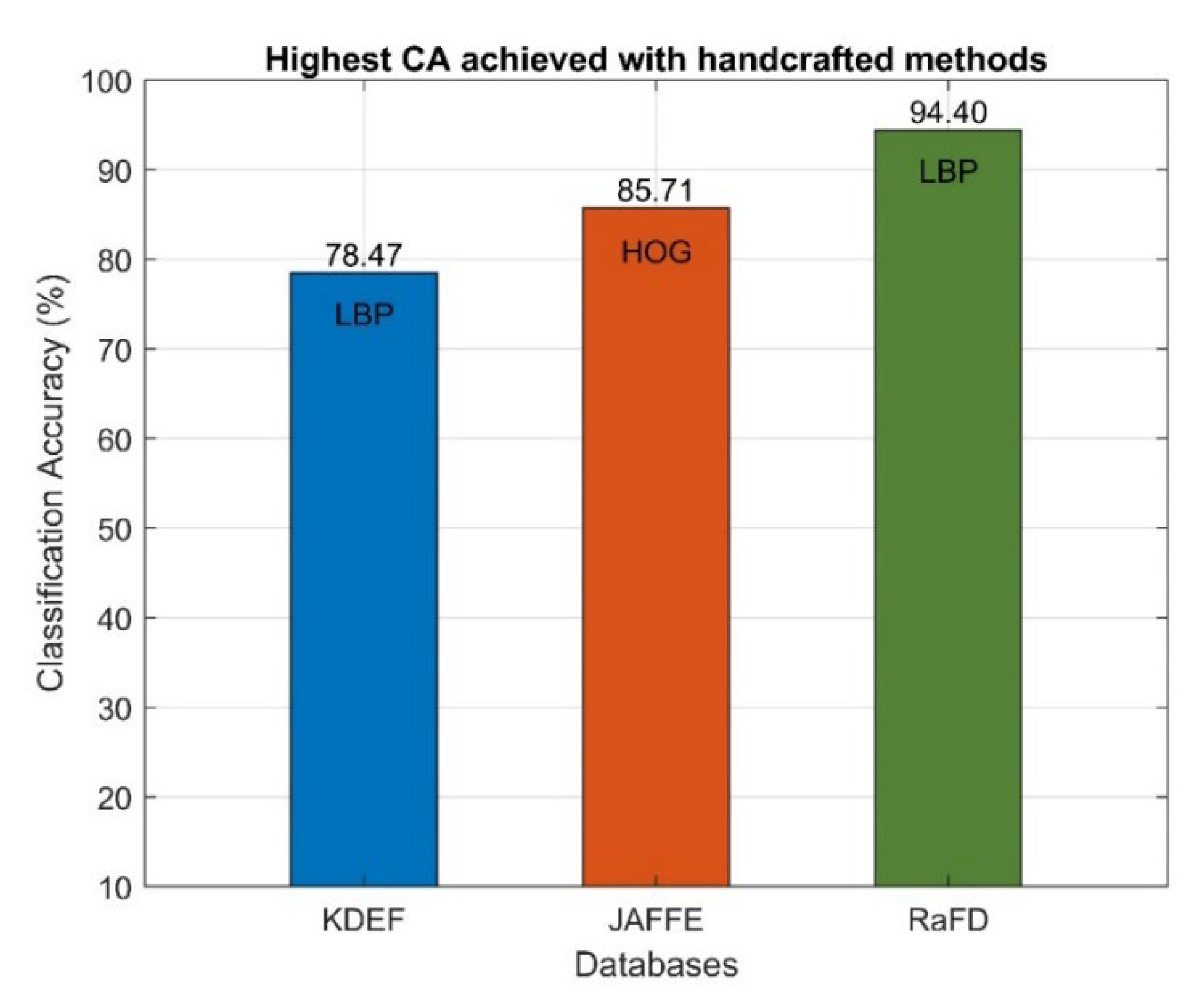
4.1. Extract Features with Handcrafted Methods

In this scenario, we extract the image features with the LBP and HOG methods and feed the SVM classifier. In each method, we investigate the cell size and, therefore, the corresponding feature size, which gives the highest classification accuracy for each database. Both algorithms convert images to grayscale.

First, we export the features from the images at their original sizes. For these dimensions, we use square cells with dimensions of power of two, ranging from 2 × 2 to 64 × 64.

Table 2. Classification accuracy and feature size with LBP method applied to the original image dimensions.

LBP	KDEF		JAFFE		RaFD
Cell Size	Feature Size	CA (%)	Feature Size	CA (%)	Feature Size	CA (%)
8 × 8	392,352	68.84	60,416	78.57	641,920	88.50
16 × 16	97,055	73.65	15,104	76.16	158,592	92.66
32 × 32	23,069	72.32	3776	50.00	39,648	94.40

and

Table 3. Classification accuracy and feature size with HOG method applied to the original image dimensions.

HOG	KDEF		JAFFE		RaFD
Cell Size	Feature Size	CA (%)	Feature Size	CA (%)	Feature Size	CA (%)
8 × 8	233,496	55.57	34,596	80.95	384,048	69.84
16 × 16	56,304	59.65	8100	80.95	92,988	74.63
32 × 32	12,672	56.49	1764	83.33	22,320	76.12

show the results for the cell sizes $8\times 8, 16\times 16$, and $32\times 32$ since the results for cell sizes smaller or larger are inferior. The feature size in both cases results from Formulas (1) and (2), respectively.

For KDEF and RaFD, the two methods give the maximum classification accuracy for the same cell size ($16\times 16$ for KDEF and $32\times 32$ for RaFD). The cell size should give sufficient information with the smallest possible size of a feature vector. However, the texture information method (LPB) yields significantly higher success rates, namely by 14% and 18% for KDEF and RaFD, respectively, compared to the HOG method. JAFFE is an exception to these observations by showing slightly better classification accuracy with HOG features. While both methods use the gradient of the intensity (magnitude and direction) as information around each pixel, the LBP method uses the eight neighboring pixels to detect local patterns, while the HOG method uses one direction for each pixel. This difference makes the LBP method more efficient on the databases with multiple face angles (KDEF and RaFD), while the HOG method on the database with frontal pose images only (JAFFE).

We then divide the dimensions of the image by two, keeping the original aspect ratio to check the role of the resolution in classification accuracy and the correlation between cell size and image dimensions. According to Formulas (1) and (2), when the dimensions of the images are subdivided, the same feature size is obtained for also subdivided cell size, i.e., the size of the feature with the original dimensions of the image for cell size, e.g., $8\times 8$ is equal to that obtained for an image downsized by two for a cell size of $4\times 4$. Therefore, to include the feature with the size that results with cell $8\times 8$, when we subdivide the dimensions of the images, we include the cell size $4\times 4$ and omit the cell size $32\times 32$.

Table 4. Classification accuracy with LBP and HOG methods applied on the images downsized by two.

	KDEF		JAFFE		RaFD
Cell Size	LBP	HOG	LBP	HOG	LBP	HOG
4 × 4	70.07%	59.65%	78.57%	84.21%	85.76%	73.82%
8 × 8	78.47%	69.92%	77.57%	84.71%	92.16%	77.67%
16 × 16	76.20%	61.08%	76.19%	85.71%	94.40%	78.30%

contains classification accuracy results for both methods for downsized by two images of the databases.

The reduction in the images by two positively affects the classification accuracy for KDEF images; it is increased by 6.3% with the LBP method and by 3.3% with the HOG method on average. The same is true for the JAFFE, with a corresponding improvement of 3.1% and 9.5%. Reducing the images by two seems to increase the classification accuracy by 3.1% on average only with the HOG method for the RaFD images, while with the LBP method, we have a reduction in the classification accuracy by 1.1% on average.

The same results were also examined, with the images downsized by four. The classification accuracy, in this case, appeared to be about 2% lower than in the case of downsizing by two, so they are omitted. The observations from Table 1 and Table 2 compared to Table 3 are:

• LBP technique gives significantly improved classification accuracy compared to HOG in all databases, except for the JAFFE database;
• The highest classification accuracy for each technique and database is achieved with the same feature size;
• The downsizing of the images and cells (so that the feature is the same size) improves the classification accuracy up to downsizing by two for all databases. Specifically, the image reduction by a factor of two resulted in improved classification results with the HOG method for all databases. The results are improved only for KDEF and JAFFE databases with the LBP method.

Figure 3 shows the highest classification accuracy achieved for each database with the techniques applied so far. In every case, the images are downsized by two. LBP method proved to be more efficient for KDEF and RaFD databases, while the HOG method for the straight pose images of JAFFE. For KDEF, the optimal cell size is $8\times 8$ and for the JAFFE and RaFD databases is $16\times 16$.

4.2. Extract Features with CNNs

The same image files are used in the training and testing phases in order to compare the methods.

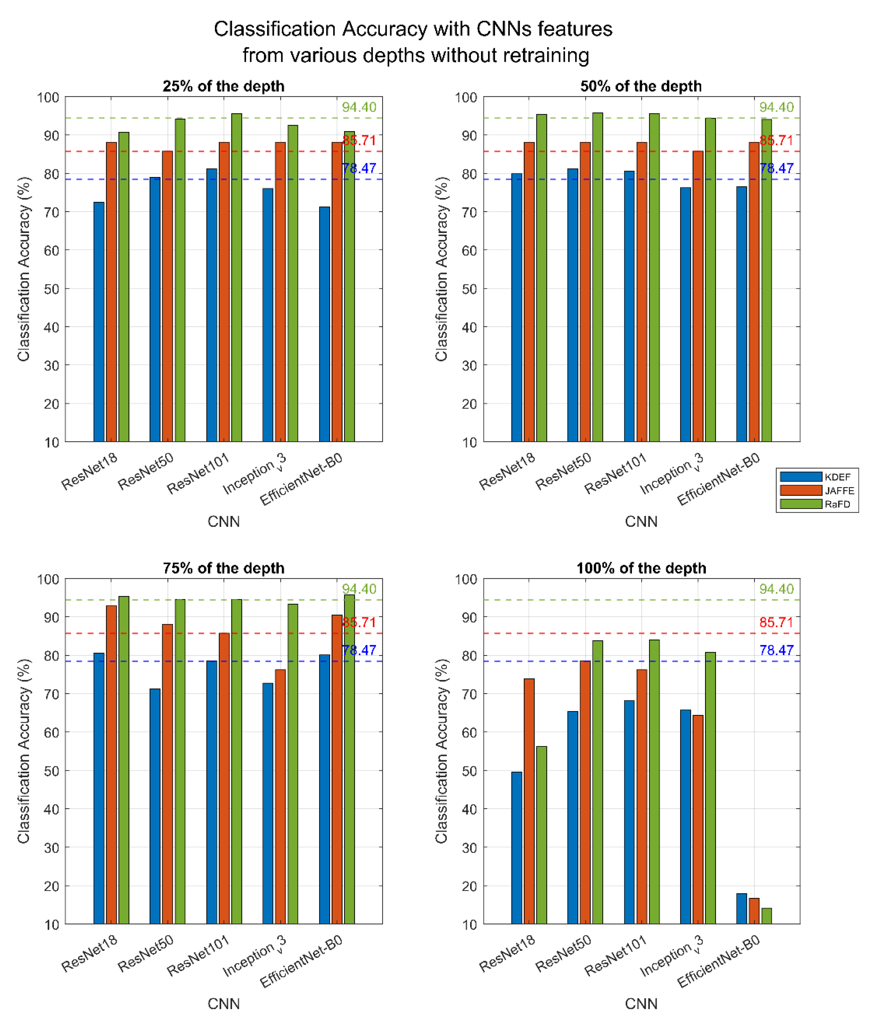
4.2.1. Extract Features without Retraining

Depending on the depth of the layer, the CNNs extract features of different sizes and spatial resolution. We extract features from four different depths of the CNNs, specifically from 25%, 50%, 75%, and 100% of their depth, to identify whether the features extracted from shallower levels are more appropriate than from the output layer.

Figure 4 depicts the results of the classification accuracy per set (blue bar for KDEF, red bar for JAFFE, and green bar for RaFD), per network, and per depth. Extracting features from the last and deepest layer of networks (i.e., from 100% of the depth) leads to the worst results in terms of classification accuracy, with success levels being much lower than those of the handcrafted methods. On the contrary, at 25%, 50%, and 75% of the depth of the networks, the classification accuracy reaches or exceeds the classification accuracy of the handcrafted methods depending on the network used.

At 25% of the depth, the largest in-depth network, ResNet101, performs better than the other networks, giving better results in all three databases. At 50% of the depth, the ResNet family technique performs better, and specifically, ResNet50 gives similar results to those of ResNet101 at 25%, which was to be expected since the difference in the percentage of depth combined with the total depth of the networks gives features of the same size. At 75% of the depth, the results are inferior to the previous ones except for the JAFFE dataset, for which we have the highest performance with ResNet18.

Table 5. Highest classification accuracy and the corresponding total time per method and database.

	Handcrafted Methods			CNNs
Database	CA (%)	Technique	Time (s)	CA (%)	CNN and Depth	Time (s)
KDEF	78.47	(LPB 8 × 8)	1623	81.21	(ResNet50, 50% depth)	1214
JAFFE	85.71	(HOG 16 × 16)	5	92.86	(ResNet18, 75% depth)	55
RaFD	94.40	(LPB 16 × 16)	3746	95.71	(ResNet50, 50% depth)	2988

summarizes the highest classification accuracy per method and the corresponding computation time taken by the algorithms to extract the features and classify the test set. For the cases where we had the same classification percentage with different networks and depths, the selection was made based on the shortest time for exporting results.

Up to this point, extraction of features from ResNet50 without retraining in the new databases from 50% of its depth performs better in comparison with the handcrafted methods in terms of execution time and classification accuracy for the KDEF and RaFD databases. For the JAFFE database, classification accuracy is also significantly improved, with a slight increase in the execution time required by the ResNet18 at 75% of its depth.

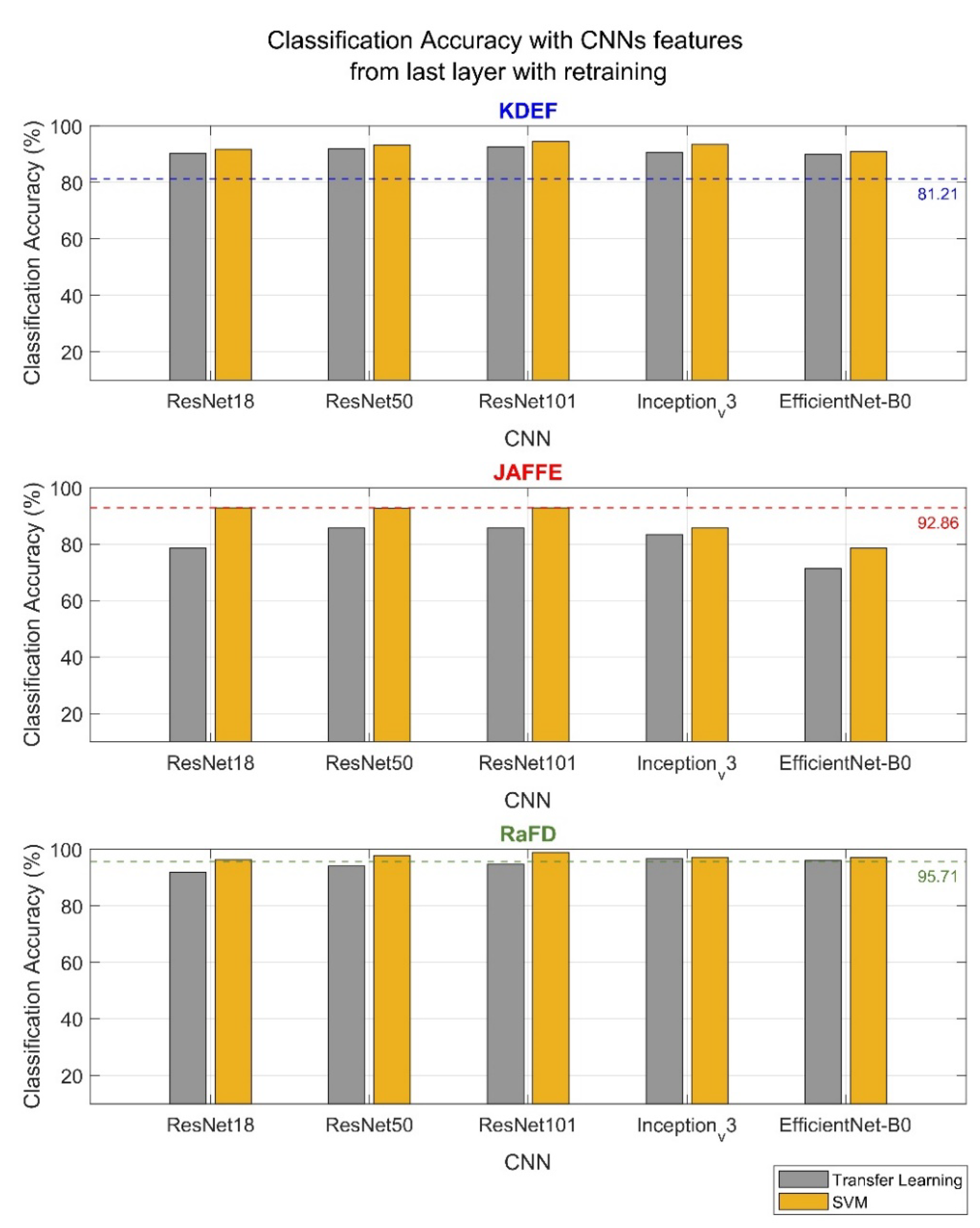
4.2.2. Extract Features with Retrained CNNs

The selection of CNN retraining hyper-parameters values can affect classification accuracy. These hyper-parameters relate to calculating the weights to minimize the loss function by taking corrective steps using back-propagation. The training set is divided by the mini batch size. This quotient is the number of iterations processed by the model to calculate the prediction error and update the weights accordingly. The validation set is used during training to check the intermediate values and make the corresponding corrective steps (learning rate) to select the appropriate weights. An epoch is a complete pass through the entire training set. Validation patience is the number of iterations allowed without an increase in validation accuracy. We consider the work in [44] and set the following values:

• Optimizer is set to the stochastic gradient descent with momentum (SGDM) algorithm to minimize the loss function. In [45], SGDM appears to converge slower but generalizes better than the adaptive moment estimation (Adam) algorithm;
• The learning rate is equal to 0.001, meaning that small correction steps occur in each iteration;
• Since the JAFFE dataset is relatively small (213 images), the mini batch size was set equal to 10, so there is a sufficient number of iterations for weight calculation. The maximum number of epochs was set to 15 so that in combination with;
• The validation patience was set to 2 to check the intermediate values of epochs that are sufficient for retraining. Especially for JAFFE, we did not apply the hyper-parameter of validation patience as it is a small set, and we let the training be performed for all 15 epochs.

Furthermore, we applied additional augmentation operations, including reflections, scaling, and translations, to avoid overfitting.

After retraining the CNNs, the classification of the images in the test set is performed in two ways:

(A)

By extracting the image features from the last (deepest) layer and feeding an SVM classifier with them. In this way, we examine the features in terms of their classification quality before and after retraining.

(B)

By transfer learning. That is, after the fine-tuning of the last layers of each network and the replacement of the outputs with the classes of each database, the classification is performed by the network itself. This way, we compare the classifiers, i.e., SVM and CNNs.

The new results are shown in Figure 5. The dashed lines mark the previous maximum levels of classification accuracy achieved from CNNs without retraining.

The observations include:

• Regarding features, retraining makes sense in sets with numerous files. Especially in KDEF, we observe a significant increase in classification accuracy, while in RaFD, which was already high, it increased slightly. For JAFFE, a small database, we see that network retraining is of no benefit as only the ResNets reach the previous maximum (with SVM);
• Regarding networks and their respective architectures and methods, ResNets deliver higher classification rates, and the deeper the network, the higher the classification accuracy. The Inception_v3 technique follows with results similar to those of ResNet50 for the databases of KDEF and RaFD. Last, the EfficientNet-B0 is performing well only with the most extensive database RaFD, whereas the smallest database, JAFFE, remarks the lowest classification accuracy of all networks;
• As for the classifiers, in all cases, the SVM gives better results than the inbuilt classifier of the CNN.

The computational time required for retraining is depicted in

Table 6. Total time needed (in seconds) for retraining with 80% of the files and extracting results in 20% of the files for all databases.

Database	Total Time (s)
	ResNet18	ResNet50	ResNet101	Inception_v3	EfficientNet-B0
KDEF	2953	6642	8802	6764	19,808
JAFFE	131	327	683	638	1031
RaFD	3604	10,030	22,347	13,014	32,897

.

EfficientNet-B0, in addition to the similar or lower results in classification accuracy, also requires the longest total time. ResNet101 follows with the longest time required, which is expected given that it is also the largest of the networks. A comparison of ResNet50 and Inception_v3 indicates that these two networks are comparable in terms of computational time. Finally, the smaller ResNet18 network requires the shortest time, while its classification accuracy results are close to those of ResNet50 and Inception_v3. Overall, the choice of the network should be made among one of the ResNet architectures, with ResNet50 being the middle ground.

After the retraining of the networks, the maximum classification accuracy has been:

• For the KDEF database, the classification accuracy reached 94.59% with ReseNet101 (an improvement of 13.4%). ResNet50 and Inception_v3 also marked a significant improvement in the classification rate, by 12.1% and 12.3%, respectively, in less time;
• For the JAFFE database, the retraining of the networks did not lead to higher results. The classification rate reached the previous level of 92.86% but with the increased time required for the retraining process;
• For the RaFD database, classification accuracy was increased by 3.17%, reaching 98.88%, with ResNet101 being the highest (in terms of classification accuracy) of all networks.

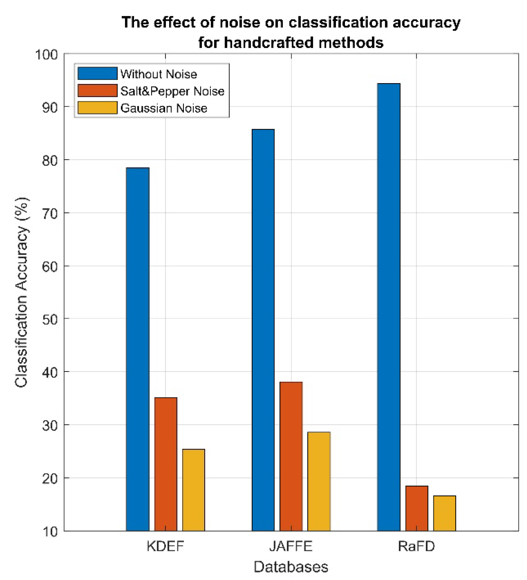
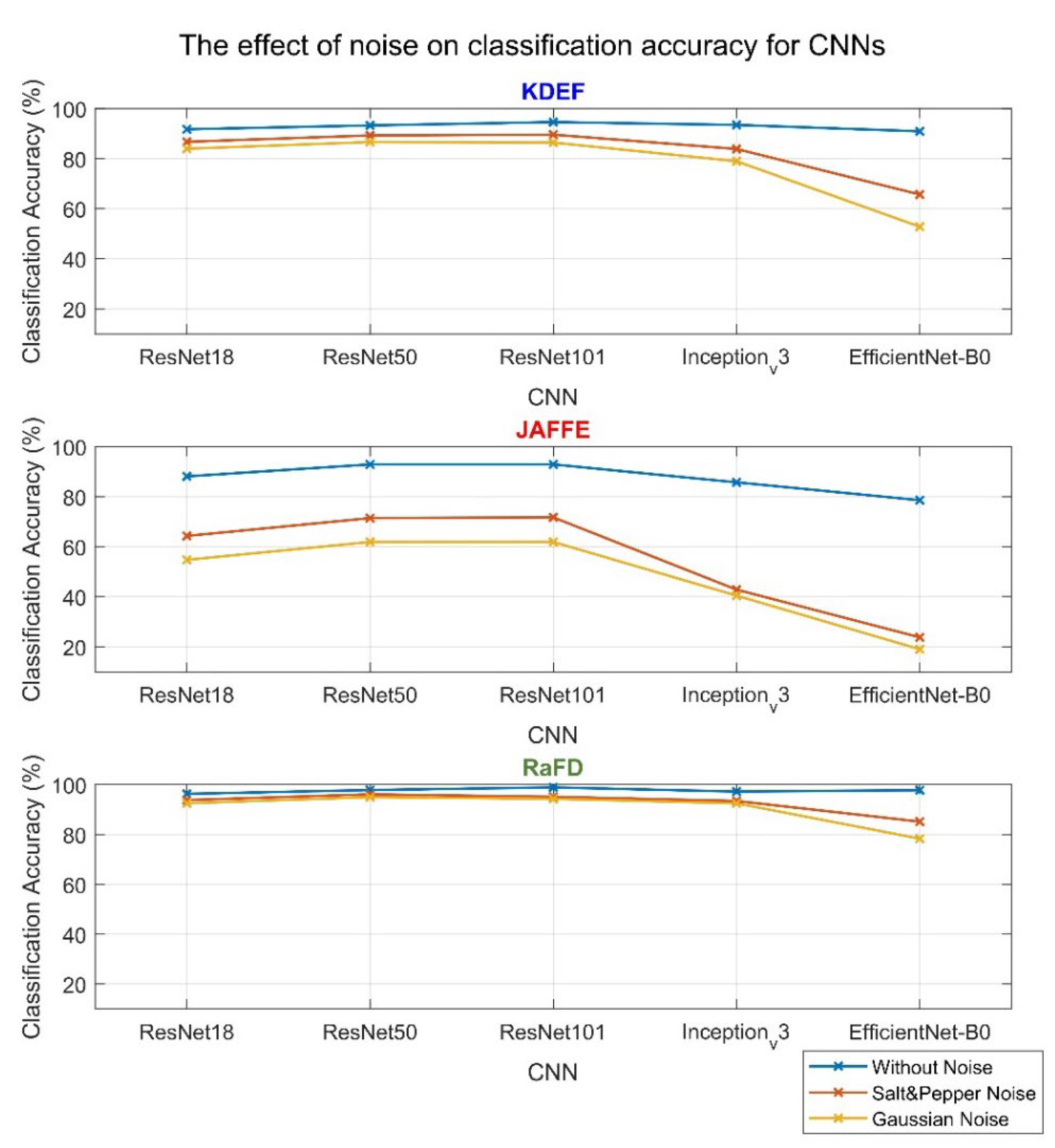
5. Robustness to Noise

Different types of noise can affect the original images. We explore the robustness of the above scenarios to two types of noise. Gaussian noise: occurs during the acquisition of images due to the thermal noise of the sensor and the circuits connected to it. This noise is additive, independent, and independent of each pixel intensity with a normal probability density function and corrupts each pixel [46]. Salt and pepper noise: usually results from bit errors in transmission and image digitizing. In this case of noise, bright (salt) or dark (pepper) pixels are scattered throughout the image [47]. The strength of Gaussian noise is measured with the mean and the variance, while the strength of salt and pepper noise is measured with the rate of the noised pixels [48].

We set these values so that both noises have an average peak signal-to-noise ratio (PSNR) of around 15 dB. Specifically, we examine the effect of noise on the highest success rates achieved with handcrafted and automatic methods. Figure 6 shows the classification performance in corrupted images with the two types of noise resulting from CNNs trained in uncorrupted images, and the classification is performed with the SVM classifier.

The observations that emerge from Figure 7 are:

• All CNNs are more robust (i.e., their classification accuracy is less severely affected by noise) in salt and pepper noise than in Gaussian noise.
• The performance among the networks keeps the same trend in all cases of the databases.
• Low-resolution grayscale JAFFE images appear more affected than KDEF and RaFD color images. In addition, RaFD high-resolution images are less affected by noise.
• The CNNs most affected by corrupted images are EfficientNet-B0 and Inception_v3, with the former being the less robust.
• The most robust network that is the one that, in all cases of the databases, the distance of the results of the classification accuracy between clear and corrupted images is the smallest is ResNet50.

Figure 7. Classification accuracy for each database with handcrafted methods. The blue bar depicts the results on clear images, the red bar on images with salt and pepper noise, and the yellow bar on images with Gaussian noise. The training was performed in clear images.

Figure 7. Classification accuracy for each database with handcrafted methods. The blue bar depicts the results on clear images, the red bar on images with salt and pepper noise, and the yellow bar on images with Gaussian noise. The training was performed in clear images.

Research has been conducted on the robustness of networks to noise. Authors in [49] investigate the performance of deep CNN-based approaches for face recognition applications under several image distortions, including Gaussian and salt and pepper noise. In addition, in [50], it is pointed out that it cannot be predicted in advance how the CNN will behave with noised data. Both the aforementioned studies suggest adding some noise to the training set. We trained the CNNs with noised images, and the classification accuracy resulted between those with clear training and test set and those with a clear training set but a corrupted test set.

Table 7. Percentage deviation of classification accuracy with corrupted test images for each CNN per database.

	ResNet18		ResNet50		ResNet101		Inception_v3		EfficientNet-B0
	Salt and Pepper	Gaussian	Salt and Pepper	Gaussian	Salt and Pepper	Gaussian	Salt and Pepper	Gaussian	Salt and Pepper	Gaussian
KDEF	5.46	8.47	4.28	7.12	5.30	8.65	10.27	15.51	27.75	41.91
JAFFE	27.03	37.84	23.08	33.34	23.08	33.34	49.99	52.77	69.70	75.75
RaFD	2.59	3.94	1.78	2.92	3.83	4.65	3.90	4.86	12.91	19.91

shows the percentage deviations in classification accuracy recorded with corrupted images with the classification accuracy with clean images in each database case and with each CNN case.

A comparison of HOG and LBP robustness toward image distortions, including these two types of noise, have been conducted in [51]. The results show that Gaussian noise has a negative effect on both methods because the edge information is affected, and the sharp gradient change may seem like a fake edge. For the salt and pepper noise, the high or low impulses result in gradients with a larger magnitude, and the direction will point to these noises. This study suggests further investigation on salt and pepper since the two datasets employed gave opposite results.

In our case, the effect of noise on the corresponding higher classification accuracy of the handcrafted models is shown in Figure 7. The results shown are for the respective methods (LBP for KDEF and RaFD databases and HOG for JAFFE database) and the cell sizes that each database showed the highest accuracy classification ($8\times 8$ for KDEF, $16\times 16$ for JAFFE, and RaFD).

Again, Gaussian noise downgrades the classification accuracy more than salt and pepper. Finally, it is noteworthy that both types of noise have the most destructive effects on the richer in terms of image quality and quantity database, i.e., RaFD.

Table 8. Percentage deviation of classification accuracy for each database, with corrupted test files, for the handcrafted methods.

Database	Salt and Pepper Noise	Gaussian Noise
KDEF	55.22	67.72
JAFFE	55.55	66.67
RaFD	80.50	82.48

shows the corresponding deviations in the classification accuracy concerning uncorrupted test images.

6. Conclusions

This research examined the classification accuracy and computation time for facial emotional expressions with a) handcrafted feature extraction methods LBP and HOG and b) CNN-based feature extraction. KDEF, RaFD, and JAFFE databases have been used. The use of neural networks was two-fold. Initially, the features were exported without retraining the networks to the new data, from 25%, 50%, 75%, and 100% of their depths. Extracting features from shallower layers is significantly more efficient if the new images are different from those in which the networks were trained initially (as has been the case in this work). The second use of neural networks was to extract features after retraining them in the new data (transfer learning method).

Table 9. Summary table of classification accuracy and total time results per method and database.

Database	Method	CA (%)	Time (s)
KDEF	Handcrafted: LPB	78.47	1623
	Direct Extraction from the 50% of ResNet50	81.21	1214
	Transfer Learning on ResNet101	94.59	8802
JAFFE	Handcrafted: HOG	85.71	5
	Direct Extraction from the 75% of ResNet18	92.86	55
	Transfer Learning all ResNets	92.86	131,327,683
RaFD	Handcrafted: LPB	94.40	3746
	Direct Extraction from the 50% ResNet50	95.71	2988
	Transfer Learning on ResNet101	98.88	22,347

summarizes the results of the three methods used for the three databases. Regarding the handcrafted methods, LBP gives higher success rates on the high-resolution images of the large databases (KDEF and RaFD), while, on the contrary, HOG on the lower-resolution images of the straight pose of JAFFE. Classification results appear improved by directly extracting features from shallow layers of residual architecture networks. In addition, we observe a reduction in computational time for the large databases compared to the handcrafted methods. Finally, the transfer learning method enhances the classification accuracy for large databases, significantly impacting computational time. The classification accuracy was not improved in JAFFE (as it was a smaller set), with the highest classification rate remaining at 92.86%. The SVM classifier performs better than the inbuilt CNNs classifier.

According to these findings we could build a decision framework to support the appropriate choice based on the specifications of each application. Such a framework is presented in

Table 10. Decision support framework.

Database Type	Criterion	Selection
Small Size Low Quality Straight Poses	High Classification Accuracy	Direct extraction from 75% of the depth of ResNet18
	Short Computational Time	HOG
Medium Size High Quality Multi-angle Images	High Classification Accuracy	Transfer Learning in ResNet101
	Short Computational Time	Direct extraction from 50% of the depth of ResNet50
Large Size High Quality Multi-angle Images	High Classification Accuracy	Transfer Learning in ResNet101
	Short Computational Time	Direct extraction from 50% of the depth of ResNet50

.

Overall, we could say that the handcrafted features implemented for decades do not reach the performance of neural networks. The golden mean between classification performance and computational time is the simplest and fastest method of passing images through CNNs and extracting their features from intermediate layers. If the application requirements need the highest possible classification rate, then a large number of images is necessary to retrain networks. Among the architectures examined, the Residual Networks proved to be the more efficient. The effect of noise is more destructive in handcrafted methods than in CNNs. Of the latter, ResNet50 proved to be the most robust in each case.

7. Future Work

With this research, we could evaluate existing methods of image feature extraction related to the recognition of facial emotions in terms of classification performance with the corresponding compensation in computational time. The images of three well-known publicly available databases were used as provided by their creators and the respective classification rates exceeded 92% in each database case with the retraining of the CNN. Further image preprocessing techniques could improve the individual models’ success rates and computational times. In addition, further investigation of the optimal values of the retraining hyper-parameters could lead to a more complete fine-tuning of the pre-trained models to the new data. Moreover, images in the wild accompanied by postures and gestures could further contribute to the emotion recognition study.

References

1. Picard, R.W. Affective Computing for HCI. HCI 1999, 1, 829–833. [Google Scholar]
2. Sonawane, B.; Sharma, P. Review of automated emotion-based quantification of facial expression in Parkinson’s patients. Vis. Comput. 2021, 37, 1151–1167. [Google Scholar] [CrossRef]
3. Mattavelli, G.; Barvas, E.; Longo, C.; Zappini, F.; Ottaviani, D.; Malaguti, M.C.; Papagno, C. Facial expressions recognition and discrimination in Parkinson’s disease. J. Neuropsychol. 2021, 15, 46–68. [Google Scholar] [CrossRef] [PubMed]
4. Dhuheir, M.; Albaseer, A.; Baccour, E.; Erbad, A.; Abdallah, M.; Hamdi, M. Emotion recognition for healthcare surveillance systems using neural networks: A survey. In Proceedings of the 2021 International Wireless Communications and Mobile Computing (IWCMC), Harbin City, China, 28 June–2 July 2021; IEEE: New York, NY, USA, 2021; pp. 681–687. [Google Scholar]
5. Kaushik, H.; Kumar, T.; Bhalla, K. iSecureHome: A deep fusion framework for surveillance of smart homes using real-time emotion recognition. Appl. Soft Comput. 2022, 122, 108788. [Google Scholar] [CrossRef]
6. Du, G.; Wang, Z.; Gao, B.; Mumtaz, S.; Abualnaja, K.M.; Du, C. A convolution bidirectional long short-term memory neural network for driver emotion recognition. IEEE Trans. Intell. Transp. Syst. 2020, 22, 4570–4578. [Google Scholar] [CrossRef]
7. Ekman, P.; Friesen, W.V. Facial action coding system. Environ. Psychol. Nonverbal Behav. 1978, 1, 97–114. [Google Scholar]
8. Harris, C.; Stephens, M. A Combined Corner and Edge Detector. In Proceedings of the 4th Alvey Vision Conference, Manchester, UK, 31 August–2 September 1988; pp. 147–151. [Google Scholar]
9. Lowe, D.G. Distinctive Image Features from Scale-Invariant Keypoints. Int. J. Comput. Vis. 2004, 60, 91–110. [Google Scholar] [CrossRef]
10. Rosten, E.; Drummond, T. Fusing Points and Lines for High Performance Tracking. In Proceedings of the IEEE International Conference on Computer Vision, Beijing, China, 17–21 October 2005; pp. 1508–1511. [Google Scholar]
11. Bay, H.; Ess, A.; Tuytelaars, T.; Van Gool, L. SURF: Speeded Up Robust Features. Comput. Vis. Image Underst. 2008, 110, 346–359. [Google Scholar] [CrossRef]
12. Calonder, M.; Lepetit, V.; Strecha, C.; Fua, P. BRIEF: Binary Robust Independent Elementary Features. In Proceedings of the 11th European Conference on Computer Vision (ECCV), Heraklion, Crete, Greece, 5–11 September 2010; LNCS Springer: Berlin, Germany, 2010. [Google Scholar]
13. Rublee, E.; Rabaud, V.; Konolige, K.; Bradski, G. ORB: An Efficient Alternative to SIFT or SURF. In Proceedings of the 2011 International Conference on Computer Vision, Barcelona, Spain, 6–13 November 2011; IEEE: New York, NY, USA, 2011; pp. 2564–2571. [Google Scholar]
14. Alcantarilla, P.F.; Bartoli, A.; Davison, A.J. KAZE Features. In Proceedings of the Computer Vision—ECCV, Florence, Italy, 7–13 October 2012; Fitzgibbon, A., Lazebnik, S., Perona, P., Sato, Y., Schmid, C., Eds.; Springer: Berlin/Heidelberg, Germany, 2012; Volume 7577, p. 214. [Google Scholar]
15. Ojala, T.; Pietikäinen, M.; Harwood, D. A comparative study of texture measures with classification based on featured distributions. Pattern Recognit. 1996, 29, 51–59. [Google Scholar] [CrossRef]
16. Dalal, N.; Triggs, B. Histograms of oriented gradients for human detection. In Proceedings of the Computer Society Conference on Computer Vision and Pattern Recognition (CVPR), San Diego, CA, USA, 20–25 June 2005; IEEE: New York, NY, USA, 2005; pp. 886–893. [Google Scholar]
17. Tareen, S.A.K.; Saleem, Z. A comparative analysis of sift, surf, kaze, akaze, orb, and brisk. In Proceedings of the International Conference on Computing, Mathematics and Engineering Technologies (iCoMET), Sukkur, Pakistan, 3–4 March 2018; IEEE: New York, NY, USA, 2018; pp. 1–10. [Google Scholar]
18. Alhindi, T.J.; Kalra, S.; Ng, K.H.; Afrin, A.; Tizhoosh, H.R. Comparing LBP, HOG and deep features for classification of histopathology images. In Proceedings of the International Joint Conference on Neural Networks (IJCNN), Rio de Janeiro, Brazil, 8–13 July 2018; IEEE: New York, NY, USA, 2018; pp. 1–7. [Google Scholar]
19. Alshazly, H.; Linse, C.; Barth, E.; Martinetz, T. Handcrafted versus CNN features for ear recognition. Symmetry 2019, 11, 1493. [Google Scholar] [CrossRef]
20. Lin, W.; Hasenstab, K.; Moura Cunha, G.; Schwartzman, A. Comparison of handcrafted features and convolutional neural networks for liver MR image adequacy assessment. Sci. Rep. 2020, 10, 20336. [Google Scholar] [CrossRef] [PubMed]
21. Nanni, L.; Ghidoni, S.; Brahnam, S. Handcrafted vs. non-handcrafted features for computer vision classification. Pattern Recognit. 2017, 71, 158–172. [Google Scholar] [CrossRef]
22. Zare, M.R.; Alebiosu, D.O.; Lee, S.L. Comparison of handcrafted features and deep learning in classification of medical X-ray images. In Proceedings of the Fourth International Conference on Information Retrieval and Knowledge Management (CAMP), Le Méridien Kota Kinabalu, Sabah, Malaysia, 26–28 March 2018; IEEE: New York, NY, USA, 2018; pp. 1–5. [Google Scholar]
23. Agarwal, S.; Rattani, A.; Chowdary, C.R. A comparative study on handcrafted features v/s deep features for open-set fingerprint liveness detection. Pattern Recognit. Lett. 2021, 147, 34–40. [Google Scholar] [CrossRef]
24. Abdullah, S.M.S.A.; Ameen, S.Y.A.; Sadeeq, M.A.; Zeebaree, S. Multimodal emotion recognition using deep learning. J. Appl. Sci. Technol. Trends 2021, 2, 52–58. [Google Scholar] [CrossRef]
25. Georgescu, M.I.; Ionescu, R.T.; Popescu, M. Local learning with deep and handcrafted features for facial expression recognition. IEEE Access 2019, 7, 64827–64836. [Google Scholar] [CrossRef]
26. Li, B.; Lima, D. Facial expression recognition via ResNet-50. Int. J. Cogn. Comput. Eng. 2021, 2, 57–64. [Google Scholar] [CrossRef]
27. Zhang, H.; Jolfaei, A.; Alazab, M. A face emotion recognition method using convolutional neural network and image edge computing. IEEE Access 2019, 7, 159081–159089. [Google Scholar] [CrossRef]
28. Ahmed, T.U.; Hossain, S.; Hossain, M.S.; ul Islam, R.; Andersson, K. Facial expression recognition using convolutional neural network with data augmentation. In Proceedings of the Joint 8th International Conference on Informatics, Electronics & Vision (ICIEV) and 3rd International Conference on Imaging, Vision & Pattern Recognition (icIVPR), Spokane, WA, USA, 30 May–2 June 2019; IEEE: New York, NY, USA, 2019; pp. 336–341. [Google Scholar]
29. Zang, H.; Foo, S.Y.; Bernadin, S.; Meyer-Baese, A. Facial Emotion Recognition Using Asymmetric Pyramidal Networks With Gradient Centralization. IEEE Access 2021, 9, 64487–64498. [Google Scholar] [CrossRef]
30. Li, K.; Jin, Y.; Akram, M.W.; Han, R.; Chen, J. Facial expression recognition with convolutional neural networks via a new face cropping and rotation strategy. Vis. Comput. 2020, 36, 391–404. [Google Scholar] [CrossRef]
31. Lundqvist, D.; Flykt, A.; Öhman, A. The Karolinska Directed Emotional Faces—KDEF [CD-ROM]; Department of Clinical Neuroscience, Psychology section, Karolinska Institutet: Stockholm, Sweden, 1998. [Google Scholar]
32. Lyons, M.J.; Kamachi, M.; Gyoba, J. Coding facial expressions with Gabor wavelets. arXiv 2020, arXiv:2009.05938. [Google Scholar]
33. Langner, O.; Dotsch, R.; Bijlstra, G.; Wigboldus, D.H.J.; Hawk, S.T.; van Knippenberg, A. Presentation and validation of the Radboud Faces Database. Cogn. Emot. 2010, 24, 1377–1388. [Google Scholar] [CrossRef]
34. Adouani, A.; Henia, W.M.B.; Lachiri, Z. Comparison of Haar-like, HOG and LBP approaches for face detection in video sequences. In Proceedings of the 16th International Multi-Conference on Systems, Signals & Devices (SSD), Istanbul, Turkey, 21–24 March 2019; IEEE: New York, NY, USA, 2019; pp. 266–271. [Google Scholar]
35. Chen, T.; Gao, T.; Li, S.; Zhang, X.; Cao, J.; Yao, D.; Li, Y. A novel face recognition method based on fusion of LBP and HOG. IET Image Process. 2021, 15, 3559–3572. [Google Scholar] [CrossRef]
36. Sun, M.; Li, D. Smart face identification via improved LBP and HOG features. Internet Technol. Lett. 2021, 4, e229. [Google Scholar] [CrossRef]
37. Ojala, T.; Pietikainen, M.; Maenpaa, T. Multiresolution gray-scale and rotation invariant texture classification with local binary patterns. IEEE Trans. Pattern Anal. Mach. Intell. 2002, 24, 971–987. [Google Scholar] [CrossRef]
38. He, K.; Zhang, X.; Ren, S.; Sun, J. Deep residual learning for image recognition. In Proceedings of the IEEE Conference on Computer Vision and Pattern Recognition (CVPR), Las Vegas, NV, USA, 26 June–1 July 2016; pp. 770–778. [Google Scholar]
39. Szegedy, C.; Vanhoucke, V.; Ioffe, S.; Shlens, J.; Wojna, Z. Rethinking the inception architecture for computer vision. In Proceedings of the IEEE Conference on Computer Vision and Pattern Recognition (CVPR), Las Vegas, NV, USA, 26 June–1 July 2016; pp. 2818–2826. [Google Scholar]
40. Tan, M.; Le, Q. Efficientnet: Rethinking model scaling for convolutional neural networks. In Proceedings of the 36th International Conference on Machine Learning, Long Beach, CA, USA, 9–15 June 2019; PMLR 97; pp. 6105–6114. [Google Scholar]
41. Tsalera, E.; Papadakis, A.; Samarakou, M. Novel principal component analysis-based feature selection mechanism for classroom sound classification. Comput. Intell. 2021, 37, 1827–1843. [Google Scholar] [CrossRef]
42. Thanh Noi, P.; Kappas, M. Comparison of random forest, k-nearest neighbor, and support vector machine classifiers for land cover classification using Sentinel-2 imagery. Sensors 2017, 18, 18. [Google Scholar] [CrossRef]
43. Cortes, C.; Vapnik, V. Support-vector networks. Mach. Learn. 1995, 20, 273–297. [Google Scholar] [CrossRef]
44. Tsalera, E.; Papadakis, A.; Samarakou, M. Comparison of Pre-Trained CNNs for Audio Classification Using Transfer Learning. J. Sens. Actuator Netw. 2021, 10, 72. [Google Scholar] [CrossRef]
45. Zhou, P.; Feng, J.; Ma, C.; Xiong, C.; Hoi, S. Towards theoretically understanding why sgd generalizes better than adam in deep learning. arXiv 2020, arXiv:2010.05627. [Google Scholar]
46. Kumain, S.C.; Singh, M.; Singh, N.; Kumar, K. An efficient Gaussian noise reduction technique for noisy images using optimized filter approach. In Proceedings of the First International Conference on Secure Cyber Computing and Communication (ICSCCC), Jalandhar, India, 15–17 December 2018; IEEE: New York, NY, USA, 2018; pp. 243–248. [Google Scholar]
47. Fu, B.; Zhao, X.; Song, C.; Li, X.; Wang, X. A salt and pepper noise image denoising method based on the generative classification. Multimed. Tools Appl. 2019, 78, 12043–12053. [Google Scholar] [CrossRef]
48. Awad, A. Denoising images corrupted with impulse, Gaussian, or a mixture of impulse and Gaussian noise. Eng. Sci. Technol. Int. J. 2019, 22, 746–753. [Google Scholar] [CrossRef]
49. Karahan, S.; Yildirum, M.K.; Kirtac, K.; Rende, F.S.; Butun, G.; Ekenel, H.K. How image degradations affect deep CNN-based face recognition? In Proceedings of the International Conference of the Biometrics Special Interest Group (BIOSIG), Darmstadt, Germany, 21–23 September 2016; IEEE: New York, NY, USA, 2016; pp. 1–5. [Google Scholar]
50. Ziyadinov, V.; Tereshonok, M. Noise immunity and robustness study of image recognition using a convolutional neural network. Sensors 2022, 22, 1241. [Google Scholar] [CrossRef] [PubMed]
51. Ren, H. A comprehensive study on robustness of HOG and LBP towards image distortions. J. Phys. Conf. Ser. 2019, 1325, 012012. [Google Scholar] [CrossRef]
Figure 1. Sample images from the three databases represent the emotion of happiness. Databases KDEF (https://www.kdef.se/, accessed on 16 February 2022) and RaFD (https://rafd.socsci.ru.nl/RaFD2/RaFD?p=main, accessed on 25 February 2022) have five poses, while JAFFE (https://zenodo.org/record/3451524#.YvCEcehBxPY, accessed on 16 February 2022) has only one (frontal) pose.
Applsci 12 08455 g001
Figure 2. Illustration of the workflow.
Applsci 12 08455 g002
Figure 3. Highest classification accuracy achieved for each database with handcrafted methods.
Applsci 12 08455 g003
Figure 4. Classification accuracy as a function of CNN and depth for each database, without retraining with the SVM classifier. Dashed lines depict the highest accuracy achieved with the previous (handcrafted) methods.
Applsci 12 08455 g004
Figure 5. Classification accuracy after retraining each CNN on the corresponding database. The dashed lines depict the previous (without CNNs retraining) highest results for each database.
Applsci 12 08455 g005
Figure 6. Classification accuracy per CNN for each database, with the test performed in clear images (blue line), in images with salt and pepper noise (red line), and in images with Gaussian noise (yellow line), with SVM classifier. The training was performed in clear images.
Applsci 12 08455 g006