Flexible DEM Model Development and Parameter Calibration for Rape Stem

Abstract

The discrete element method (DEM) is an effective technical tool for simulating the dynamic behavior of granular materials in agricultural engineering. However, most of the agricultural materials, such as rape stems, are flexible bodies, and it is difficult to simulate their elastic-plastic characteristics such as bending and failure using the rigid discrete element model. In this research, a flexible DEM model for rape stems was developed and the related parameters were calibrated. The proposed model consists of sequentially arranged rigid units, which were bonded together by the Hertz–Mindlin bonding contact model in the EDEM. The range of the contact parameters of a rape stem was first determined by bench test. The rape stem repose angle test was carried out as an evaluation indicator for the calibration of the DEM contact parameters. The significant factors affecting the repose angle in the contact parameters were discovered using the Plackett–Burman simulation test, and the optimal combination of these parameters was determined based on the response surface simulation test. The rape stem repose angle simulation result was 26.55° with a relative error of 2.2% for the physical tests. The rape-stem flexible DEM model’s bonding parameters were calibrated based on a three-point bending physical test and a Box–Behnken simulation test. The test results show that a rape stem’s maximum damage force obtained from the constructed model was 16.76 N, and the relative error of the measured values from the physical tests was 3.5%. The flexible DEM model could demonstrate the deformation and fracture of rape stems under an external force and can be used for the simulation of harvesting processes such as cutting, conveying, and threshing.

1. Introduction

Rape is the most important oil crop in China, with about 7.2 × 10⁶ hm² planted year-round, and it is an important source of high-quality vegetable oil, providing about 50% of China’s high-quality edible oil [1]. Rape is mainly harvested with combine harvesters [2,3]. The movement pattern of rape material in the harvester and the mechanical relationship with the working parts of the harvester are key to the operational performance of the rape combine harvester, mainly including the feeding of the header, conveying, threshing, etc. [4,5]. Modeling and simulation of the above process can help optimize the performance and cost-effectiveness of combine harvester devices used in rape cultivation [6,7]. The discrete element method (DEM) is a useful numerical technique for simulating discrete body interactions and has a strong potential for the simulation-based design and performance analysis of the crop-to-machine process.

For the simulative study of the rape-harvesting process, discrete element model construction methods have been widely studied for rapeseed long stems, short stalks, seeds, pod shells, light residues, and other materials [8,9,10,11]. However, the above models, in all the simulations mentioned above, were constructed by a multi-spherical method and could not simulate the deformative behaviors of long stems since all the primitive elements were mutually connected in a rigid way. The mechanical behaviors such as the bending and breaking of rape stems during harvesting are difficult to describe when employing a rigid model.

To address the problem of a simulative analysis of flexible bodies such as crop stems, various models have been proposed. Matthew Schramm constructed a flexible fiber wheat straw DEM model that includes a mega-particle comprising smaller particles and bonded by four beam shaped bonds. The related parameters were calibrated by the three-point bending test and uniaxial compression test of wheat straw. The regression meta-model was established between the particle contact Young’s modulus and the bond Young’s modulus and Poisson’s ratio to predict the Young’s modulus of flexible wheat straw [12]. Fanyi Liu developed a flexible wheat straw model based on the Hertz–Mindlin with bonding model using the discrete element method. A single-factor sensitivity analysis and calibration of the bonding parameters were performed using a three-point bending test. The small difference between the simulated and measured elastic modulus was less than 4.2% [13]. Tom Leblicq developed a segmented wheat stem for a DEM simulation with a number of realistic bending parameters. The effects of plastic deformation and damage could be incorporated into the model. Stem bending measurements showed that the model could predict the force–deformation relationship under different numbers of segments, stem lengths, support distances, and different degrees of plastic deformation [14]. Liao Yitao carried out a bolting-stage rape crop-stalk-chopping model and the parameters were calibrated. A number of spheres were bonded, replacing the whole stalk. The error between the simulation and the physical test value of the bending force until breaking was less than 4. 21% [15].

In this research, a flexible rape stem DEM model was developed based on rigid rape stem units and bonding keys. The basic range of rape stem interaction parameters was tested by the developed test bench. Repose angle physical and simulation experiments were carried out to determine the significant factors and optimal parameter combinations in the collision parameters. Based on the collision parameters, the Hertz–Mindlin with bonding model and its bonding parameters were investigated according to the three-point bending test. The bending behavior of a rape stem was simulated using the developed flexible DEM model and was experimentally verified. The rape-stem flexible DEM model could be used for the simulation of harvesting processes such as cutting, conveying, and threshing.

2. Materials and Methods

2.1. Rape’s Characteristic Material Parameters

The characteristic material parameters for constructing a discrete element model of rape stems mainly include triaxial dimension, density, shear modulus, and Poisson’s ratio. According to the previous studies, the shear modulus and Poisson’s ratio of rape stems were determined as 1.1 × 10⁷ Pa and 0.4, respectively [16,17,18]. Other characteristic material parameters were tested by field sampling. The rape variety in this study was Zheyou 51, collected in June 2022 at the lower reaches of Yangtze River Plains, located in Liyang, Jiangsu province, China (119.4837° E, 31.41538° N). The average planting density, biomass, yield, and height were about 4.34 × 10⁵ plant/hm², 1.25 × 10⁴ kg/hm², 2.3 × 10³ kg/hm², and 1457.0 mm, respectively. The rape stem was stout at the bottom and weak at the top of the plant. The diameter of the main stem was measured at 100.0 mm intervals starting from 50.0 mm above the ground. The average diameter of the stems was 7.1 mm, and the stem density was determined to be 486 kg/m³ by weighing the stem mass and calculating the volume. The material parameters required for the rape stem DEM simulation are shown in the

Table 1. Simulation parameter.

Parameter			Value
Intrinsic parameter	Rape stem	Poisson’s ratio	0.4 a
		Density/kg·m−3	486 b
		Shear modulus/Pa	1.1 × 107 a
	Steel	Poisson’s ratio	0.3 a
		Density/kg·m−3	7850 a
		Shear modulus/Pa	7.9 × 1010 a
Contact parameter	Rape stem–rape stem	Coefficient of restitution (A)	0.322~0.611 c
		Coefficient of static friction (B)	0.381~0.752 c
		Coefficient of rolling friction (C)	0.013~0.032 c
	Rape stem–steel	Coefficient of restitution (D)	0.298~0.623 c
		Coefficient of static friction (E)	0.284~0.730 c
		Coefficient of rolling friction (F)	0.021~0.042 c

Note: ^a indicates that the item is obtained from the literature; ^b indicates that the item is determined by the physical test; ^c indicates that the item is the parameter to be determined.

.

2.2. Rape Stem Contact Parameters Test

The construction of a discrete element model for rape stems requires the determination of contact characteristic parameters between the stem–stem and stem–external materials. In this paper, bench tests were conducted to determine the basic range of rape stem contact parameters, and then the optimal combination of the parameters was determined by simulation tests. The contact parameters include coefficient of restitution, coefficient of static friction, and coefficient of rolling friction. Q235 steel was selected as the contact material since it is commonly used in agricultural machinery.

The test bench composed of Q235 is shown in Figure 1. The material box is a cube without the bottom plate. The material can fall freely after the baffle is pulled out. The horizontal angle of the test plate can be freely adjusted for determining the coefficient of restitution. The coefficient of static friction and coefficient of rolling friction can be determined by adjusting the angle of the base plate. The contact characteristic parameters of the stem-Q235 can be directly determined by this device. When measuring the characteristic collision parameters between stems–stems, the stems were bonded onto the test plate and the base plate in advance.

2.2.1. Coefficient of Restitution

The coefficient of restitution is an important mechanical parameter reflecting the collision characteristics during agricultural machine–rape stem interactions. The coefficient of restitution is defined as the ratio of the normal partial velocity of the center of mass of two objects before and after a collision [19], and is a parameter to measure the restitutive ability of an object after deformation. The test method for the rape stems’ coefficient of restitution is shown in Figure 2.

Before the test, the rape stem was sectioned into 20.0 mm, 30.0 mm, 40.0 mm, and 50.0 mm lengths and placed in the material box. After the baffle plate was pulled, the rape stem started to move in free-fall. The stem velocity when in contact with the test plate is

$$\left\{\begin{array}{l}{h}_1=\frac{1}{2}g{t}_1^2\\ v_1=g{t}_1\end{array}\right.$$

(1)

$$v_1=\sqrt{2g{h}_1}$$

(2)

where h₁ is the vertical distance between the baffle plate and the center of the test plate, m; t₁ is the free fall motion time, s; v₁ is the normal fractional velocity of rape stem before the collision, m/s.

The stem collides with the test plate and then falls on the bottom plate after an oblique throwing motion:

$$\left\{\begin{array}{l}{h}_2=-v_{2y}{t}_2+\frac{1}{2}g{t}_2^2\\ S=v_{2x}{t}_2\\ v_{2x}=v_2\cos \left(90-2\alpha \right)\\ v_{2y}=v_2\sin \left(90-2\alpha \right)\end{array}\right.$$

(3)

$$v_2=\frac{S}{\sin 2\alpha \sqrt{\frac{2\left(h_2+S\cot 2\alpha \right)}{g}}}$$

(4)

where h₂ is the vertical distance between the test plate and the base plate, m; v₂ is the normal fractional velocity of rape stem after the collision, m/s; t₂ is the oblique throwing motion time, s; v_2y is the components of v₂ in the vertical direction, m/s; v_2x is the components of v₂ in the horizontal direction, m/s; α is the angle between the test plate and the horizon, (°); S is the horizontal distance between rape stem-bottom plate contact point and the center of the test plate, m.

According to Equations (2) and (4), the coefficient of restitution’s calculation formula is:

$$c_r=\frac{v_2}{v_1}=\frac{S}{2\sin 2\alpha \sqrt{h_1\left(h_2+S\cot 2\alpha \right)}}$$

(5)

where c_r is the coefficient of restitution’s calculation.

In this research, h₁ = 0.45 m, h₂ = 0.45 m, and α = 45°. The variable that needs to be measured is S. Each length of rape stem was tested 30 times in duplicate. The coefficient of restitution between rape stem–steel and rape stem–rape stem was [0.322, 0.611] and [0.298, 0.623], respectively.

2.2.2. Coefficient of Static Friction

The coefficient of static friction is the ratio of the maximum static frictional force on the object to the normal pressure. The rape stem coefficient of the static friction test method is shown in Figure 3. In the initial state, the rape stems to be tested were placed axially on the horizontal test plate. The test plate was slowly lifted and stopped when the rape stem slipped. The angle θ_s displayed by the angle scale was recorded at this time, and the static friction coefficient was calculated according to Equation (6).

$${\mu }_s=\tan {\theta }_s$$

(6)

where μ_s is the rape stem coefficient of static friction; θ_s is the friction angle, (°).

The rape stems of 20.0 mm, 30.0 mm, 40.0 mm, and 50.0 mm lengths were each replicated 30 times. The coefficient of static friction between rape stem–steel and rape stem–rape stem was obtained as [0.284, 0.730] and [0.381, 0.752], respectively.

2.2.3. Coefficient of Rolling Friction

Rolling friction refers to an object on the surface of another object that possesses non-slip rolling properties or a tendency to roll, where the object in contact with the surface experiences deformation due to rolling hindrance. The rape stem’s coefficient of rolling friction for the test method and the mechanical state of the rape stem are shown in Figure 4. The test plate was placed horizontally and the rape stems to be tested were placed radially on the test plate. The test plate was slowly lifted and stopped when the rape stem rolled on the surface of the test plate.

The stem tends to roll down the slope under the action of gravity. The rolling torque is:

$$M_1=G_{s}r\sin {\theta }_r$$

(7)

where r is rape stem radius, mm; M₁ is rolling torque, N·m; G_s is rape stem gravity, N; θ_r is the angle between base plate and frame, (°).

The rape stem remains stationary under the action of the roll resistance. The rolling resistance torque is:

$$M_2=f_r{G}_s\cos {\theta }_r$$

(8)

where f_r is coefficient of rolling friction; M₂ is the rolling resistance torque, N·m.

In the critical state:

$$\left\{\begin{array}{l}{M}_1=M_2\\ G_{s}r\sin \theta =f_r{G}_s\cos {\theta }_r\end{array}\right.$$

(9)

The coefficient of rolling friction can be calculated as:

$$f_r=r\tan {\theta }_r$$

(10)

The rape stems of 20.0 mm, 30.0 mm, 40.0 mm, and 50.0 mm lengths were each replicated 30 times. The coefficient of rolling friction between rape stem–steel and rape stem–rape stem was obtained as [0.013, 0.032] and [0.021, 0.042], respectively.

2.3. Rape Stem Contact Parameter Calibration

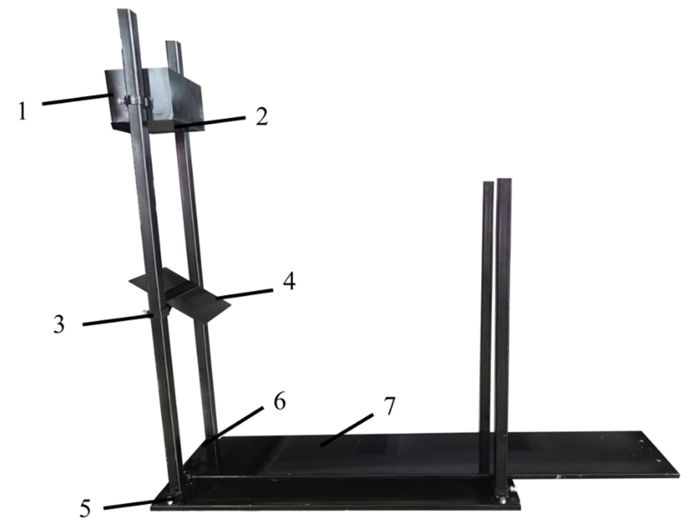
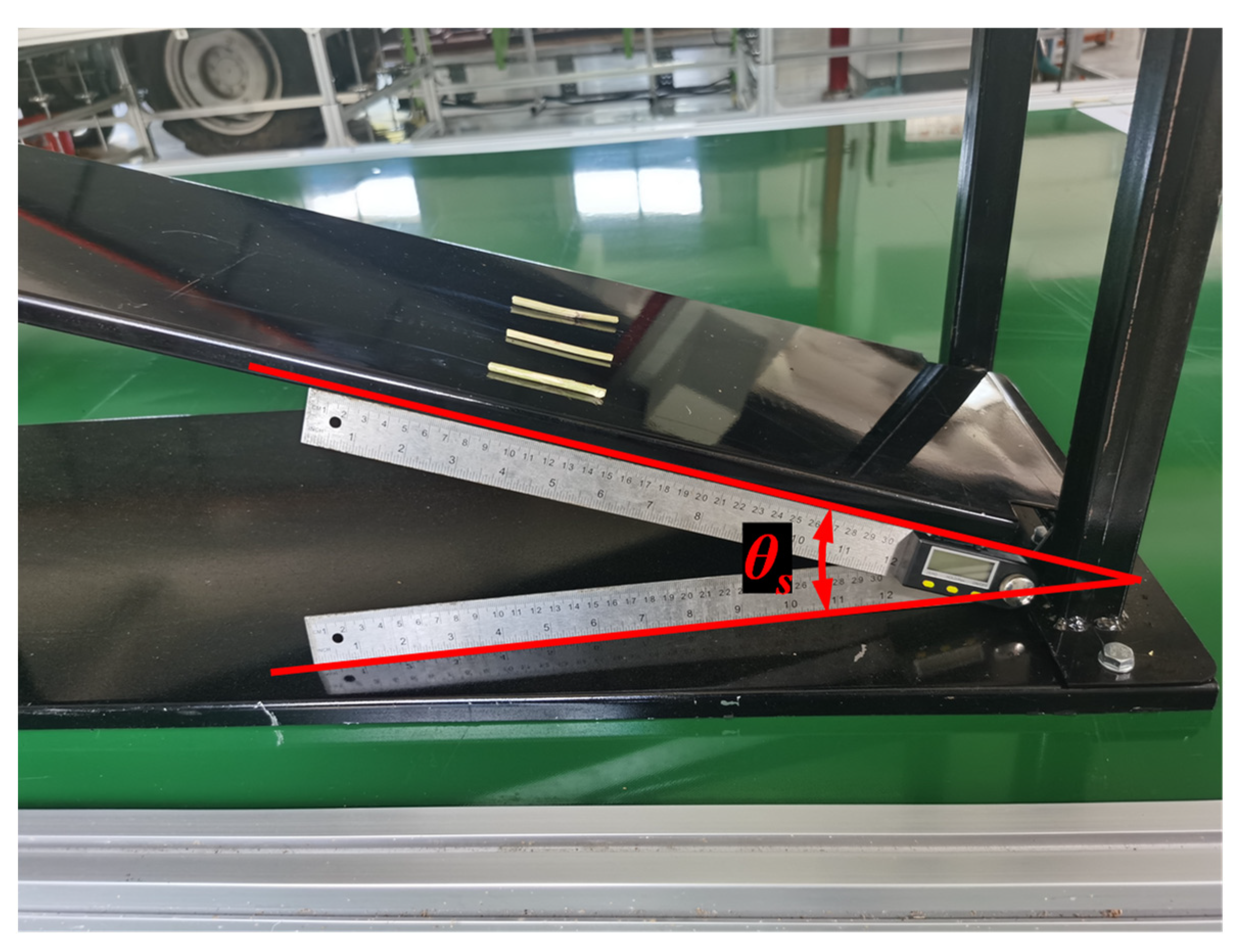
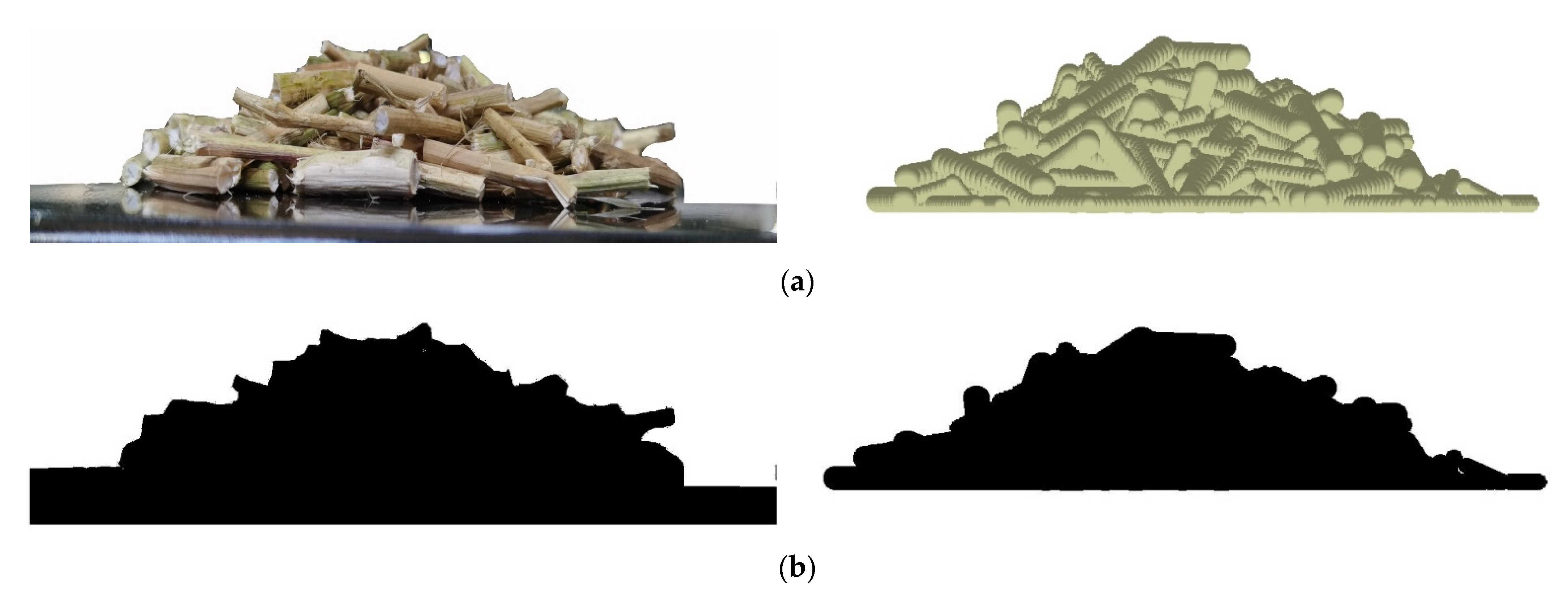
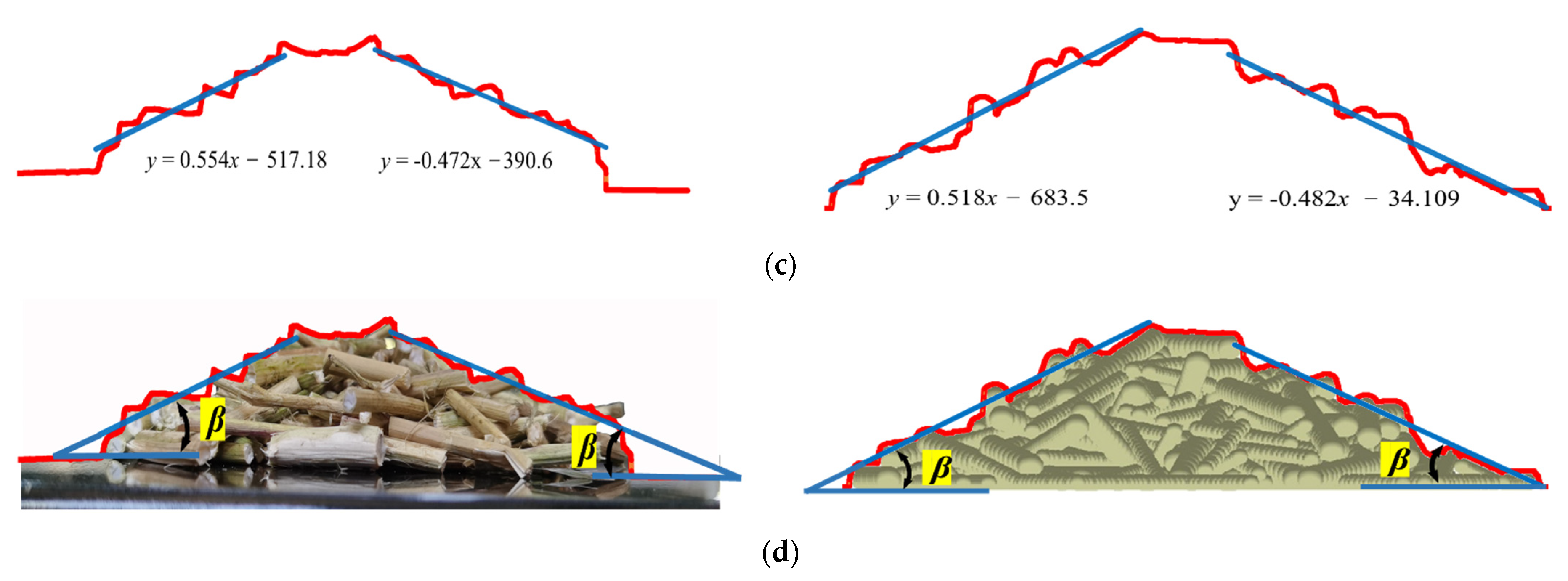
2.3.1. Rape Stem Repose Angle Test

A cone will form when a discrete material is dumped in a plane, and the inner angle made by the cone and the horizontal plane is the repose angle. The angle of repose is a macroscopic parameter characterizing the flow and friction of granular materials and is related to particle density, particle surface area, and particle friction coefficient. Therefore, the repose angle test is often used as the discrete elements parameter calibration for material [20,21]. The cylinder lifting method is a common means to obtain the repose angle [22].

Mixed rape stems with diameters of about 6.0 mm, 7.0 mm, and 8.0 mm were selected for the cylinder lifting repose angle test. Rape stems were prefabricated into 20.0 mm, 30.0 mm, and 40.0 mm lengths, and mixed rape stems with 9 sizes of samples were used in the test. A steel cylinder (with a diameter of 120.0 mm and height of 100.0 mm) was fixed on the universal-material-testing machine and its bottom surface was in contact with the test bench. The rape stems were filled into the steel cylinder until it was full. The steel cylinder was lifted upward at a speed of 0.05 m/s so that the rape stems formed a granule pile, as shown in Figure 5a. After trial, the frontal image of the accumulated stems was captured and binarized. The boundary was extracted by the edge detection method and the linear fitting method was used to calculate the slope of the boundary to obtain the repose angle. The test was repeated 5 times and averaged.

2.3.2. Rape Stem Repose Angle Simulation Model

The rape stems’ repose angle was further studied by DEM. The rape stem discrete element model was built in the DEM software EDEM 2018 (DEM Solutions Limited, Edinburgh, UK). Each rape stem was approximated as a cylinder and filled with spherical particles as shown in Figure 6. To match the repose angle physical test, rape stem models with lengths of 20.0 mm, 30.0 mm, and 40.0 mm and diameters of 6.0 mm, 7.0 m, and 8.0 mm were established. The steel cylinder’s size and lifting speed and rape stem’s quality in the simulation were consistent with the physical test, as shown in Figure 5b.

The Hertz–Mindlin (no slip) model was chosen as the particle model and particle contact model in the EDEM software for rape stems. The simulation time step, environmental gravitational acceleration, and preservation interval were 0.5 × 10⁻⁶ s, 9.8 m·s⁻², and 0.01 s, respectively. The simulation time was 2.0 s to ensure that the rape stems remained stationary and so the repose angle no longer changed. The related contact-mechanical characteristic parameters between the rape stem and the steel are shown in Table 1.

2.3.3. Rape Stem Contact Parameter Calibration Method

Due to the large number of stem contact parameters, the significant parameters affecting the repose angle needed to be screened first. The Plackett–Burman method is a two-level experimental design method whereby the significance of the factors is determined by comparing the difference between the two levels of each factor with the overall difference. In this research, based on the basic parameter range determined by the physical repose angle test, the key simulation model parameters affecting the repose angle were investigated by the Plackett–Burman test. The test was conducted in 14 groups, with 2 groups of central levels for model’s validation. To reduce the influence of random factors such as material generation position and angle on the test results, each group of tests was repeated 5 times and averaged. Contact parameters that significantly affected the repose angle were determined by ANOVA and t-test. Response surface tests were conducted with these significance parameters as variables to determine the optimal combination of parameters for the rape stem contact parameters.

2.4. Calibration of Flexible Discrete Element Parameter for Rape Stem

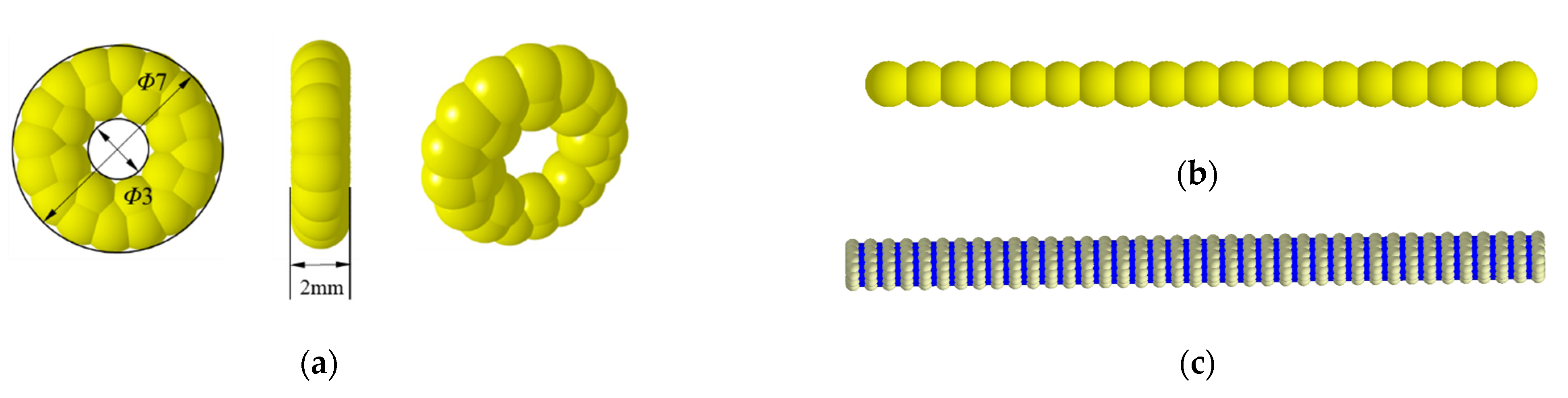
2.4.1. Flexible Discrete Element Model

The position of each spherical unit in the rigid stem model is fixed, so it cannot simulate the deformation behaviors of the stem such as bending and twisting. To address the problem wherein the rape stem is a flexible body and the rigid model cannot accurately express its mechanical characteristics, the rape stem flexible discrete element model (Figure 7) was built based on EDEM API and Hertz–Mindlin with Bonding contact model.

Firstly, a rigid unit for the rape stem flexible model was built through spherical particle filling as shown in Figure 7a. The rape stem was approximated as a hollow structure since the internal spongy structure of the rape stem is loose and of low strength. According to the result of the rape stems’ structure test, the overall diameter of the rigid discrete unit and the internal hollow core diameter were determined to be 7.0 mm and 3.0 mm, respectively. Spherical particles with a diameter of 2.0 mm were used for filling, and each rigid unit contained 24 particles. Secondly, several rigid units were arranged sequentially along their axes through the EDEM software particle factory API. Finally, the rigid units were bonded together (Figure 7c) by the Hertz–Mindlin with bonding contact model to replace the initial rape stem rigid discrete element model (Figure 7b). The rigid units are bonded to each other and able to withstand a certain amount of normal and tangential displacement. The bond will fracture when reaching the critical normal and tangential stresses. Thus, the developed rape stem flexible model can simulate a variety of mechanical behaviors such as tensile, bending, torsion, and fracture behaviors.

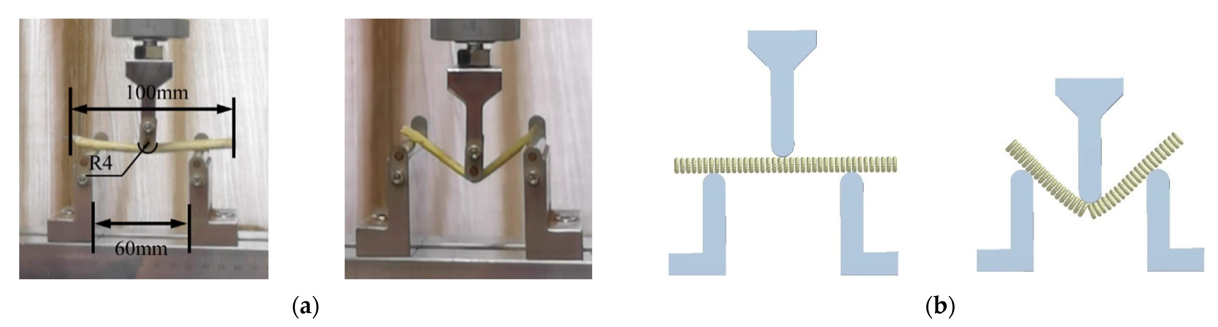
2.4.2. Three-Point Bending Test

The three-point bending test could quantify and comprehend the elastoplastic flexural behavior of crop stalk [23]. In this research, the maximum damage force of the rape stems was obtained by the three-point bending test, which was used to calibrate the bonding parameters of the flexible discrete element model.

The test device is shown in Figure 8a. The loading device was the electronic universal testing machine (utm6503, Suns, Shenzhen, China). The test materials were selected from rape stems with an average diameter of 7.0 mm (with 95% confidence interval lower and upper limits of 6.7 mm and 7.4 mm, respectively). The moisture content of the rape stems was measured to be 51.3%. The distance between the support points on both sides of the sample was 60.0 mm, and the loading speed was 1 mm/s. The support cylinder and loading cylinder radii were 4.0 mm. The rape stem was extruded and deformed under the load until broken, and the maximum bending-damage force was recorded. The test was repeated 5 times and averaged, resulting in a mean maximum damage force of 16.20 N and a coefficient of variation of 4.94%.

2.4.3. Bonding Parameter Calibration

In the Hertz–Mindlin with Bonding contact model, the key parameters include normal stiffness per unit area, shear stiffness per unit area, critical normal stress, critical shear stress, and bonded radius. Referring to the vine materials and existing studies on agricultural material simulation parameters, the critical normal stress and critical shear stress are not significant in the discrete element model of crop stems and can be taken as the values of 45.0 Mpa and 7.0 Mpa, respectively [24,25]. The stiffness per unit area, shear stiffness per unit area, and bonded radius were determined by the Box–Behnken response surface test.

The established discrete element model for rape stems’ flexibility was applied to conduct a three-point bending simulation test. The maximum damage force of the three-point bending test was used as the response value to determine the optimal combination of bonding parameters. The simulation test is shown in Figure 8b. The simulation fixed time step was 5.0 × 10⁻⁷ s and other conditions were consistent with the physical test. The bonding parameter range is shown in

Table 2. Bonding parameter.

Factor	Level
	−1	0	1
Stiffness per unit area (G)/N·m−3	1.0 × 109	5.5 × 109	1.0 × 1010
Shear Stiffness per unit area (H)/N·m−3	1.0 × 108	5.5 × 108	1.0 × 109
Bonded radius (I)/mm	1.0	1.5	2.0

. The effect of bonding parameters and their interaction on stem bending damage was analyzed by ANOVA. The relationship between the bonding parameters and the rape stems’ maximum bending-damage force was modeled to solve the optimal combination of parameters.

3. Results and Discussion

3.1. Contact Parameter

3.1.1. Repose Angle Test

The results of the physical and simulation tests of the rape stems’ repose angle are shown in Figure 9a. The result of the binarization of the stem-piling image is shown in Figure 9b. The discrete rape stems were tapered and stacked on a flat surface, but some of the stems protruded from the tapered boundary. The boundary of the stacked stems was further extracted and linearly fitted as shown in Figure 9c. The rape stem repose angle was obtained as shown in Figure 9d, and the mean value of the rape stem repose angles was 27.15° with a coefficient of variation of 1.27% from five replicate trials. The same algorithm was applied to the simulation results. The simulation results indicate that the established discrete element model can simulate the piling process of the rape stems, and that the DEM contact parameter can be calibrated by the repose angle test.

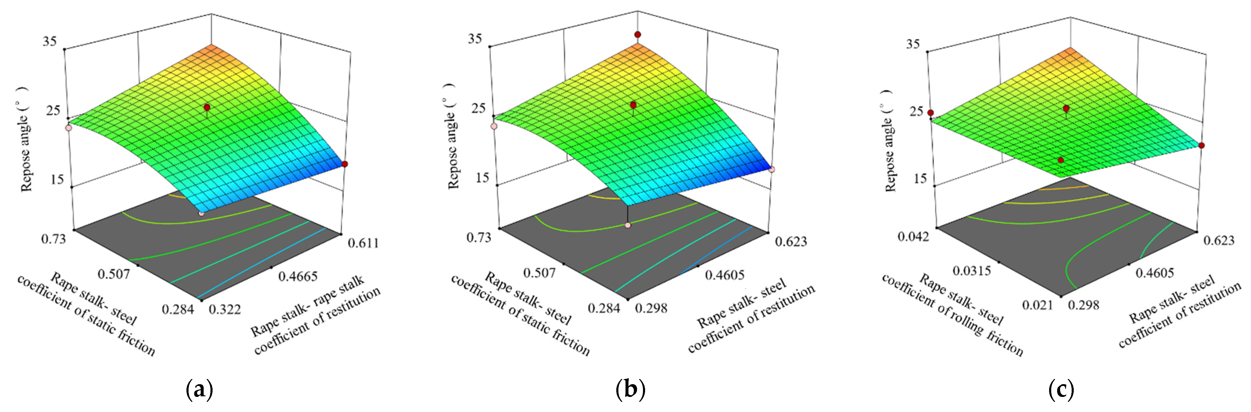
3.1.2. Significant Factor for Repose Angle

The Plackett–Burman simulation test results for the rape stems’ contact parameters are shown in

Table 3. Results of Plackett–Burman simulation test of rape stems’ contact paramaters.

Test No.	A	B	C	D	E	F	y1
1	0.611	0.752	0.032	0.298	0.284	0.021	21.29
2	0.611	0.381	0.013	0.298	0.73	0.021	25.58
3	0.4665	0.5665	0.0225	0.4605	0.507	0.0315	27.18
4	0.611	0.752	0.013	0.298	0.284	0.042	24.89
5	0.611	0.381	0.032	0.623	0.73	0.021	30.33
6	0.611	0.752	0.013	0.623	0.73	0.042	33.60
7	0.4665	0.5665	0.0225	0.4605	0.507	0.0315	26.95
8	0.322	0.381	0.013	0.623	0.284	0.042	24.45
9	0.322	0.752	0.032	0.623	0.284	0.021	20.78
10	0.322	0.752	0.032	0.298	0.73	0.042	25.17
11	0.322	0.381	0.032	0.298	0.73	0.042	34.36
12	0.322	0.752	0.013	0.623	0.73	0.021	26.11
13	0.611	0.381	0.032	0.623	0.284	0.042	25.26
14	0.322	0.381	0.013	0.298	0.284	0.021	17.69

Note: A is rape stem–rape stem coefficient of restitution; B is rape stem–rape stem coefficient of static friction; C is rape stem–rape stem coefficient of rolling friction; D is rape stem–steel coefficient of restitution; E is rape stem–steel coefficient of static friction; F is rape stem–steel coefficient of rolling friction; y₁ is repose angle, (°).

. The test results were subjected to ANOVA to obtain the effect of each parameter, as shown in

Table 4. ANOVA of Plackett–Burman test.

Factor	Standardized Effects	Sum of Squares	Contribution/%	Significance Ranking
A	2.065	12.793	4.305	3
B	−0.972	2.832	0.953	5
C	0.813	1.985	0.668	6
D	1.925	11.117	3.741	4
E	6.800	138.720	46.687	1
F	4.328	56.203	18.916	2

.

According to Table 4, the significance ranking of the repose angles’ effect on the contact parameters of the rape stems was E, F, A, D, B, and C. t-test and Pareto charts (Figure 10) were created to determine the parameters that needed to be further discussed.

As shown in the Pareto charts, the t-value of the coefficient of static friction (E), the rape stem–steel coefficient of the rolling friction contact plasticity ratio (F), the rape stem–rape stem coefficient of restitution (A), and the rape stem–steel coefficient of restitution (D) were all larger than 1, which shows they are the significance fartors for the repose angle. The rape stem–rape stem coefficient of static friction (B) and rape stem–rape stem coefficient of rolling friction (C) had almost no effect on the repose angle. Therefore, E, F, A, and D were the test factors for the further response surface test. For B and C, the intermediate values were taken as 0.5665 and 0.0225, respectively.

3.1.3. Contact Parameter Calibration

The rape stems’ contact parameter response surface simulation test results are shown in

Table 5. Results of rape stems’ contact-parameter-response surface simulation test.

Test No.	A	D	E	F	y1
1	0.322	0.298	0.507	0.0315	22.88
2	0.611	0.298	0.507	0.0315	23.88
3	0.322	0.623	0.507	0.0315	22.77
4	0.611	0.623	0.507	0.0315	25.91
5	0.4665	0.4605	0.284	0.021	17.98
6	0.4665	0.4605	0.73	0.021	24.72
7	0.4665	0.4605	0.284	0.042	23.88
8	0.4665	0.4605	0.73	0.042	31.40
9	0.322	0.4605	0.507	0.021	22.35
10	0.611	0.4605	0.507	0.021	26.12
11	0.322	0.4605	0.507	0.042	27.40
12	0.611	0.4605	0.507	0.042	27.35
13	0.4665	0.298	0.284	0.0315	18.58
14	0.4665	0.623	0.284	0.0315	17.98
15	0.4665	0.298	0.73	0.0315	23.79
16	0.4665	0.623	0.73	0.0315	31.40
17	0.322	0.4605	0.284	0.0315	20.41
18	0.611	0.4605	0.284	0.0315	19.08
19	0.322	0.4605	0.73	0.0315	23.87
20	0.611	0.4605	0.73	0.0315	29.72
21	0.4665	0.298	0.507	0.021	27.25
22	0.4665	0.623	0.507	0.021	21.82
23	0.4665	0.298	0.507	0.042	26.19
24	0.4665	0.623	0.507	0.042	29.29
25	0.4665	0.4605	0.507	0.0315	27.18
26	0.4665	0.4605	0.507	0.0315	24.72
27	0.4665	0.4605	0.507	0.0315	27.01

. The ANOVA of the test results is shown in

Table 6. ANOVA for contact-parameter-response surface test’s results.

Source	Coefficient Estimate (Coded Factors)	Sum of Squares	df	Mean Square	F-Value	p-Value
Model	\	349.62	14	24.97	11.66	<0.0001 **
A	1.03	12.8	1	12.8	5.97	0.0309 *
D	0.5515	3.65	1	3.65	1.70	0.2163
E	3.92	183.94	1	183.94	85.85	<0.0001 **
F	2.11	53.2	1	53.20	24.83	0.0003 **
AD	0.5345	1.14	1	1.14	0.53	0.4792
AE	1.80	12.89	1	12.89	6.02	0.0304 *
AF	−0.9551	3.65	1	3.65	1.70	0.2164
DE	2.05	16.84	1	16.84	7.86	0.0159 *
DF	2.13	18.19	1	18.19	8.49	0.013 *
EF	0.1959	0.1535	1	0.154	0.072	0.7935
A²	−1.10	6.47	1	6.47	3.02	0.1077
D²	−1.10	6.47	1	6.47	3.02	0.1078
E²	−2.22	26.23	1	26.23	12.24	0.0044 **
F²	0.6495	2.25	1	2.25	1.05	0.3257
Intercept	26.30	\	\	\	\	\
Residual	\	25.71	12	2.14	\	\
Lack of Fit	\	21.94	10	2.19	1.16	0.5479
Pure Error	\	3.77	2	1.89	\	\
Cor Total	\	375.33	26		\	\

Note: ** means highly significant (p < 0.01), * means significant (0.01 ≤ p < 0.05).

.

According to the quadratic multi-variate fitting regression ANOVA results of the coefficient of variation y₁, the regression model’s p-values are less than 0.01, which indicates that the model is highly significant. The lack-of-fit F-value is more than 0.05, which implies the model is not significant relative to the pure error. It indicates that the model can correctly reflect the relationship among y₁ and A, D, E, and F as well as predict test results. Among them, A, E, F, and E², are highly significant model terms and AE, DE, and DF are significant model terms. After excluding the insignificant factors, the quadratic regression model (actual factor) of the repose angle y₁ is:

y₁ = 40.03 − 21.00 A + 4.38 E − 375.02 F + 55.71 AE + 56.62 DE + 1249.82 DF − 38.34 E²

(11)

The effect of the interaction factors on the repose angle is shown in Figure 11. When D and F are at the center level (0.4605 and 0.0315), y₁ increases with the increase of A and E. The response surface’s curve changes faster along the E direction, and the effect of the rape stem–steel coefficient of static friction on the repose angle is more significant than that of the rape stem–rape stem coefficient of restitution. When A and F are at the center level (0.4665 and 0.507), y₁ increases with the increase of D and E. The response surface’s curve changes faster along the F direction, and the effect of the rape stem–steel coefficient of static friction on the repose angle is more significant than that of the rape stem-steel coefficient of restitution. When A and E are at the center level (0.4665 and 0.0315), y₁ increases with the increase of D and F. The response surface curve changes faster along the F direction, and the effect of the rape stem–steel coefficient of rolling friction on the repose angle is more significant than that of the rape stem–steel coefficient of restitution.

Using the physical test measurement of the stacking angle of 27.15° as the optimization target, the combination of the contact parameters’ optimization model is:

$$\left\{\begin{array}{l}{y}_1=27.15°\\ \mathrm{s}.\mathrm{t}.\left\{\begin{array}{l}0.322\le A\le 0.611\\ 0.298\le D\le 0.623\\ 0.284\le E\le 0.730\\ 0.021\le F\le 0.042\end{array}\right.\end{array}\right.$$

(12)

Based on Equations (11) and (12), the solution for the optimal combination of parameters was solved as A = 0.514, D = 0.463, E = 0.568, and F = 0.029. The rape stem repose angle simulation result was 26.55° through this combination of parameters. The relative error to the measured values from physical tests (27.15°) was 2.2%.

3.2. Flexible DEM Model

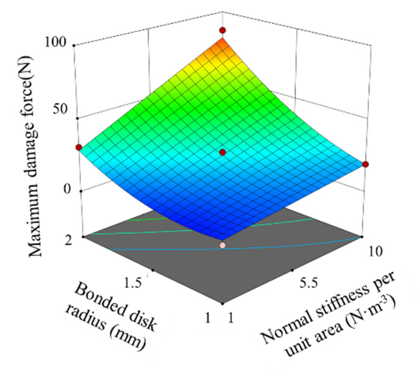
3.2.1. Bonding Parameter Box–Behnken Simulation Test

The result of the bonding parameters’ Box–Behnken simulation is shown in

Table 7. Bonding parameter Box–Behnken simulation result.

Test No.	G/N·m−3	H/N·m−3	I/mm	y2/N
1	5.50 × 109	1.00 × 109	2.0	54.80
2	5.50 × 109	1.00 × 109	1.0	16.16
3	1.00 × 1010	1.00 × 108	1.5	35.90
4	1.00 × 109	1.00 × 108	1.5	8.72
5	5.50 × 109	5.50 × 108	1.5	27.60
6	1.00 × 109	5.50 × 108	1.0	4.91
7	5.50 × 109	5.50 × 108	1.5	27.90
8	1.00 × 1010	5.50 × 108	2.0	86.50
9	5.50 × 109	1.00 × 108	2.0	47.80
10	1.00 × 1010	5.50 × 108	1.0	19.26
11	5.50 × 109	5.50 × 108	1.5	25.30
12	1.00 × 1010	1.00 × 109	1.5	41.80
13	5.50 × 109	1.00 × 108	1.0	14.51
14	1.00 × 109	5.50 × 108	2.0	31.20
15	1.00 × 109	1.00 × 109	1.5	12.43

Note: G is normal stiffness per unit area, N·m⁻³; H is shear stiffness per unit area, N·m⁻³; I is bonded disk radius, mm; y₂ is maximum damage force, N.

. A quadratic multivariate fitting of the experimental results was carried out by applying Design-Expert 12 software, and an ANOVA and a regression coefficient significance test were carried out for the regression model. The result is shown in

Table 8. ANOVA for bonding parameter Box–Behnken simulation result.

Source	Coefficient Estimate (Coded Factors)	Sum of Squares	df	Mean Square	F-Value	p-Value
Model	\	6184.30	9	687.14	40.93	0.0004 **
G	15.77	1990.80	1	1990.80	118.59	0.0001 **
H	2.28	41.68	1	41.68	2.48	0.1759
I	20.68	3422.13	1	3422.13	203.86	<0.0001 **
GH	0.5475	1.20	1	1.20	0.0714	0.7999
GI	10.24	419.23	1	419.23	24.97	0.0041 **
HI	1.34	7.16	1	7.16	0.4263	0.5426
G²	−0.0354	0.0046	1	0.0046	0.0003	0.9874
H²	−2.19	17.63	1	17.63	1.05	0.3524
I²	8.57	271.15	1	271.15	16.15	0.0101 *
Intercept	26.93	\	\	\	\	\
Residual	\	83.93	5	16.79
Lack of Fit	\	79.89	3	26.63	13.16	0.0714
Pure Error	\	4.05	2	2.02	\	\
Cor Total	\	6268.24	14	\	\	\

Note: ** means highly significant (p < 0.01), * means significant (0.01 ≤ p < 0.05).

.

According to Table 8, the regression model’s p-value is less than 0.01, which indicates that the model is very significant. The lack of fit F-value is more than 0.5, which implies that the model is not significant relative to the pure error. It indicates that the model can correctly reflect the relationship among y₂ and G, H, and I as well as predict the test results. Among them, G, I, and GI are highly significant model terms and I² is a significant model term. After excluding the insignificant factors, the quadratic regression model (actual factor) of the maximum damage force y₂ is:

y₂ = 57.64 − 3.32 × 10⁻⁹G − 88.40I + 4.55 × 10⁻⁹GI + 34.91I²

(13)

The effect of the interaction factors on the maximum damage force is shown in Figure 12. When H is at the center level (5.50 × 10⁸), y₂ increases with the increase of G and I. The response surface curve changes faster along the I direction, and the effect of the bonded disk radius on the maximum damage force is more significant than that of normal stiffness per unit area.

Using the physical test measurement of the maximum damage force, 16.20 N, as the optimization target, the combination of the bonding parameters’ optimization model is:

$$\left\{\begin{array}{l}{y}_1=16.2\mathrm{N}\\ \mathrm{s}.\mathrm{t}.\left\{\begin{array}{l}1.0\times {10}^9\le G\le 1.0\times {10}^{10}\\ 1.0\times {10}^8\le H\le 1.0\times {10}^9\\ 1.0\mathrm{m}\mathrm{m}\le I\le 2.0\mathrm{m}\mathrm{m}\end{array}\right.\end{array}\right.$$

(14)

Based on Equations (13) and (14), the solution for the optimal combination of parameters was solved as G = 4.4 × 10⁹ N m⁻³, H = 7.73 × 10⁸ N m⁻³, and I = 1.26 mm.

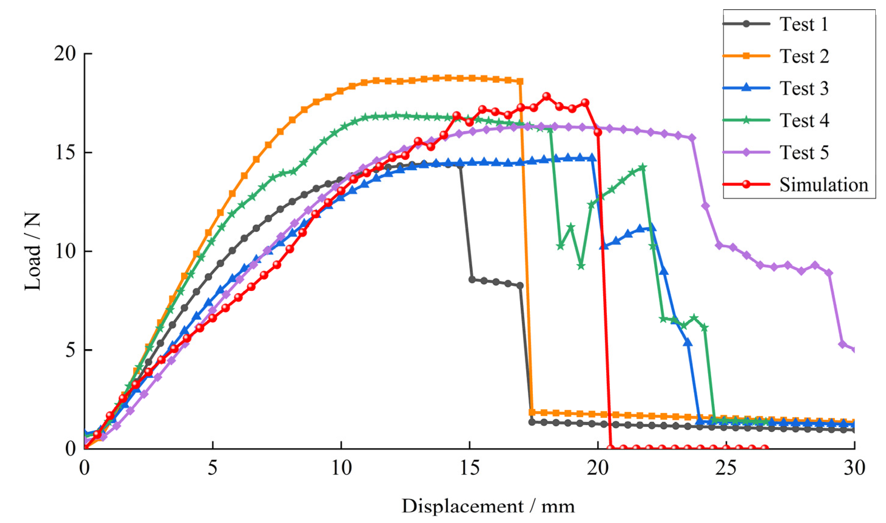
3.2.2. Test Verification

The developed rape-stem flexibility discrete element model and its parameter combinations were used for the three-point bending verification test. The comparison of the displacement-force curve of the simulation with the physical test is shown in Figure 13. The load–displacement curve obtained from the simulation is consistent with the trend of the physical test curves. The load states of the rape stems at each stage were also consistent between the simulation and physical tests. The simulation result of the rape stems’ maximum damage force was 16.76 N, and the relative error of the measured values from the physical tests was 3.5%. The verification test shows that the calibrated flexible discrete element model’s bonding parameters are accurate for rape stems and can be used for simulations of deformation and fracturing under the action of an external force.

3.2.3. Process of Rape Stem Bending and Rupture

According to Figure 13, the rape stem-bending process can be divided into three stages, namely, compression, bending, and rupture. In the stage of compression, the central axis of the stem remains stable under the support of the mechanical tissue of the rape stem, and only a small local compression deformation occurs between the tool and the supporter. There were some differences in the elastic moduli of the rape stem samples, so the actual bending tests had different compression deformation rates, but the bending load always increased rapidly with the increase in the tool displacement. The compression deformation rate of the simulation is relatively small but still within the realistic range. In the stage of bending, the stem is further deformed by compression and the central axis of the stem is bent, resulting in plastic deformation. The loads extracted from both the physical tests and simulations showed a fluctuating lifting trend under the axial tension of the stem. In the stage of rupture, the load exceeds the bending strength of the rape stem and fractures occur in the radial direction of the stem away from the tool. The stem’s cross-sectional morphology is destroyed, and the load after the stem’s rupture falls rapidly until the stem is completely ruptured.

4. Conclusions

In this research, a flexible DEM model for rape stems was developed. The proposed model consists of sequentially arranged rigid units that were bonded together by the Hertz–Mindlin with Bonding contact model in the EDEM. The flexible DEM model could demonstrate the deformation and fracture of the rape stems under external force.

The contact parameter ranges of the rape stems were determined by a bench test and calibrated based on the repose angle. The significant factors for the repose angle were static friction, the rape stem–steel coefficient of rolling friction’s contact plasticity ratio, the rape stem–rape stem coefficient of restitution, and the rape stem–steel coefficient of restitution, and the optimal combination of the parameters was 0.568, 0.029, 0.514, and 0.463, respectively. The repose angle’s simulation result relative error to the physical tests was 2.2%.

The rape stems’ flexible DEM model’s bonding parameters were calibrated based on the three-point bending physical test and the Box–Behnken simulation test. The optimal combination of bonding parameters was obtained as G = 4.40 × 10⁹ N/m³, H = 7.73 × 10⁸ N m⁻³, and I = 1.26 mm. The test results show that the rape stems’ maximum damage force obtained from the constructed model was 16.76 N, and the relative error of the measured values from the physical tests was 3.5%.

The load–displacement curve obtained from the simulation is consistent with the trend of the physical test curves. The load states of the rape stems at each stage were also consistent between the simulation and physical tests. The developed rape-stem flexible DEM model can be used for the simulation of harvesting processes such as cutting, conveying, and threshing.

References

1. Liu, C.; Feng, Z.C.; Xiao, T.H.; Ma, X.M.; Zhou, G.S.; Huang, F.H.; Li, J.N.; Wang, H.Z. Development, potential and adaptation of Chinese rapeseed industry. Chin. J. Oil Crop Sci. 2019, 41, 485–489. [Google Scholar]
2. Guan, Z.H.; Wu, C.Y.; Li, Y.; Mu, S.L.; Jiang, L. Cutting speed follow-up adjusting system of bidirectional electric drive side cutter for rape combine harvester. Sci. Prog. 2020, 103, 0036850420935728. [Google Scholar] [CrossRef] [PubMed]
3. Ma, Z.; Li, Y.M.; Xu, L.Z. Theoretical analysis of micro-vibration between a high moisture content rape stalk and a non-smooth surface of a reciprocating metal cleaning screen matrix. Biosyst. Eng. 2015, 129, 258–267. [Google Scholar] [CrossRef]
4. Guan, Z.H.; Jiang, T.; Li, H.T.; Wu, C.Y.; Zhang, M.; Wang, G.; Mu, S.L. Analysis and test of the laying quality of inclined transportation rape windrower. Trans. Chin. Soc. Agric. Eng. 2021, 37, 59–68. [Google Scholar]
5. Tang, Z.; Li, Y.; Li, X.Y.; Xu, T.B. Structural damage modes for rice stalks undergoing threshing. Biosyst. Eng. 2019, 186, 323–336. [Google Scholar] [CrossRef]
6. Dai, F.; Song, X.; Zhao, W.; Han, Z.; Zhang, F.; Zhang, S. Motion simulation and test on threshed grains in tapered threshing and transmission device for plot wheat breeding based on CFD-DEM. Int. J. Agric. Biol. Eng. 2019, 12, 66–73. [Google Scholar] [CrossRef] [Green Version]
7. Ma, Z.; Li, Y.M.; Xu, L.Z.; Chen, J.; Zhao, Z.; Tang, Z. Dispersion and migration of agricultural particles in a variable-amplitude screen box based on the discrete element method. Comput. Electron. Agric. 2017, 142, 173–180. [Google Scholar] [CrossRef]
8. Yuan, J.C.; Wang, C.; He, K.; Wan, X.Y.; Liao, Q.X. Effect of components mass ratio under sieve on cleaning system performance for rape combine harvester. J. Jilin Univ. Eng. Technol. Ed. 2021, 51, 1897–1907. [Google Scholar]
9. Xu, L.Z.; Wei, C.C.; Liang, Z.W.; Chai, X.Y.; Li, Y.; Liu, Q. Development of rapeseed cleaning loss monitoring system and experiments in a combine harvester. Biosyst. Eng. 2019, 178, 118–130. [Google Scholar] [CrossRef]
10. Lei, X.L.; Liao, Y.T.; Liao, Q.X. Simulation of seed motion in seed feeding device with DEM-CFD coupling approach for rapeseed and wheat. Comput. Electron. Agric. 2016, 131, 29–39. [Google Scholar] [CrossRef]
11. Wan, X.Y.; Liao, Q.X.; Xu, Y.; Yuan, J.C.; Li, H.T. Design and evaluation of cyclone separation cleaning devices using a conical sieve for rape combine harvesters. Appl. Eng. Agric. 2018, 34, 677–686. [Google Scholar] [CrossRef]
12. Schramm, M.; Tekeste, M.Z. Wheat straw direct shear simulation using discrete element method of fibrous bonded model. Biosyst. Eng. 2022, 213, 1–12. [Google Scholar] [CrossRef]
13. Liu, F.Y.; Zhang, J.; Chen, J. Modeling of flexible wheat straw by discrete element method and its parameter calibration. Int. J. Agric. Biol. Eng. 2018, 11, 42–46. [Google Scholar] [CrossRef] [Green Version]
14. Leblicq, T.; Smeets, B.; Vanmaercke, S.; Ramon, H.; Saeys, W. A discrete element approach for modelling bendable crop stems. Comput. Electron. Agric. 2016, 124, 141–149. [Google Scholar] [CrossRef]
15. Liao, Y.T.; Liao, Q.X.; Zhou, Y.; Wang, Z.T.; Jiang, Y.J.; Liang, F. Parameters Calibration of Discrete Element Model of Fodder Rape Crop Harvest in Bolting Stage. Trans. Chin. Soc. Agric. Mach. 2020, 51, 73–82. [Google Scholar]
16. Liu, Z.P.; Xie, F.P.; Wu, M.L. Experimental Study on Mechanics Characteristic for Mature Rape Stalk. J. Agric. Res. 2009, 31, 147–149. [Google Scholar]
17. Luo, H.F.; Tang, C.Z.; Guan, C.Y.; Wu, M.L.; Xie, F.P.; Zhou, Y. Plant characteristic research on field rape based on mechanized harvesting adaptability. Trans. Chin. Soc. Agric. Eng. 2010, 26, 61–66. [Google Scholar]
18. Ma, Z.; Li, Y.M.; Xu, L.Z. Experimental research of Elastic Mechanics of rape stalks. J. Agric. Res. 2016, 38, 187–191. [Google Scholar]
19. Sun, J.B.; Liu, Q.; Yang, F.Z.; Liu, Z.J.; Wang, Z. Calibration of Discrete Element Simulation Parameters of Sloping Soil on Loess Plateau and Its Interaction with Rotary Tillage Components. Trans. Chin. Soc. Agric. Mach. 2022, 53, 63–73. [Google Scholar]
20. Xing, J.J.; Zhang, R.; Wu, P.; Zhang, X.R.; Dong, X.H.; Chen, Y.; Ru, S.F. Parameter calibration of discrete element simulation model for latosol particles in hot areas of Hainan Province. Trans. Chin. Soc. Agric. Eng. 2020, 36, 158–166. [Google Scholar]
21. Chen, Z.P.; Wassgren, C.; Veikle, E.; Ambrose, K. Determination of material and interaction properties of maize and wheat kernels for DEM simulation. Biosyst. Eng. 2020, 147, 206–225. [Google Scholar] [CrossRef]
22. Liu, F.Y.; Zhang, J.; Li, B.; Chen, J. Calibration of parameters of wheat required in discrete element method simulation based on repose angle of particle heap. Trans. Chin. Soc. Agric. Eng. 2016, 32, 247–253. [Google Scholar]
23. Xia, Y.D.; Klinger, J.; Bhattacharjee, T.; Thompson, V. The elastoplastic flexural behaviour of corn stalks. Biosyst. Eng. 2022, 216, 218–228. [Google Scholar] [CrossRef]
24. Wu, K.; Song, Y.P. Research Progress Analysis of Crop Stalk Cutting Theory and Method. Trans. Chin. Soc. Agric. Eng. 2022, 53, 1–20. [Google Scholar]
25. Guo, L.; Wang, D.C.; Tabil, L.G.; Wang, G.H. Compression and relaxation properties of selected biomass for briquetting. Biosyst. Eng. 2016, 148, 101–110. [Google Scholar] [CrossRef]
Figure 1. Rape stem contact parameters test bench. (1) Material box, (2) Baffle plate, (3) Test plate angle adjustment device, (4) Test plate, (5) Frame, (6) Base plate angle adjustment device, and (7) base plate.
Applsci 12 08394 g001
Figure 2. Test of the rape stems’ coefficient of restitution. h1 is the vertical distance between the baffle plate and the center of the test plate, m; α is the angle between the test plate and the horizon, (°); h2 is the vertical distance between the test plate and the base plate m; v1 is the normal fractional velocity of rape stem before the collision, m/s; v2 is the normal fractional velocity of rape stem after the collision, m/s; S is the horizontal distance between rape stem–bottom plate contact point and the center of the test plate, m.
Applsci 12 08394 g002
Figure 3. Coefficient of static friction test method. θs is the friction angle, (°).
Applsci 12 08394 g003
Figure 4. Coefficient of rolling friction test method. θr is the angle between base plate and frame, (°); Gs is rape stem gravity, N; Ff is rolling resistance, N; M1 is rolling torque, N·m; M2 is rolling resistance torque, N·m.
Applsci 12 08394 g004
Figure 5. Rape stem repose angle test. (a) Physical test; (b) Simulation test.
Applsci 12 08394 g005
Figure 6. Rape stem repose angle test. (a) Diameter = 6.0 mm; (b) Diameter = 7.0 mm; (c) Diameter = 4.0 mm.
Applsci 12 08394 g006
Figure 7. Rape stem flexible discrete element model. (a) Rigid discrete unit; (b) Rigid discrete element model; (c) Flexible discrete element model.
Applsci 12 08394 g007
Figure 8. Rape stem three-point bending test: (a) Physics test; (b) Simulation test.
Applsci 12 08394 g008
Figure 9. Rape stem repose angle test. (a) Image of rape stem pile; (b) Binarized image; (c) Boundary Fitting; (d) Test result.
Applsci 12 08394 g009aApplsci 12 08394 g009b
Figure 10. Pareto charts.
Applsci 12 08394 g010
Figure 11. The effect of interaction factors on repose angle: (a) y1 = f (A 0.4605, E, 0.0315); (b) y1 = f (0.4665, D, E, 0.507); (c) y1 = f (0.4665, D, 0.0315, F).
Applsci 12 08394 g011
Figure 12. The effect of interaction factors on maximum damage force. y2 = f (G, 5.50 × 10⁸, I).
Applsci 12 08394 g012
Figure 13. Displacement–force variation curve of rape stems under three-point bending.
Applsci 12 08394 g013