Generation of Controlled Synthetic Samples and Impact of Hyper-Tuning Parameters to Effectively Classify the Complex Structure of Overlapping Region

Abstract

The classification of imbalanced and overlapping data has provided customary insight over the last decade, as most real-world applications comprise multiple classes with an imbalanced distribution of samples. Samples from different classes overlap near class boundaries, creating a complex structure for the underlying classifier. Due to the imbalanced distribution of samples, the underlying classifier favors samples from the majority class and ignores samples representing the least minority class. The imbalanced nature of the data—resulting in overlapping regions—greatly affects the learning of various machine learning classifiers, as most machine learning classifiers are designed to handle balanced datasets and perform poorly when applied to imbalanced data. To improve learning on multi-class problems, more expertise is required in both traditional classifiers and problem domain datasets. Some experimentation and knowledge of hyper-tuning the parameters and parameters of the classifier under consideration are required. Several techniques for learning from multi-class problems have been reported in the literature, such as sampling techniques, algorithm adaptation methods, transformation methods, hybrid methods, and ensemble techniques. In the current research work, we first analyzed the learning behavior of state-of-the-art ensemble and non-ensemble classifiers on imbalanced and overlapping multi-class data. After analysis, we used grid search techniques to optimize key parameters (by hyper-tuning) of ensemble and non-ensemble classifiers to determine the optimal set of parameters to enhance the learning from a multi-class imbalanced classification problem, performed on 15 public datasets. After hyper-tuning, 20% of the dataset samples are synthetically generated to add to the majority class of each respective dataset to make it more overlapped (complex structure). After the synthetic sample’s addition, the hyper-tuned ensemble and non-ensemble classifiers are tested over that complex structure. This paper also includes a brief description of tuned parameters and their effects on imbalanced data, followed by a detailed comparison of ensemble and non-ensemble classifiers with the default and tuned parameters for both original and synthetically overlapped datasets. We believe that the underlying paper is the first kind of effort in this domain, which will furnish various research aspects to with a greater focus on the parameters of the classifier in the field of learning from imbalanced data problems using machine-learning algorithms.

1. Introduction

Learning from imbalanced data [1] has proven its significance through the efforts devoted by the research community over the last couple of years. Most real-world applications such as medical diagnosis, protein classification, activity recognition, target detection, target detection, microarray research, video streaming, and mining are imbalanced [1]. In an imbalanced distribution, the samples of one class outperform the other class or classes of samples with numbers, obviously a hurdle for the traditional classifiers to learn from multi-class problems. Most traditional classifiers [2], such as k-nearest neighbor (kNN), naive Bayes (NB), artificial neural network (ANN), decision tree (TD), support vector machine (SVM), and logistic regression (LR) designed for the balanced and linear distribution of the instances in the training dataset between the classes. In the scenarios, multi-class imbalance learning requires more expertise and skills, since as with the number of classes in the problem domain increases, so do the challenges of representing the whole problem space accurately. Several problems reported in learning from multi-class imbalance data are the majority and minority class and classes problems [1], issues of overlapping class boundaries [3], a small sample size in the minority class [4], and small disjuncts issues [5], which must be taken into account before applying any multi-class imbalance classifier. Different papers discussed these four-fold reasons as a challenge when conventional classifiers are subject to learning from the imbalanced nature of data.

• Traditional classifiers are well designed and indeed have better performance and accuracy over the balanced training set, resulting in sub-optimal classification performance when applied to imbalanced problems [6].
• With the skewed distribution, the predicted accuracy persuades a bias to the class having a greater number of samples, by ignoring the rare class instances, even with the best overall precision produced by the prediction model [7].
• Both the noise and minority class samples are least represented, and the learning models are sometimes confused with each other, whilst noise may be incorrectly recognized as minority instances [8].
• Learning from imbalanced distribution is somehow comfortable if the classes are linearly separable from each other. However, in multi-class imbalanced problems, minority instances are overlapped with each other’s boundaries where the earlier likelihood of both the majority and minority classes are nearly equal [9].

Several approaches were reported in the literature to cope with this imbalanced data problem based on the data level methods [10], algorithm adaptation methods [11], and ensemble-based methods [12]. However, the majority of these approaches focused on handling the binary class imbalance problem apparently cannot be directly applied to multi-class imbalance problems, since the decision boundary involves distinguishing between more classes. At the data-level method, the original data are amended to relive the overlapping impact, either by introducing complementary features or data cleansing methods to separate the overlapping classes or merging overlapping classes to form meta classes [13]. However, using the data-level approaches exclusively to address the imbalance and overlapping issues may result in the model overfitting [14] or may lose some useful information [15]. The fundamental changed algorithm cannot be applied as a general method to effectively tackle the overlapping issues in algorithm-based techniques, which modify the current algorithm to deal with the uneven nature of the information and improve the learning of the underlying classifier [16,17]. The choice of base classifiers, the decision-making process, the number of classifiers used for the construction of an ensemble, the accuracy of individual models, the diversity among the individual models in an ensemble, and the number of classifiers used are some main factors to be carefully studied in an ensemble-based method [18].

Parameter hyper-tuning [19] in the selected model is the process of ascertaining some particular parameters to optimize the performance of learning algorithms on a specific set. Parameter tuning has proven its vital role in improving the accuracy and overall model performance both for ensemble and non-ensemble classifiers [20,21]. Every classifier has its own set of parameters and needs to tune following the different tuning steps by performing an exhaustive grid search. There are two types of model parameters in every machine-learning algorithm, conventional parameters and hyper-parameters. Conventional parameters are optimized during the training phase of the underlying model, whereas the users, depending upon the problem dataset before the training phase of the model, set hyper-parameter values. In the more complex structure, i.e., with the increasing overlapping samples, the needs for the optimal set of parameters become more in order to maximize the visibility of the minority class samples [22].

The key contribution of the underlying paper is to focus on analyzing the learning performance of ensemble and non-ensemble classifiers over multi-class imbalanced and overlapped data. A detailed investigation of ensemble and non-ensemble approaches was presented to provide deep insight into the nature of multi-class learning strategies. An exhaustive experiment on the hyper-tuning of six state-of-the-art ensemble and non-ensemble classifiers, to efficiently address the multi-class imbalance datasets issue and comprehensively compare and improve their performance, was performed using four different evaluation metrics for accuracy, namely the overall accuracy (ACC), geometric mean (G-mean) [23], F-measure [12], and the area under curve (AUC) metrics [24]. As a third contribution, an algorithm was designed to synthetically generate overlapping samples in the existing dataset by 20% of the existing samples to make it more complex and overlap to highlight the impact of parameter tuning. The comparison of ensemble and non-ensemble classifiers was carried out on 15 publicly available multi-class imbalanced and overlapped datasets.

The underlying research article is comprised of the following sections. The literature survey is covered in Section 2. The background of ensemble and non-ensemble-based methods are covered in Section 3 and Section 4. In Section 5, we discussed the hyper-tuning of the parameters of the used classifiers in Section 6, and Section 7 discusses the algorithm to synthetically generate the overlapping samples. Section 8 highlights the experimental setup, dataset, and evaluation methods, Section 9 covers the results and discussion. We compare the ensemble and non-ensemble approaches in Section 10 and the article is concluded in Section 11.

2. Related Works

The authors in [25] argued for the significance of ensemble approaches as compared to the sampling methods and individual classifiers when applied to a multi-class imbalanced dataset. The authors compared the ensemble-based approach with the non-ensemble to prove the robustness of ensemble methods. Yao and Wang in [26] combined AdaBoost.NC and AdaBoost with sampling techniques either augmented with or without the decomposition techniques to address the multi-class imbalance problem and highlight that the ensemble approach is more effective than the oversampling and decomposition techniques. Without class decomposition, AdaBoost.NC shows better performance as compared to AdaBoost, but with the increasing number of classes, their performance also decreased gradually. The authors in [26] showed that the shortcomings of sampling methods cannot be avoided by using standard ensemble approaches if the dataset has multiple classes. Despite the increasing number of samples in the positive class by adding some samples through oversampling, the distribution of classes in the data space is still imbalanced, which is dominated by the majority class. Chawla et al. [27] proposed SMOTEBoost, an ensemble-based sampling technique to enhance the conventional SMOTE [28] by mingling it with AdaBoost.M2. The authors applied SMOTE before the base classifier evaluation, and thus, the new instance’s weight is relative to the numbers of samples in the new dataset. After producing the new instances, the original instance’s weight is standardized to generate the new distribution. In every iteration, the instance weight of the minority class increases. The authors in [29] highlighted the outclass performance of bagging as compared to boosting in a multi-class and noisy environment. Furthermore, bagging techniques have to be quickly developed and become more powerful if properly ensemble. Similarly, OverBagging [30] combines the data preprocessing and bagging techniques to manage the class imbalance issue by increasing the positive class cardinality by the duplication of original examples; at the same time, the instance in the majority of negative class is considered in every bag to increase multiplicity.

In [31], SMOTEBagging was proposed to counter multi-class imbalance learning issues by creating every individual bag to be expressively diverse. In every iteration during bag creation, the SMOTE resampling rate is defined and this ratio specifies the positive class instances randomly resampled from the original dataset, and the remaining positive class instances are generated by SMOTE. Barandela et al. proposed UnderBagging for the first time in [31], wherein the negative class instances are arbitrarily condensed at every bootstrap sample to make it equal to the cardinality of the positive class. The basic, simple version of undersampling when merged with bagging-based techniques proves that it is more significant than the more composite solution, such as BalanceCascade [32] and EasyEnsemble [33]. In [34], the authors highlighted an important problem with the ensemble size and ensemble cardinality (number of component classifiers in the final ensemble), as it affects the predictive performance, time, and memory for the classification algorithm when applied to imbalance data and diversity among the component classifier. The boosting ensemble method presented in [35] is one of the prominent methods explicitly based on the complementarity among the component classifier. Through the boosting process, a strong learner built from the collection of different weak learners (weak in the sense of accuracy while being applied on the classification task). In [35], the authors proposed a new ensemble method, twin bounded weighted relaxed support vector machines (TBWRSVM), which is an extension of the weighted relaxed support vector machine (WRSVM) classifier used for class imbalance problems and outliers. The resulting classifier utilizes twin bounded support vector machines (TBSVM), which provides a quick classification method. The authors in [36] have suggested a novel ensemble approach, “Dynamic Ensemble Selection for Multi-class Imbalanced the dataset (DES-MI)” to handle the multi-class problem’s challenge. To improve learning from multi-class problems, the DES-MI model first creates a balanced training set before choosing an appropriate classifier. To compare the accuracy and computational cost of the well-known boosting-based ensemble classifier Xgboost (ensemble-based method), the authors in [37] looked at its general performance, efficiency, competence, and effectiveness while taking into account its sensitivity to the sample size and feature space. The performance of statistical analysis, according to the authors, is greatly improved when parameterizing Xgboost using a Bayesian approach as opposed to utilizing “random forests” and “support vector machines” that are operated on larger sample size.

The authors in [38] described the suitability of data preprocessing techniques to address the data imbalance issues. The authors of this study are of the opinion that a balanced training dataset is more robust for improving the overall performance of the classifier for several base classifiers. Zhang and Mani in [39] proposed a new technique by achieving undersampling through the kNN classifier. Based on the data features of the data distribution, four undersampling methods based on kNN are proposed, namely $Nea{r}_{Miss1}, Nea{r}_{Miss2}, Nea{r}_{Miss3}$ and the “most distant” method, in which a small subset of training data is selected to minimize the skewness in the reaming data. The authors in [40] highlighted that sampling techniques are very clever in dealing with the binary classification problems with two target variables, facing some difficulties when directly applied to solve multi-class classification problems. The authors used the “Mahalanobis Distance-based Over-sampling (MDO)” [41] technique to handle the imbalanced class data with a mixed attribute, introduce generalized singular value decomposition (GSVD) for complex and mixed-type data, augmenting with a resampling scheme applied on the mixed type of attributes to optimize the synthesis of samples. In [42], the authors presented a combination of k-means clustering and “(SMOTE)”, which results in an effective “oversampling method” and effectively overcomes the imbalance ratio between and within classes and avoids noise generation. K-means clustering is a three-step method: clustering, filtering, and sampling to enhance learning from multi-class classification problems. To address the imbalance classification problems, the authors combine “random oversampling” and “random under sampling techniques” in [43] to propose a hybrid sampling SVM approach. By using the undersampling technique, the samples with the least significance were deleted, followed by the oversampling technique to generate some samples in the minority class. In [44], the authors first proposed an optimization classification model (OCM) to deal with the classification problems using evolutionary computation (EC) techniques. In the second step, the authors proposed a novel algorithm, the self-adaptive fireworks algorithm (SaFWA) based on swarm intelligence, to address the optimization problems. To increase the diversity/range of solutions, four candidate solution generation strategies (CSGSs) were merged with SaFWA. In [45], the authors highlighted the multi-class problem solution strategies (decomposition strategies), i.e., transforming imbalance multi-class problems into several classes and designing a separate classifier for each class (binary decomposition is considered to be the most prominent approach for multi-class decomposition). The proposed model has the flexibility to discard the non-competent classifier to improve the robustness of the combination phase. The competency of the classifier is measured by considering the neighborhood of each sample augmenting with selection criteria (with a threshold option) for a classifier corresponding to the minority class in this neighborhood. The authors in [46], proposed the Bayesian learning probabilistic model to improve the performance of Bayesian classification using the combination of a Kalman filter and K-means. The method is applied to a small dataset just for establishing the fact that the proposed algorithm can reduce the time for computing the clusters from the data. The authors in [47] proposed a deep image analysis–based model for glaucoma diagnosis that uses several features to detect the formation of glaucoma in the retinal fundus. The proposed model is combined with SVM, KNN, and NB to investigate the various aspects related to the prediction of glaucoma in retinal fundus images that help the ophthalmologist make better decisions for the human eye. Some of the prominent existing techniques reported in the literature are listed in

Table 1. Weaknesses and Strengths of Existing techniques in the literature.

Solutions	Strength	Weakness
Decomposition strategies [45]	Transform imbalance multi-class problems into several classes and design a separate classifier for each class.	In the case of multiple classes, handling individual classifiers for each class is time consuming.
Optimization classification model (OCM) using evolutionary computation (EC) techniques, Self-adaptive Fireworks Algori3m (SaFWA) based on swarm intelligence [44]	OCM deals with classification problems, and SaFWA deals with optimization problems. To increase the diversity/range of the solutions, four candidate solution generation strategies (CSGSs) merged with SaFWA.	The solution is based on the optimization and diversity solution, but lacks in addressing the increasing impact of overlapping samples.
k-means clustering and (SMOTE) [42]	Results in an effective oversampling method for overcoming the imbalance ratio between and within classes and avoid the noise generation by combining the undersampling and oversampling methods.	Both in the oversampling and undersampling, the samples in the classes were discarded or increased, while our focus was on increasing the samples in the underlying dataset to minimize visibility.
Mahalanobis distance-based oversampling (MDO) with generalized singular value decomposition (GSVD) [41]	To handle the imbalanced class data with a mixed attribute introduces generalized singular value decomposition (GSVD) for complex and mixed-type data, augmenting with a resampling scheme applied on a mixed type of attributes to optimize the synthesis of samples.	Without the decomposition technique, the proposed solution is unable to address overlapping issues.
Data preprocessing techniques with sampling strategies and a KNN classifier augmenting with different $Nea{r}_{Miss}$ and the “most distant” method [38,39]	A balanced training dataset is more robust to improve the overall performance of the classifier for several base classifiers, where a small subset of training data is selected to minimize the skewness in the reaming data.	Focused on preprocessing techniques rather than on hypertonic and synthetic overlapping.
Twin bounded weighted relaxed support vector machines (TBWRSVM) [35]	Handles the imbalance and outlier in the problem domain.	Well designed for classifying imbalanced datasets and identifying outlier samples, but lacking in synthetic overlapping samples.
SMOTEBagging [31]	The proposed method significantly counters the multi-class imbalance learning issues by creating every individual bag to be expressively diverse.	Only targets the minority class samples to bring back equality to the majority class.
BalanceCascade [32]	The negative class instances are arbitrarily condensed at every bootstrap sample to make it equal to the cardinality of the positive class.	Only focuses on sampling techniques to balance the datasets.
Boosting ensemble method [35]	A strong learner is built from the collection of different weak learners (weak in the sense of accuracy while applying the classification task).	Selection of a base learner is a critical job.

.

3. Ensemble-Based Methods

Ensemble learning, also known as multiple classifier systems, has become an influential solution overshadowing not only multi-class imbalance learning but also two-class imbalance problems and standard classification, as discussed in [48] with regard to the boosting algorithms primarily designed for binary classification. In the literature, different researchers agreed on the versatility and effectiveness of ensemble-based learning techniques, where several component classifier predictions were combined to make a final prediction report, improving the performance of individual weak learners with a small training dataset to build an improved classification-learning model. Ensemble approaches were initially introduced in [49,50] in the early 1990s, who presented their view in [51] by arguing that combining multiple classifiers (via an ensemble process) could yield better performance as compared to individual classifiers. Mathematically [52], the performance of each individual classifier over dataset D with M classes is given in Equation (1) as:

$$w_{i,j}=\frac{2p_j^{\left(C_i\right)}}{|D_j|+p_j^{\left(C_i\right)}+q_j^{\left(C_i\right)}}$$

(1)

where $C_i$ represents the performance of an individual classifier with $i=1,2,3,\dots \dots N$ being evaluated on D and a $N\ast M$ matrix W which is defined as:

$$W=\left[\begin{array}{ccc}{\displaystyle W_{1,1}}& {\displaystyle W_{1,2}}& {\displaystyle W_{1,M}}\\ {\displaystyle W_{2,1}}& {\displaystyle W_{2,2}}& {\displaystyle W_{2,M}}\\ {\displaystyle W_{N,1}}& {\displaystyle W_{N,2}}& {\displaystyle W_{N,M}}\end{array}\right]$$

(2)

Each element of $w_{(i,j)}$ is defined in Equation (3), where $D_j$ is the set of instances of the dataset belonging to the class j, and $p_j^{\left(C_i\right)}$ is the number of accurate predications of the classifiers $C_i$ on $D_j$, and $q_j^{\left(C_i\right)}$ are the false or incorrect predications of $C_i$ that an instance belongs to class j. Subsequently, the target class $\widehat{y}$ of each unknown instance x in the test set is computed by Equation (3):

$$\widehat{y}=ar{g}_{j}max\sum _{i=1}^{N}wi,j\chi A(C_i\left(x\right)=j$$

(3)

where function $argmax$ returns the value of the corresponding index to the largest value from the array, $A=[1,2,3,\dots \dots M]$ is the set of unique class labels and $\chi A$ is the characteristic function which takes into account the prediction $j\in A$ of a classifier $C_i$ on an instance x and creates a vector in which the j coordinate takes a value of 1 and the rest takes the value of 0. After several alternatives and improved versions for ensemble classifiers, ensemble methods are nevertheless categorized into three main types, namely boosting, bagging, and stacking. Through the boosting process, a strong learner is built from the collection of different weak learners (weak in the sense of accuracy when applied to the classification task). In boosting-based methods [44], an individual classifier iteratively learns to become specialized on a specific set of the training dataset. The weighted samples from a subset of the training dataset were used to train a component classifier in such a way which emphasizes previously misclassified samples. In boosting methods, experiments piloted on the training set using different learning models to prompt classifiers to produce output. The weight assigning concept is used in the boosting process to assign higher weights or higher costs for each classifier that misclassified the underlying example. Using the approach of the weighted average, the output of each classifier is updated to generate the final output [53]. The basic idea of a boosting-based method is to combine the weak learner to build a strong learner to improve the overall accuracy and performance. Among the boosting family, AdaBoost [54] and Gradient tree boosting [55] are well-known methods of boosting ensemble methods. In a boosting-based method, the resulting ensemble model is defined as the weighted sum of weak learners, as shown in the Equation (4).

$$S_L(.)=\sum _{l=1}^L{C}_l\ast W_l(.)$$

(4)

where $c_{l^{\prime }s}$ are coefficients and $w_{l^{\prime }s}$ are weak learners. Using Equation (4) and finding the best ensemble model is somehow a difficult optimization problem. Instead of using this model approach, we can use an iterative optimization process to find all the coefficients and weak learners that give the best overall additive model by adding the weak learners one by one, looking at each iteration for the best possible pair (coefficient, weak learner) to add to the current ensemble model. We recurrently define the $\left(s_l\right){}^{\prime }s$ as shown in Equation (5):

$$S_l(.)=S_{l-1}(.)+C_l\ast W_l(.)$$

(5)

where $C_l$ and $W_l$ are chosen such that $S_l$ is the model that best fits the training data and therefore is the best possible improvement over $S_{(l-1)}$. We can then denote this in Equation (6):

$$(C_l\ast W_l(.))=ar{g}_{c,w(.)}minE\left(S_{l-1(.)}\right)+(C_l\ast W_l(.))=ar{g}_{c,w(.)}min\sum _{n=1}^{N}e(y_n,S_{l-1}\left(x_n\right))+c\ast w(x)$$

(6)

where $E(.)$ is the fitting error of the given model and $e(., .)$ is the loss/error function. Thus, instead of “globally” optimizing over all the L models in the sum, we approximate the optimum by optimizing “locally” building and adding the weak learners to the strong model one by one.

Bagging methods based on bootstrap aggregation minimize the prediction variance by producing additional examples from the original data for the training set. The training of several base classifiers was carried out on the bootstrap instances of a refined subset of the training dataset, and by using the simple aggregation (majority voting), combines the output of these base classifiers into the final output, thus resulting in a more diverse ensemble, a key factor for an ensemble to work efficiently and effectively. A separate classifier is introduced for each example in the training set, thus having k numbers of a classifier for each iteration of the training set. From the bagging family, the most prominent methods reported in the literature are random forest, which is a flexible and easy-to-use ensemble-based machine-learning algorithm. Most of the time random forest gives very good results, even without hyper-tuned parameters. Because of its simplicity, it can be widely used for both regression and classification tasks. A variation of the bagging scheme, UnderBagging [2], under samples the underlying subset of the instance before the bagging iteration for multi-class imbalance problems by keeping all the minority class samples in each iteration. Another variation of bagging schemes is random forest [5], where the base classifier trained via the bootstrap samples of the underlying training dataset has been randomly reduced to a small subset of dataset samples. In voting-based ensemble methods, predictions from various individual models are combined. In the voting method using an ensemble approach, two or more component models were created separately with a dataset, following an ensemble model to wrap the previously created models and the prediction of those models then aggregated. The resulting model was used to predict new data. Assuming that we have L, bootstrap samples (approximations of L independent datasets) of size B are denoted in Equation (7):

$$\{z_1^1,z_2^1,z_B^1\},\{z_1^2,z_2^2,z_B^2\},\{z_1^L,z_2^L,z_B^L\}$$

(7)

where $z_b^l\equiv b\mathrm{th}$ observation of the $l\mathrm{th}$ bootstrap sample. We can fit L almost independent weak learners (one on each dataset) as given in Equation (8):

$$w_1(.),w_2(.),\dots \dots ,w_L(.)$$

(8)

All the weak learners of Equation (8) are then combined into some kind of averaging process to obtain an ensemble model with a lower variance. For example, we can define our strong model given in Equation (9):

$$S_L(.)=ar{g}_k^{l=1}max\left[card(l\mid w_l(.)=k)\right]$$

(9)

Apart from accuracy improvements and being accuracy oriented, most of the standard techniques for creating ensembles face difficulties in identifying the subset of the dataset with the minority class. To cope with such difficulties, special attention has to pay to designing ensemble algorithms to handle the class imbalance problem. The effective combination of imbalanced learning, ensemble learning techniques with a base learner, and sampling strategies to confront the imbalance class issue put forward many possible proposals for prominent results in the literature by putting aside the conventional categories such as cost-based and kernel-based methods in the imbalanced domain [56]. Regardless of the popularity, versatility, and effectiveness of ensemble methods (by using an independent baseline classifier) as compared to cost-sensitive and improved algorithm-based methods, in an ensemble process, however, transforming dissimilar classifiers by ensuring their stability and regularity using the underlying training dataset is still a crucial factor for ensured accuracy while dealing with the multi-class classification problems. All the symbols used in this article are described in

Table 2. Symbol and their description.

Symbol	Description
$D_j$	Sample of class j
$p_j^{\left(C_i\right)}$	Number of accurate predications of the classifiers i
$\chi A$	Characteristic function which takes into account the prediction $j\in A$
$c_{l^{\prime }s}$	Coefficients
$w_{l^{\prime }s}$	Weak learners
$z_b^l$	b-th observation of the l-th bootstrap sample
L	Bootstrap samples
C	Regularization parameter
$\lambda$	Kernel width parameter
$n_{estimator}$	Number of trees
$lea{f}_{size}$	$lea{f}_{size}$ parameters
K	Neighbor at k distance
$ma{x}_{depth}$	Last leaf node of the tree
$y_i$ and ${\widehat{y}}_i$	Actual value and predicted value of observation i
$C_i$	Class ith sample
$C_j$	Class jth sample
$r_{fi}$	Discriminative ratio
$d(\overrightarrow{\mathrm{a}},\overrightarrow{\mathrm{b}})$	Distance of two vector (two samples of the classes)
$d_i$	Average distance
$k_1$	Nearest neighbors
$N_{ei}$	Sample in the target class
$M{C}_{Count}$	Samples in the majority class
$Col$	Column in the dataset
$Loc$	Location of the sample
S	S Set of synthetic samples
T	T Subset of D (multiclass dataset)
$y_{new}$	New minority
$f_i$	Feature listed in dataset
$Learnin{g}_{rate}$ and $number-of-tree$	The boosting parameters directly related to the underlying boosting algorithm
N	Total number of observations
E(.)	Fitting error
$e(.,.)$	Loss/error function
$S_l$	Model that best fits the training data
$p_{cj}{p}_{ck}$	Represent the respective samples in classes $c_j$ and $c_k$
${\mu }^{f_i}$	Mean of the $f_i$ values across all classes

.

4. Non-Ensemble-Based Methods

Different research papers have empirically and experimentally reported that the classification of a balanced dataset is somewhat elementary and comfortable to perform, but it becomes difficult when the data are not balanced [57]. The standard machine learning algorithm assumes a balanced distribution of classes in a subset of the dataset used for classification; however, the distribution of instances in classes is not uniform in many real-life situations [58]. Traditional classifiers, initially designed for the classification of balanced datasets, show a significant performance for the underlying problem of having a balanced dataset. On the other hand, real-world data are messy with an unequal distribution of samples, where the traditional classifiers fail to properly identify the relevant target class. Figure 1 shows the imbalanced distribution of samples. This imbalance distribution of instances causes biases toward the majority group, thus creating difficulty for the standard learning algorithm to correctly predict an unseen sample. The ignorance of the minority class will lead to building a poor model, as sometimes, this leased-focused class carries important information, thus providing an impractical classifier for our proposed use case. Many standard classification algorithms, namely the SVM, ANN, DT, NB classifier, and KNN, which are designed based on balanced training datasets, become less effective due to skewed distribution in imbalance classes [59]. Although some of them can use for a small dataset as imbalanced data, if we apply the traditional algorithms to multi-class and multi-label problems with an imbalanced dataset, a good performance in terms of accuracy [60] is not necessarily achieved, as standard algorithms are built with the assumption that the distribution is balanced. Therefore, when presented with large imbalanced datasets, these algorithms fail to properly represent the distributive characteristics of data [1]. Classification problems in many real-world applications and scenarios involve multiple classes both in a balanced and in an imbalanced dataset. The learning environment becomes more complex and challenging when the number of classes increases in the domain and multiple classes overlap with each other’s, making it difficult to establish a clear decision boundary between any two classes or among the classes.

4.1. Support Vector Machine Classifier

Using SVM, in the experiment section, we used both the linear and kernel SVM on the stated datasets to classify multi-class imbalanced data. The RBF kernel is used for a decision function in nonlinear SVM [61], as the data are not linearly separable. A set of parameters [62] that need to be hyper-tuned to improve the performance of kernel SVM on multi-class imbalance data are C (a regularisation parameter used to manage or balance the low testing and training error to make a more general algorithm on unseen data), to adjust the decision boundary curvature and hyperplane shape for the class dividing, the gamma $\gamma$ (also known as kernel width parameter), and the decision function (decision function shape) and assigning any weight to a class or classes. Thes small values of C may cause the model to estimate constantly and make it difficult to understand the data; on the other hand, big values of C may cause the model to overfit the training data. Similar to this, the class splitting hyper-shape planes will change for very large values of $\gamma$. If the data in the dataset are not balanced, class-weight balance is employed. The decision function shape decides the decomposition strategy, whether to apply one-versus-one or one-versus-rest. The parameter search range and optimal parameters are shown in

Table 3. Parameters Tuning of the Selected Classifiers for the 9 Datasets.

Algorithm	Tuned Parameter	Search Range	Best P	Dataset
Gradient boosting	Number of estimators	[100; 150; 200; 250; 300; 400; 500; 600; 800; 1000; 1200]	100	IRIS, Car, Counterceptive Used Method, Page_Block, User_Knowledge, Vehicle, Wine, Volcanoes, Wall_Following, Nursey
	Learning rate	[0.01; 0.02; 0.5; 0.1; 0.2; 0.25; 0.3; 0.4; 0.5]	0.5
	Min_samples_split	[2; 3; 4; 5; 6; 8; 10; 15]	2
	Max_tree_depth	[3; 4; 5; 6; 7; 8; 9; 10; 12; 15]	4
Random forest	Number_of_estimators	[50, 120; 150; 200; 220; 250; 300; 350; 600; 700]	200
	Max_features	[‘log2’; ‘sqrt’; ‘all’]	all
	Min_samples_leaf	[1; 2; 3; 4; 5; 6; 7; 8; 9; 10]	2
Decision Tree	‘max_features’:	[‘auto’, ‘sqrt’, ‘log2’, Non]	None
	Criterion	‘gini’, ‘entropy’	gini
	max_depth	1, 20, 2
	Splitter	best’, ’random	best
	‘min_samples_split’:	[2, 5, 10],	5
	‘min_samples_leaf’:	[1, 2, 4, 10],	1
KNN	n_neighbors’:	np.arange (1, 15),	5
	weights’:	[‘uniform’, ‘distance’],	Uniform
	leaf_size’	[1, 3, 5]	3
RBF support vector machine	Gamma	2 × 10−15, 2 × 10−13, 2 × 10−11, 2 × 10−9, 2 × 10−7, 2 × 10−5, 2 × 10−3, 2 × 10−1, 2 × 101, 2 × 1031, 0.1, 0.01, 0.001, 1, 10, 50, 100, 200, 500	100
	C	2 × 10−1, 2 × 101, 2 × 103, 2 × 105, 0.1, 0.01, 1, 10, 100	0.1
	Decision_function_shape	[O-vs-O, O-vs-R]	O-vs-R
	Class_weight	Uniform, balanced	uniform
Logistic regression	Penalty	[2, 6, 8, 12, 15, 16]	12
	Solver	[‘newton-cg’, ‘lbfgs’, ‘liblinear’, ‘sag’, ‘saga’]	‘newton-cg’	For large datasets, ‘sag’ and ‘saga’ will be used

and

Table 4. Parameters Tuning of the Selected Classifiers for the 11 Datasets.

Algorithm	Tuned Parameter	Search Range	Best P	Dataset
Gradient boosting	Number of estimators	[100; 150; 200; 250; 300; 400; 500; 600; 800; 1000; 1200]	200	Soybean, Satimage, Opt_Digits, Glass, LED_Domain, Ecoli, Dermatology, Bridges, Breast_Tissue, Human_Activity_Recognition
	Learning rate	[0.01; 0.02; 0.5; 0.1; 0.2; 0.25; 0.3; 0.4; 0.5]	0.1
	Min_samples_split	[2; 3; 4; 5; 6; 8; 10; 15]	3
	Max_tree_depth	[3; 4; 5; 6; 7; 8; 9; 10; 12; 15]	8
Random forest	Number of estimators	[50, 120; 150; 200; 220; 250; 300; 350; 600; 700]	200
	Max_number of features	[‘log2’; ‘sqrt’; ‘all’]	all
	Min_samples_leaf	[1; 2; 3; 4; 5; 6; 7; 8; 9; 10]	2
Decision tree	‘max_features’:	[‘auto’, ‘sqrt’, ‘log2’, None ]	None
	criterion	’gini’, ’entropy’	gini
	max_depth	1, 20, 2
	splitter	’best’, ’random’	best
	‘min_samples_split’:	[2, 5, 10],	5
	‘min_samples_leaf’:	[1, 2, 4, 10],	1
K-NN	n_neighbors’:	np.arrange (1, 15),	5
	weights’:	[‘uniform’, ‘distance’],	Uniform
	leaf_size’	[1, 3, 5]	5
RBF support vector machine	gamma	2 × 10−15, 2 × 10−13, 2 × 10−11, 2 × 10−9, 2 × 10−7, 2 × 10−5, 2 × 103, 2 × 10−1, 2 × 101, 2 × 1031, 0.1, 0.01, 0.001, 1, 10, 50, 100, 200, 500	200
	C	2 × 10−1, 2 × 101, 2 × 103, 2 × 105, 0.1, 0.01, 1, 10, 100	0.01
	Decision_function_shape	[O-vs-O, O-vs-R]	O-vs-R
	Class_weight	Uniform, balanced	uniform
Logistic regression	penalty	[2, 6, 8, 12, 15, 16]	12
	solver	[‘newton-cg’, ‘lbfgs’, ‘liblinear’, ‘sag’, ‘saga’]	‘newton-cg’	‘saga’ and ‘sag’ will be used for a larger dataset

.

4.2. Random Forest Classifier

To improve the overall model performance via the RF classification model, a set of four parameters needs to be hyper-tuned [63]: the number of $n_{estimator}$ (number of trees), maximum depth, maximum features, and minimum sample split. With regard to the number of tree different opinions there are, some researchers have suggested using the default number of trees to obtain more stable results, whereas some authors argue that a large number of trees should be used. The maximum depth specifies how long the node is expended; if it is not specified, then all nodes will be expended until the leaf node. To achieve the best split, the optimal number of features should be hyper-tuned in the value for ‘max-features’. ‘Minimum-sample-split’ specifies the splitting criteria of an internal node. The parameter search range and optimal parameters are shown in Table 3 and Table 4.

4.3. K-Nearest Neighbor

The basic working procedure of kNN is to find a cluster (subset) of k instances which is the nearest to the predicted sample in the underlying training space, thus showing the independence from the structure of the data. The set of parameters [64] that needs to be tuned to improve the performance of kNN is k, ‘$weights$’, and ‘$lea{f}_{size}$’. The distance between two points is calculated using the Euclidean distance function. The class having majority k-nearest neighbors is the predicted class for the new predicted sample. K is the key parameter to be tuned (after exhaustive grid search) to obtain a satisfactory result. Other important parameters are ‘$weights$’ and ‘$lea{f}_{size}$’, which are weights of two types, namely uniform and distance; for a better prediction accuracy, the uniform weight is considered for the multi-class classification problem, and the ‘$lea{f}_{size}$’ parameter is a key indicator for the speedy construction, query and memory requirement to store the tree.

4.4. Gradient Boosting Algorithm

The parameters of the boosting-based model [65] are sub-categorized into three types, namely parameters specific to a tree structure, boosting specific parameters, and miscellaneous parameters. Since a decision tree is used as a default base learner, parameters specific to the tree structure are allied with each base learner, for example, the sample (minimum number) is requisite to split an interior node or the ‘$ma{x}_{depth}$’ for each tree. ‘$Learnin{g}_{rate}$’ and ‘$\mathit{number-of-tree}$’ are the boosting parameters, directly related to the underlying boosting algorithm.

4.5. Decision Tree Algorithm

Decision trees can apply to both balanced and imbalanced (multi-class) classification and regression problems; however, it best employs a nonlinear decision, with a pre-defined class variable or target label. The decision tree enables a predictive classification model with refined accuracy and precision, and provides better stability to the model with the ease of classification. During our experiment, we hyper-tuned these six parameters [66] to make a significant change to the overall performance of the model, and ‘$criterion$’, ‘$maximu{m}_{depth}$’, ‘$splitter$’, ‘$maximu{m}_{depth}$’, ‘$minimu{m}_{sample-split}$’, ‘$minimu{m}_{sample-leaf}$’ and ‘$maximu{m}_{features}$’. The criterion function will decide the quality of the split; to decide the split at each node, the splitter function is used, and how long the tree should grow will be decided by the maximum depth function, the required sample for an internal node to split will be based on $minimu{m}_{samplesplit}$, the $minimu{m}_{numberofsample}$ required at the leaf node will be decided by the $minimum-sampleleaf$, and $maximu{m}_{featurefunction}$ determines the number of features to be considered when looking for the best split.

4.6. Logistic Regression

Logistic regression can be used for both binary and multi-class imbalance problems [41], although it was initially designed for binary classification, using the one-versus-rest decomposition strategy or modifying the loss function to cross-entropy loss, and logistic regression can be used for multi-class classification. To set the logistic regression for multi-class classification, a parameter called “multi-class” value will be enabled to be multi-class. For multi-class classification, the training model requires the “one-versus-rest” decomposition strategy in case the “multi-class” option is set to “OVR’, and if the “multi-class” option has a “multinomial” value, then “cross-entropy-loss” will be used [67]. The default value of “multi-class” is ‘ovr’, and currently, the ‘multinomial’ can have one of the four possible values as a solver, namely newton-cg, sag, and lbfgs. During the multi-class classification using exhaustive grid search, the two following parameters have proven to be effective for multi-class classification, penalty, and solver with the values, ‘newton-cg’, ‘lbfgs’, ‘liblinear’, ‘sag’, and ‘saga’. ‘liblinear’ is a better option for a dataset that has a lesser number of classes, and if the dataset have a large number of classes ‘saga’ and ‘sag’ are the best choice to use. For multiclass problems, only ‘newton-cg’, ‘sag’, ‘saga’, and ‘lbfgs’ can handle multinomial loss; ‘liblinear’ is limited to one-versus-rest schemes.

5. Parameter Tuning

Parameter tuning is the process of ascertaining some particular parameters to optimize the performance of learning algorithms on a specific set [68] to improve the accuracy and the overall model’s performance both for ensemble and non-ensemble classifiers. Every classifier has its own set of parameters, and needs to tune following the different tuning steps by performing an exhaustive grid search. Most of the time, we assess and compare the underlying models’ performance for the best hyper-parameter settings using the grid search technique and response surface methodology (RSM). However, some researchers [69] have preferred the mean absolute error (MAE) to compare the performance, which is given in Equation (10):

$$MAE=\sum _{i=1}^N\frac{\mid y_i-\widehat{y}\mid }{N}$$

(10)

where $y_i$ and ${\widehat{y}}_i$ and denote the actual value and predicted value of observation i, respectively, $ei$ denotes the prediction error of observation i, and N denotes the total number of observations in the data. The lower the MAE, the better the model performance.

In this article for the individual classifier, we tested a series of values using ten-fold cross-validation [70] and a grid search mechanism for parameter tuning until an optimal parameter set showing the overall highest classification accuracy and precision for each classifier was obtained. In the result section, each classifier was compared with and without tuned parameters on 20 publicly available datasets. The comparison of eight state-of-the-art classifiers (ensemble and non-ensemble) is highlighted in

Table 5. Accuracy and precision before hyper-tuning.

	Accuracy before Hyper-Tuning						Precision before Hyper-Tuning
Datasets	GB	RF	DT	KNN	R-SVM	LR	GB	RF	DT	KNN	R-SVM	LR
IRIS	94.74	97.37	94.74	92.11	92.11	92.11	93.39	96.02	93.39	90.76	90.76	90.76
Glass	94.59	95.32	91.35	94.11	94.11	94.11	93.24	93.97	90	92.76	92.76	92.76
HAR	88.45	87.3	86.2	86.32	86.32	86.32	87.1	85.95	84.85	84.97	84.97	84.97
B_Tissue	95.71	96.57	92.86	88.92	88.92	88.92	94.36	95.22	91.51	87.57	87.57	87.57
Car	86.5	82.89	80.97	81.6	81.6	81.6	85.15	81.54	79.62	80.25	80.25	80.25
CMC	87.21	84.92	81.67	83	83	83	85.86	83.57	80.32	81.65	81.65	81.65
Ecoli	91.98	88.89	88.38	86.86	86.86	86.86	90.63	87.54	87.03	85.51	85.51	85.51
Nursery	82.94	83.67	81.99	88.57	88.57	88.57	81.59	82.32	80.64	87.22	87.22	87.22
Opt_Digits	85.47	86.01	83.19	76.04	76.04	76.04	84.12	84.66	81.84	74.69	74.69	74.69
Page_Block	85.85	83.37	84.41	79.27	79.27	79.27	84.5	82.02	83.06	77.92	77.92	77.92
Satimage	85.53	84.4	85.53	79.66	79.66	79.66	84.18	83.05	84.18	78.31	78.31	78.31
Soyaben	92.35	91.04	89.92	80.65	80.65	80.65	91	89.69	88.57	79.3	79.3	79.3
Vehicle	82.5	83.5	75.36	81.68	81.68	81.68	81.15	82.15	74.01	80.33	80.33	80.33
Volcanoesa	80.81	79	81.9	86.49	86.49	86.49	79.46	77.65	80.55	85.14	85.14	85.14
Wine	96.61	96.61	94.92	78.82	78.82	78.82	95.26	95.26	93.57	77.47	77.47	77.47

,

Table 6. Recall and F1-score before hyper-tuning.

	Accuracy before Hyper-Tuning						Precision before Hyper-Tuning
Datasets	GB	RF	DT	KNN	R-SVM	LR	GB	RF	DT	KNN	R-SVM	LR
IRIS	90.5	93.13	90.5	87.87	87.87	87.87	87.03	89.66	87.03	84.4	84.4	84.4
Glass	90.35	91.08	87.11	89.87	89.87	89.87	86.88	87.61	83.64	86.4	86.4	86.4
HAR	84.21	83.06	81.96	82.08	82.08	82.08	80.74	79.59	78.49	78.61	78.61	78.61
B_Tissue	91.47	92.33	88.62	84.68	84.68	84.68	88	88.86	85.15	81.21	81.21	81.21
Car	82.26	78.65	76.73	77.36	77.36	77.36	78.79	75.18	73.26	73.89	73.89	73.89
CMC	82.97	80.68	77.43	78.76	78.76	78.76	79.5	77.21	73.96	75.29	75.29	75.29
Ecoli	87.74	84.65	84.14	82.62	82.62	82.62	84.27	81.18	80.67	79.15	79.15	79.15
Nursery	78.7	79.43	77.75	84.33	84.33	84.33	75.23	75.96	74.28	80.86	80.86	80.86
Opt_Digits	81.23	81.77	78.95	71.8	71.8	71.8	77.76	78.3	75.48	68.33	68.33	68.33
Page_Block	81.61	79.13	80.17	75.03	75.03	75.03	78.14	75.66	76.7	71.56	71.56	71.56
Satimage	81.29	80.16	81.29	75.42	75.42	75.42	77.82	76.69	77.82	71.95	71.95	71.95
Soyaben	88.11	86.8	85.68	76.41	76.41	76.41	84.64	83.33	82.21	72.94	72.94	72.94
Vehicle	78.26	79.26	71.12	77.44	77.44	77.44	74.79	75.79	67.65	73.97	73.97	73.97
Volcanoesa	76.57	74.76	77.66	82.25	82.25	82.25	73.1	71.29	74.19	78.78	78.78	78.78
Wine	92.37	92.37	90.68	74.58	74.58	74.58	88.9	88.9	87.21	71.11	71.11	71.11

,

Table 7. Accuracy and Precision after Parameters Hyper-Tuning.

	Accuracy before Hyper-Tuning						Precision before Hyper-Tuning
Datasets	GB	RF	DT	KNN	R-SVM	LR	GB	RF	DT	KNN	R-SVM	LR
IRIS	95.71	98.34	95.71	93.08	95.08	87.81	94.36	96.99	94.36	91.73	93.73	86.46
Glass	95.56	96.29	92.32	87.29	89.89	85.34	94.21	94.94	90.97	85.94	88.54	83.99
HAR	89.42	88.27	87.17	82.57	83.97	81.31	88.07	86.92	85.82	81.22	82.62	79.96
B_Tissue	96.68	97.54	93.83	87.83	89.54	81.54	95.33	96.19	92.48	86.48	88.19	80.19
Car	87.47	83.86	81.94	77.01	80.24	71.03	86.12	82.51	80.59	75.66	78.89	69.68
CMC	88.18	85.89	82.64	80.63	81.62	75.87	86.83	84.54	81.29	79.28	80.27	74.52
Ecoli	92.95	89.86	89.35	82.65	87.46	81.04	91.6	88.51	88	81.3	86.11	79.69
Nursery	83.91	84.64	82.96	79.79	81.91	71.68	82.56	83.29	81.61	78.44	80.56	70.33
Opt_Digits	86.44	86.98	84.16	81.57	82.57	76.41	85.09	85.63	82.81	80.22	81.22	75.06
Page_Block	86.82	84.34	85.38	73.82	83.12	74.21	85.47	82.99	84.03	72.47	81.77	72.86
Satimage	86.5	85.37	86.5	76.36	83.79	73.53	85.15	84.02	85.15	75.01	82.44	72.18
Soyaben	93.32	92.01	90.89	86.81	89.48	82.56	91.97	90.66	89.54	85.46	88.13	81.21
Vehicle	83.47	84.47	76.33	67.76	78.13	71.47	82.12	83.12	74.98	66.41	76.78	70.12
Volcanoesa	81.78	79.97	82.87	72.85	75.1	69.94	80.43	78.62	81.52	71.5	73.75	68.59
Wine	97.58	97.58	95.89	83.85	89.2	81.89	96.23	96.23	94.54	82.5	87.85	80.54

,

Table 8. Recall and F1-Score after Parameters Hyper-Tuning.

	Accuracy before Hyper-Tuning						Precision before Hyper-Tuning
Datasets	GB	RF	DT	KNN	R-SVM	LR	GB	RF	DT	KNN	R-SVM	LR
IRIS	90.87	93.5	90.87	88.24	90.24	82.97	87.8	90.43	87.8	85.17	87.17	79.9
Glass	90.72	91.45	87.48	82.45	85.05	80.5	87.65	88.38	84.41	79.38	81.98	77.43
HAR	84.58	83.43	82.33	77.73	79.13	76.47	81.51	80.36	79.26	74.66	76.06	73.4
B_Tissue	91.84	92.7	88.99	82.99	84.7	76.7	88.77	89.63	85.92	79.92	81.63	73.63
Car	82.63	79.02	77.1	72.17	75.4	66.19	79.56	75.95	74.03	69.1	72.33	63.12
CMC	83.34	81.05	77.8	75.79	76.78	71.03	80.27	77.98	74.73	72.72	73.71	67.96
Ecoli	88.11	85.02	84.51	77.81	82.62	76.2	85.04	81.95	81.44	74.74	79.55	73.13
Nursery	79.07	79.8	78.12	74.95	77.07	66.84	76	76.73	75.05	71.88	74	63.77
Opt_Digits	81.6	82.14	79.32	76.73	77.73	71.57	78.53	79.07	76.25	73.66	74.66	68.5
Page_Block	81.98	79.5	80.54	68.98	78.28	69.37	78.91	76.43	77.47	65.91	75.21	66.3
Satimage	81.66	80.53	81.66	71.52	78.95	68.69	78.59	77.46	78.59	68.45	75.88	65.62
Soyaben	88.48	87.17	86.05	81.97	84.64	77.72	85.41	84.1	82.98	78.9	81.57	74.65
Vehicle	78.63	79.63	71.49	62.92	73.29	66.63	75.56	76.56	68.42	59.85	70.22	63.56
Volcanoesa	76.94	75.13	78.03	68.01	70.26	65.1	73.87	72.06	74.96	64.94	67.19	62.03
Wine	92.74	92.74	91.05	79.01	84.36	77.05	89.67	89.67	87.98	75.94	81.29	73.98

,

Table 9. Accuracy and Precision after Parameters Hyper-Tuning and Synthetic Overlapping.

	Accuracy before Hyper-Tuning						Precision before Hyper-Tuning
Datasets	GB	RF	DT	KNN	R-SVM	LR	GB	RF	DT	KNN	R-SVM	LR
IRIS	95.12	97.75	95.12	92.37	94.37	87.1	93.75	96.38	93.75	91.01	93.01	85.74
Glass	94.97	95.7	91.73	86.58	89.18	84.63	93.6	94.33	90.36	85.22	87.82	83.27
HAR	88.83	87.68	86.58	81.86	83.26	80.6	87.46	86.31	85.21	80.5	81.9	79.24
B_Tissue	96.09	96.95	93.24	87.12	88.83	80.83	94.72	95.58	91.87	85.76	87.47	79.47
Car	86.88	83.27	81.35	76.3	79.53	70.32	85.51	81.9	79.98	74.94	78.17	68.96
CMC	87.59	85.3	82.05	79.92	80.91	75.16	86.22	83.93	80.68	78.56	79.55	73.8
Ecoli	92.36	89.27	88.76	81.94	86.75	80.33	90.99	87.9	87.39	80.58	85.39	78.97
Nursery	83.32	84.05	82.37	79.08	81.2	70.97	81.95	82.68	81	77.72	79.84	69.61
Opt_Digits	85.85	86.39	83.57	80.86	81.86	75.7	84.48	85.02	82.2	79.5	80.5	74.34
Page_Block	86.23	83.75	84.79	73.11	82.41	73.5	84.86	82.38	83.42	71.75	81.05	72.14
Satimage	85.91	84.78	85.91	75.65	83.08	72.82	84.54	83.41	84.54	74.29	81.72	71.46
Soyaben	92.73	91.42	90.3	86.1	88.77	81.85	91.36	90.05	88.93	84.74	87.41	80.49
Vehicle	82.88	83.88	75.74	67.05	77.42	70.76	81.51	82.51	74.37	65.69	76.06	69.4
Volcanoesa	81.19	79.38	82.28	72.14	74.39	69.23	79.82	78.01	80.91	70.78	73.03	67.87
Wine	96.99	96.99	95.3	83.14	88.49	81.18	95.62	95.62	93.93	81.78	87.13	79.82

and

Table 10. Recall and F1-Score after Parameters Hyper-Tuning and Synthetic Overlapping.

	Accuracy before Hyper-Tuning						Precision before Hyper-Tuning
Datasets	GB	RF	DT	KNN	R-SVM	LR	GB	RF	DT	KNN	R-SVM	LR
IRIS	90.22	92.85	90.22	87.47	89.47	82.2	87.11	89.74	87.11	84.36	86.36	79.09
Glass	90.07	90.8	86.83	81.68	84.28	79.73	86.96	87.69	83.72	78.57	81.17	76.62
HAR	83.93	82.78	81.68	76.96	78.36	75.7	80.82	79.67	78.57	73.85	75.25	72.59
B_Tissue	91.19	92.05	88.34	82.22	83.93	75.93	88.08	88.94	85.23	79.11	80.82	72.82
Car	81.98	78.37	76.45	71.4	74.63	65.42	78.87	75.26	73.34	68.29	71.52	62.31
CMC	82.69	80.4	77.15	75.02	76.01	70.26	79.58	77.29	74.04	71.91	72.9	67.15
Ecoli	87.46	84.37	83.86	77.04	81.85	75.43	84.35	81.26	80.75	73.93	78.74	72.32
Nursery	78.42	79.15	77.47	74.18	76.3	66.07	75.31	76.04	74.36	71.07	73.19	62.96
Opt_Digits	80.95	81.49	78.67	75.96	76.96	70.8	77.84	78.38	75.56	72.85	73.85	67.69
Page_Block	81.33	78.85	79.89	68.21	77.51	68.6	78.22	75.74	76.78	65.1	74.4	65.49
Satimage	81.01	79.88	81.01	70.75	78.18	67.92	77.9	76.77	77.9	67.64	75.07	64.81
Soyaben	87.83	86.52	85.4	81.2	83.87	76.95	84.72	83.41	82.29	78.09	80.76	73.84
Vehicle	77.98	78.98	70.84	62.15	72.52	65.86	74.87	75.87	67.73	59.04	69.41	62.75
Volcanoesa	76.29	74.48	77.38	67.24	69.49	64.33	73.18	71.37	74.27	64.13	66.38	61.22
Wine	92.09	92.09	90.4	78.24	83.59	76.28	88.98	88.98	87.29	75.13	80.48	73.17

. Table 5 and Table 6 show the comparison with conventional parameters by showing their overall accuracy, precision, recall, and $f{1}_{score}$. After carefully observing the different values of the evaluation matrix, six classifiers, GB, RF, DT, KNN, R-SVM, and LR were selected for hyper-tuning, based on their overall significant performance for the same datasets. Table 7 and Table 8 shows the comparison of the six selected classifiers after the hyper-tuning of their parameters, while Table 9 and Table 10 show the performance comparison after the synthetically controlled overlapping and hyper-tuning.

Before the parameter tuning process, a grid of parameters is specified to evaluate each algorithm and every subset of the parameter; 10-fold cross-validation is performed to evaluate the model. Within the 10-fold cross-validation, 9-fold cross-validation is used to train the model and 1-fold cross-validation is used to validate the model. The process of validation using a grid search is repeated 10 times so that every fold has a fair chance to use as a validation set and the scores from each run are averaged. To save time and space for the hyper-tuning process, we divided the twenty datasets into two groups, namely group 1 wherein datasets contain five classes or less, as shown in Table 3; and group 2, wherein datasets consist of more than 5 classes, as shown in Table 4.

6. Quantification of Class Overlapping

Most real-world imbalanced problems exhibit overlapping issues, while the joint effect of imbalanced and overlapping samples severely affects the classification performance [71]. Overlapping issues and the classification of the imbalance nature of data have significantly gained in popularity for their focus on real-world problems, however, a well-defined mathematical explanation of overlapping is still lacking [72], despite different studies in the literature [72,73] having suggested estimating the class overlapping level. However, a major drawback of these methods is the prior assumption of the normal distribution of data, which is not possible in the majority of real-world datasets. We modified the formula used in [74] in Equation (11) to approximate the overlapping region based on the imbalanced distribution of data, originally designed for binary classification problems with 2D features space.

$$OverlappingDegree(\%)=\frac{OverlappingRegion}{MinorityClassArea}\ast 100$$

(11)

The overlapping level for the majority class negative instances in the overlapping region affects the classification performance and is calculated via Equation (12).

$$OverlappingDegree(\%)=\frac{OverlappingRegion}{MajorityClassArea}\ast 100$$

(12)

The overlapping region is the shared feature space of the majority and minority class samples with similar attributes, and the majority class area is calculated using the Euclidean distance and nearest neighbor rule. A class overlap region for two-class $C_i$ and $C_j$ can be described using Equations (13) and (14).

$$Overlapping=if\left(P(x\mid C_i)\right)\ge 0then$$

(13)

$$\left(P(x\mid C_j)\right)\ge 0,mustbe,wherex\epsilon overlappingregionsample$$

(14)

If the probability density of class $C_i$ is greater than or equal to zero, the same must be true for class $C_j$, where $i\ne j$, i.e., the sample of the class $C_i$ has similar characteristics to the sample of class $C_j$.

To measure the overlap among the features of a different class in a multiclass dataset, it is necessary to evaluate the discriminative power of the features. If there are any features with discriminative characteristics, the problem is thus considered a simple problem. To measure the overlap among the different classes, we used Fisher’s maximum discriminative ratio [75], denoted by $F1$ and given by Equation (15):

$$F1=\frac{1}{1+ma{x}_{i=1}^{m}r{f}_i}$$

(15)

where $r{f}_i$ is the discriminative ratio for the feature $f_i$ listed in the dataset. Originally, the largest discriminative ratio value was stored in $F1$. $r{f}_i$ can also be calculated as presented by Orrial in their research article [76], and as given by Equation (16):

$$r{f}_i=\frac{{\sum }_{j=1}^{n_c}{\sum }_{k=1,k\ne j}^{n_c}.P_{cj}{P}_{ck}({\mu }_{cj}^{fi}-{\mu }_{ck}^{fi}){}^2}{{\sum }_{j=1}^{n_c}{p}_{cj}\left({\sigma }_{cj}^{fi}\right)}$$

(16)

$p_{cj}{p}_{ck}$ represent the respective samples in classes $c_j$ and $c_k$, respectively, where ${\mu }_{cj}^{fi}$ and ${\mu }_{ck}^{fi}$ denote the means of the features of class samples $c_j$ and $c_k$, and ${\sigma }_{cj}^{fi}$ shows the standard deviation of those samples. Both Equations (5) and (6) are employed for the binary classification, where the underlying dataset should be decomposed into a binary classification problem using the one-versus-one approach. An alternative computation of the discriminative ratio for both multiclass and binary classification problems is presented by Molliendia [77] and is given by Equation (17):

$$r{f}_i=\frac{{\sum }_{j=1}^{n_c}{n}_{cj}({\mu }_{cj}^{fi}-{\mu }_{ck}^{fi}){}^2}{{\sum }_{j=1}^{n_c}{\sum }_{l=1}^{n_{cj}}(X_{li}^j-{\mu }_{cj}^{fi}){}^2}$$

(17)

where $n_{cj}$ represents the respective samples in class $c_j$ and ${\mu }_{cj}^{fi}$ denote the mean of the sample $f_i$ across the samples of class $c_j$. ${\mu }^{f_i}$ is the mean of the $f_i$ values across all classes, and $X_{li}^j$ represents the individual value of the feature $f_i$ from a sample of class $c_j$.

7. Algorithm for Synthetic Control Overlapping in the Majority Class

To check the impact of parameter hyper-tuning on the existing and synthetic overlapped dataset in this section, we proposed an algorithm to generate and add 20% synthetic samples in the majority class of each dataset:

• Take a multi-class dataset with an imbalanced distribution of data and overlapping samples.
• Apply preprocessing techniques to the dataset to make it convenient for the underlying classifier. For example, all the categorical values of class labels are converted into numeric values by applying the Label Encoding scheme. Similarly, to scale the underlying data, normalization techniques are applied to scale the features to a range that is centered around zero.

  $$Ne{w}_{value[..]}=Labelencoder.fit-transformation\left(existin{g}_{value}\right)$$
  The transformation method converts the existing feature value into the desired numeric value.
• Compute the average distance $di$ between each sample $e_i$ belonging to the target class C to its $k_1$ nearest neighbors $N_{ei}$ which are not of the target class $\left(es\right)$ for each minority class sample from the majority class samples and vice versa.

  $$d(\overrightarrow{\mathrm{a}},\overrightarrow{\mathrm{b}})=\sqrt{{(a_1-b_1)}^2}\mathrm{where}\overrightarrow{\mathrm{a}},\overrightarrow{\mathrm{b}}\in R^n$$

  where $a,b$ are two vectors (sample attributes), and d is the distance between the two points. The distance for $n\mathrm{th}$ rows point is given below:

  $$d(\overrightarrow{\mathrm{a}},\overrightarrow{\mathrm{b}})=\sqrt{{(a_1-b_1)}^2+{(a_2-b_2)}^2+\dots \dots +{(a_n-b_n)}^2} where\overrightarrow{\mathrm{a}},\overrightarrow{\mathrm{b}}\in R^n$$
• Select the majority class (MC) from the list of the class’s loc set, for which synthetic samples S will be created.

  $$M{C}_{Count}=np.unique(MDS\left[col\right],retur{n}_{count}=True)$$

  where $M{C}_{Count}$ is used to hold the samples of the majority class, $MDS$ is the multi-class dataset, and $col$ is the feature to be counted.
• Choose the first nearest neighbor by selecting the value of k₁ = 1. Distance $d_i$ between the sample and its neighbor was calculated using Euclidian distance,

  $$N_{ei}=\mathrm{set} \mathrm{of} k_1\mathrm{-nearest} \mathrm{neighbors} \mathrm{of} ei \epsilon D \mathrm{of} \mathrm{class} \ne M{C}_{Count}$$

  where $ei$ is the individual sample of target class C, $di$ is the average distance to $kn$ sample of the other class, $mi$ is the target class, and $N_{ei}$ is the closest sample of “the other” than target class $\left(es\right)$.
• Compute 20% of the synthetic samples to be overlapped in the majority class of the dataset,

  $$S=\frac{(\#T\ast x)}{100}$$

  where S is the set of synthetic samples and T is the subset of D (multiclass dataset) containing all the samples of the target class C ($M{C}_{\left(Count\right)}$).
• Compute the synthetic samples using interpolating schemes.

  $$y_{new}=y+rand(0,1)\ast (\widehat{y}-y)$$

  for each minority class sample y, one obtains its k-nearest neighbors from other minority class samples. Secondly, one chooses one minority class sample $\widehat{y}$ among the k neighbors. Finally, one generates the synthetic sample $y_{new}$ by interpolating between $\widehat{y}$ and y.

8. Experimental Setup

A proper comparison of different classifiers for the classification model is a multipart and still uncluttered challenge. To avoid a biased evaluation of the model, the comparison task not only serves to evaluate the committed error but also depends on the structure and nature of the data. In this section, we compare the ensemble and non-ensemble classifiers over 15 multi-class real datasets to measure the accuracy, precision, recall, and $f{1}_{score}$ using the confusion matrix.

Datasets

We use 20 multi-class real datasets for the purpose of the experiment which we downloaded from UCI [78] and KEEL [79]. To obtain the best result and provide a fair chance for every sample for evaluation, we used a 10-fold cross-validation scheme. Every dataset consists of a different number of samples, features, and classes, i.e., instances vary in the range of 150–12,960, while the number of features ranges from 4 to 65 and the number of classes varies between 3 and 20. To effectively demonstrate the impact of increasing overlapping samples in the underlying datasets, we selected different datasets for the number of samples and number of attributes. Moreover, we synthetically overlapped the different datasets, as we already had overlapping regions to highlight the decreasing performance of the underlying classifier with an increasing overlapping ratio.

Table 11. Dataset with Description.

Dataset	Attributes	Samples	Classes	The Ratio of Each Class
IRIS	4	150	3	0.333, 0.333, 0.333
Glass	9	214	6	0.3271, 0.0794, 0.0421, 0.3551, 0.1355, 0.0607
HAR	561	10,299	6	(22.94, 77.06)
Breast_Tissue	9	106	6	0.2075, 0.1981, 0.1320, 0.1415, 0.1509, 0.1698
Bridges	13	107	6	0.1415, 0.1037, 0.0849, 0.4245, 0.1037, 0.1509
Car	7	1728	4	0.2228, 0.405, 0.7002, 0.0381
CMC	10	1473	3	0.4270, 0.2260, 0.3469
Dermatology	35	366	6	0.306 0.1967, 0.1666, 0.142, 0.1338, 0.0546
Ecoli	9	336	8	0.4255, 0.2291, 0.0059, 0.009, 0.1041, 0.0595, 0.0148, 0.1547
LED_Domain	8	500	10	0.1233, 0.1355, 0.452, 0.4311, 0.1677, 0.013, 0.2033, 0.1576, 0.432, 0.01233
Nersery	9	12,960	5	0.3333, 0.3291, 0.0001, 0.3120, 0.0253
Page_Block	11	5473	5	0.8978, 0.0601, 0.0051, 0.0159, 0.0210
Satimage	37	6430	6	0.2382, 0.1092, 0.2110, 0.0973, 0.1099, 0.2343
Soyaben	36	683	19	0.0234, 0.1332, 0.0644, 0.0292, 0.0292, 0.1346, 0.0644, 0.0292, 0.0204, 0.0219, 0.0292, 0.0292, 0.1332, 0.0117, 0.0292, 0.1288, 0.0292, 0.0292, 0.0292
U_Knowledge	6	403	5	0.2506, 0.3200, 0.3027, 0.2382, 0.0645
Vehicle	19	846	4	0.2576, 0.2505, 0.2565, 0.2352
Volcanoesa	4	3253	5	0.9077, 0.0209, 0.0178, 0.0264, 0.0271
Wine	14	178	3	0.3988, 0.3314, 0.2696
Wl_Following	25	5456	4	0.4041; 0.3843, 0.1513, 0.0601
Opt_Digits	65	5620	19	0.1017, 0.1016, 0.101, 0.1007, 0.1, 0.0992, 0.0992, 0.0991, 0.0985

highlights some important attributes of the dataset, such as the name of the dataset, downloaded source, numbers of features, total number of instances, the total number of classes, and the ratio of each class in the dataset.

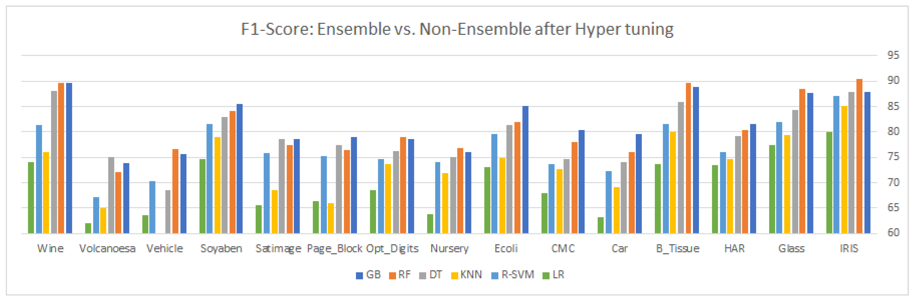
9. Results and Discussion

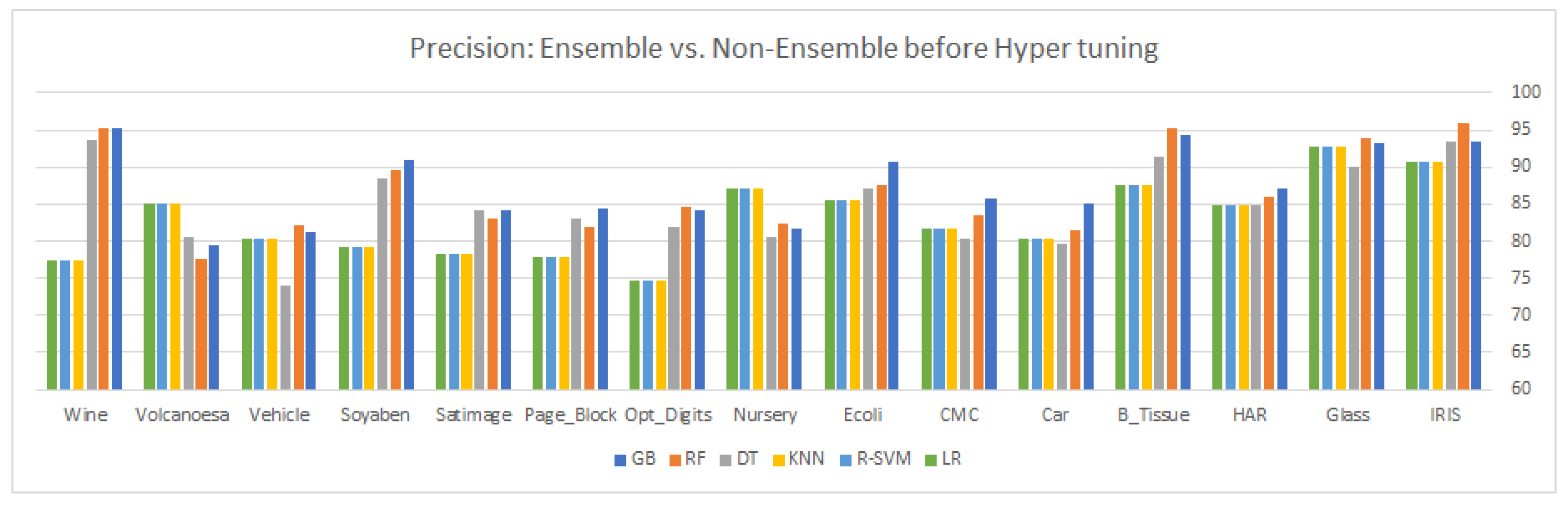
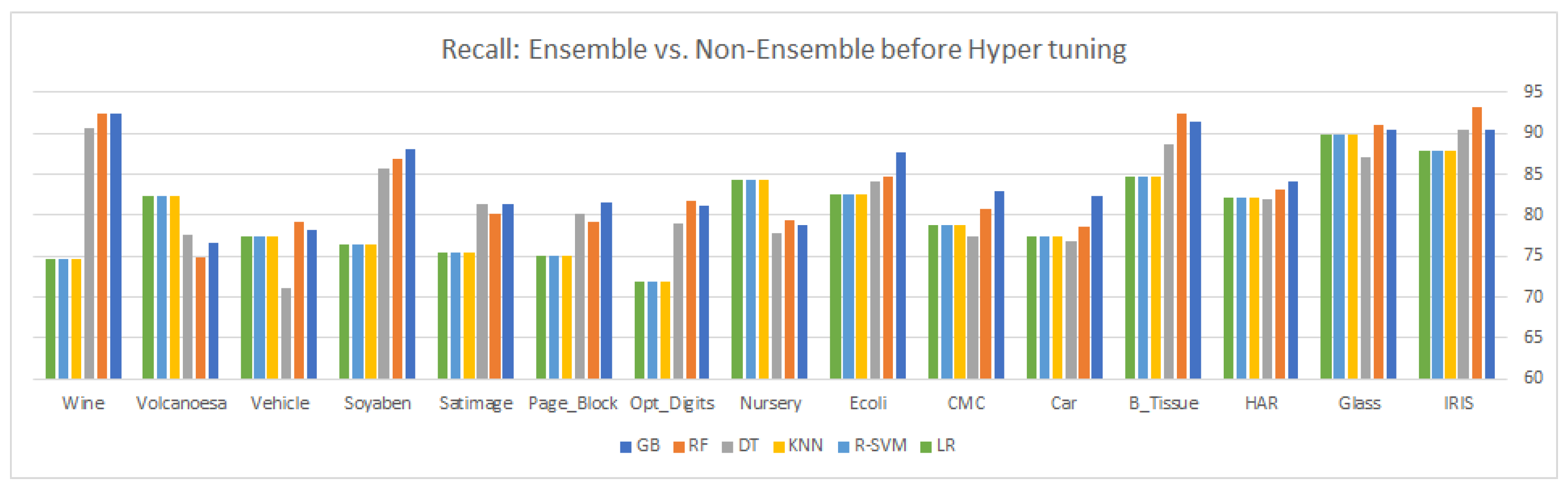
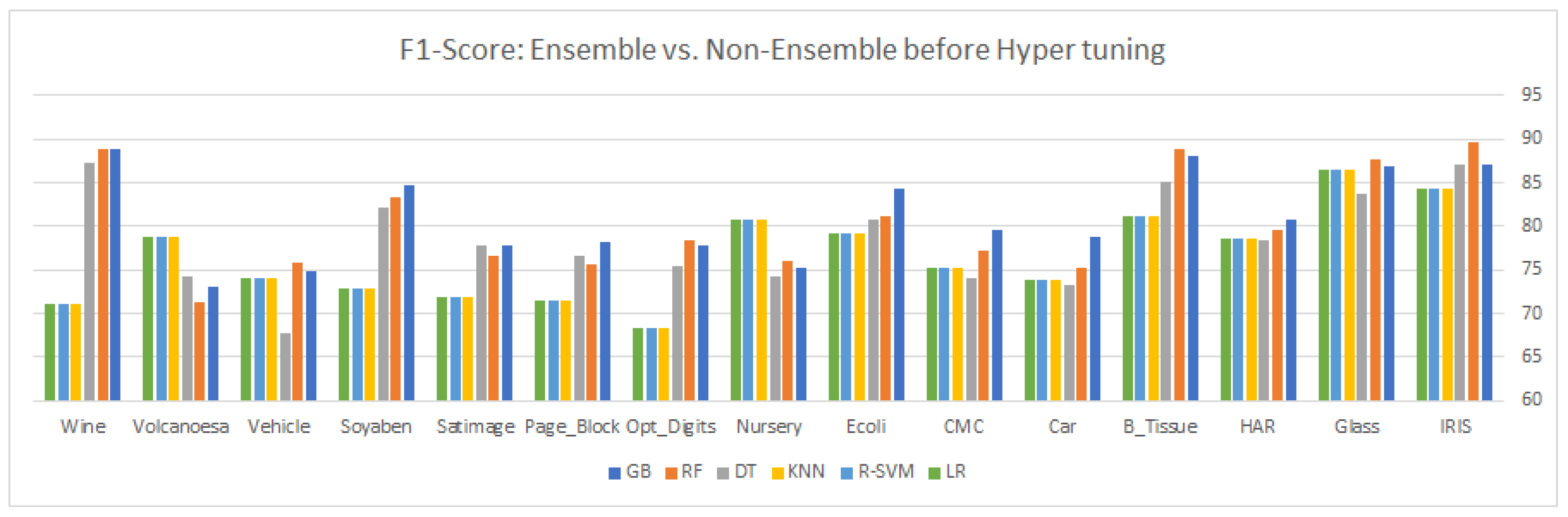
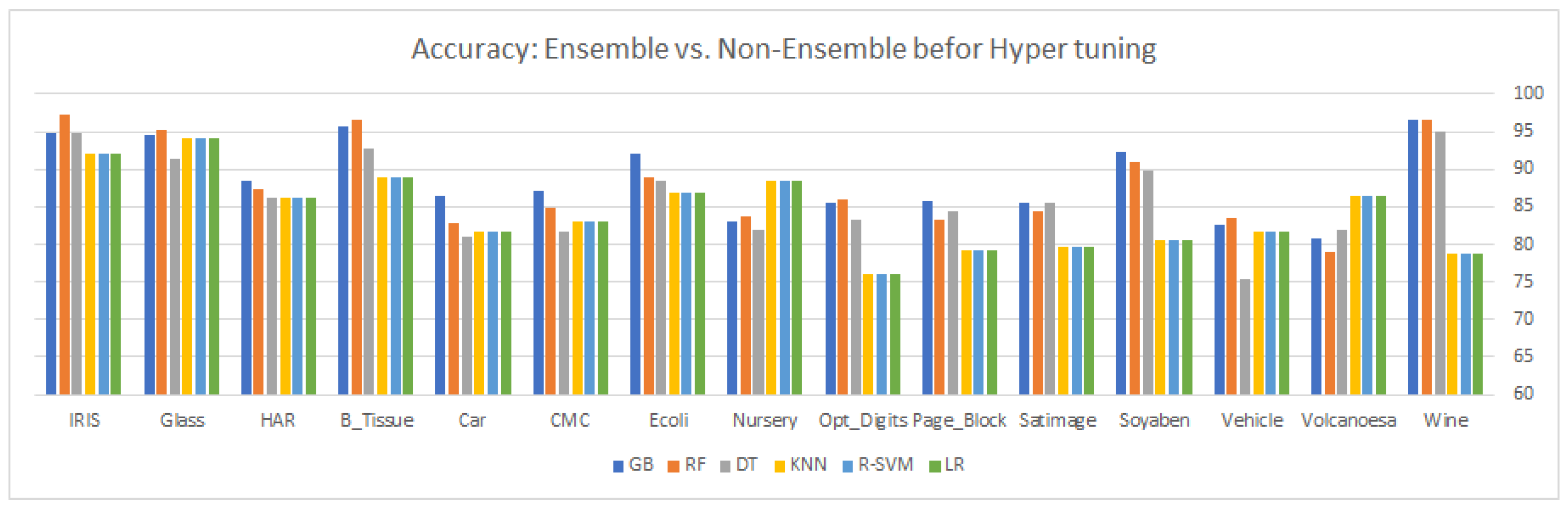
This article highlights three different aspects of ensemble and statistical classifiers depicted in Table 5, Table 6, Table 7, Table 8, Table 9 and Table 10 supplemented by the relevant graphical presentation in Figure 2, Figure 3, Figure 4, Figure 5, Figure 6, Figure 7, Figure 8, Figure 9, Figure 10, Figure 11, Figure 12 and Figure 13, respectively. This section carried out a detailed comparison to highlight the imbalance and overlapping nature of multi-class classification by applying traditional and ensemble approaches followed by some statistical analysis. Here, we applied different ensemble classifiers (GB, RF, and DT) and non-ensemble approaches (KNN, linear, kernel SVM, and NB) on 15 multi-class datasets. Each dataset consists of a different number of samples, features, and classes, i.e., the instances vary in the range of 150–12,960, while the number of features ranges from 4 to 65 and the number of classes varies between 3 and 20. 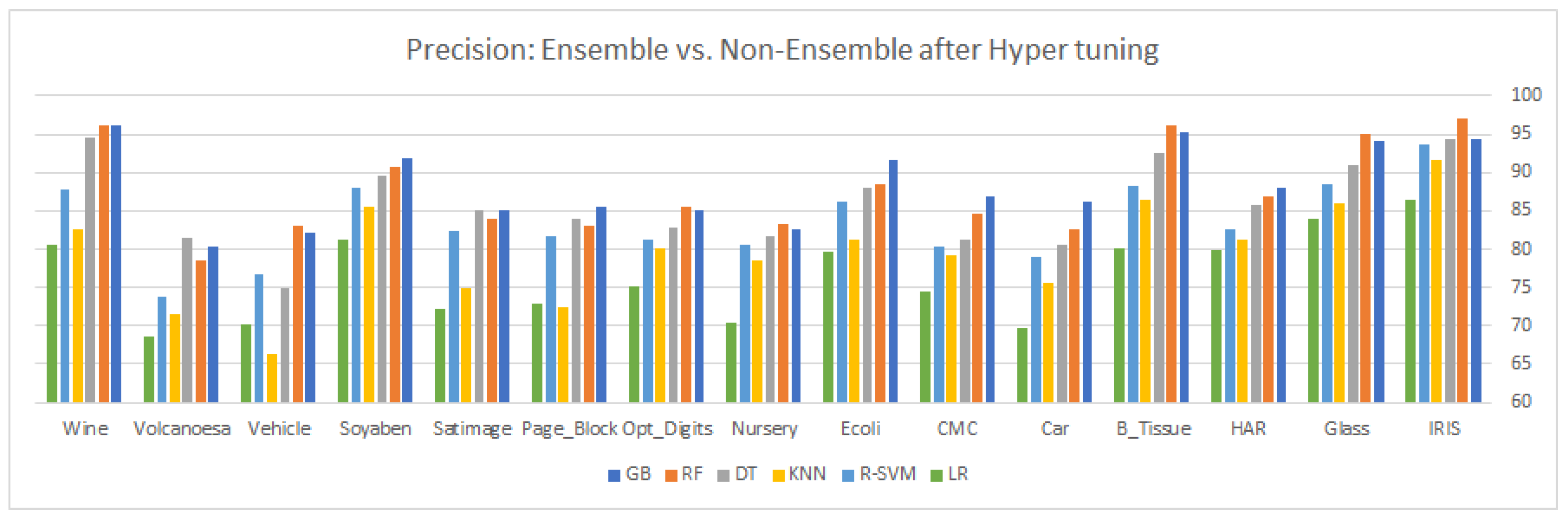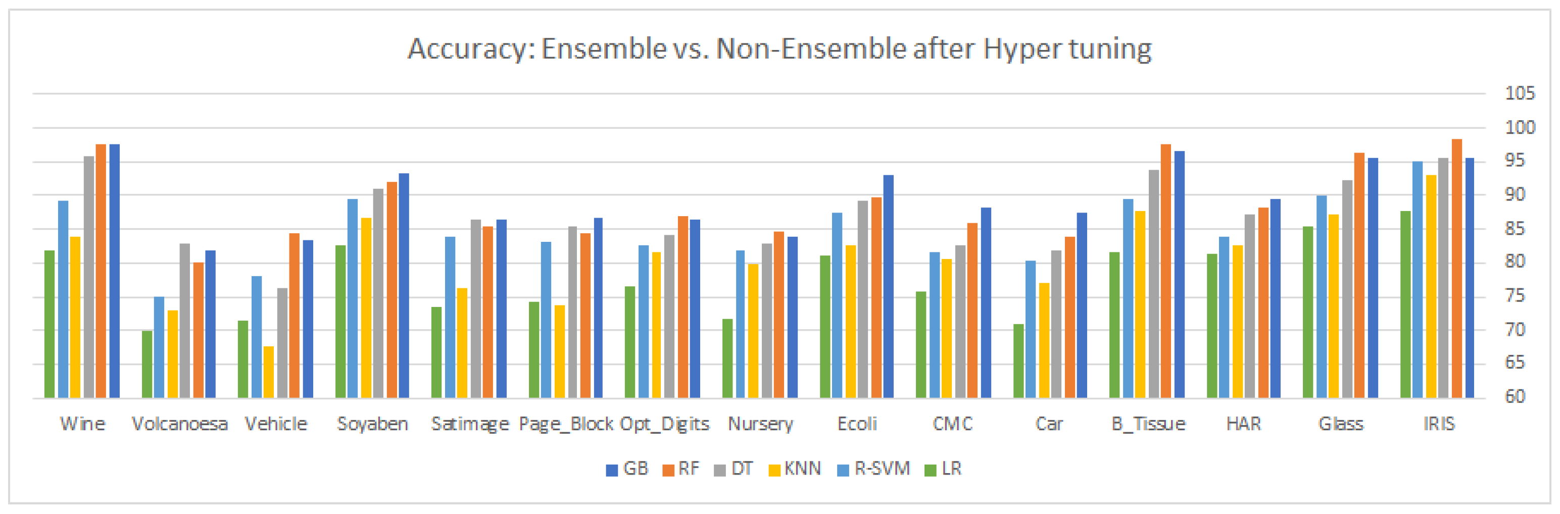Our results consist of three parts; first, we explore the six different classifiers on 15 multi-class datasets with default parameters and without synthetic overlapping, using confusion matrix values to gain insight into the different performance measures such as $accuracy$, $precision$, $recall$, and $f{1}_{score}$ as depicted in Table 5 and Table 6. In the second step, the six algorithms, namely GB, RF, DT, KNN, R-SVM, and LR are hyper-tuned (hyper-tuning the set of parameters) to improve the overall performance of the classification model, using 10-fold cross-validation in an exhaustive grid search technique experiment shown in Table 7 and Table 8.

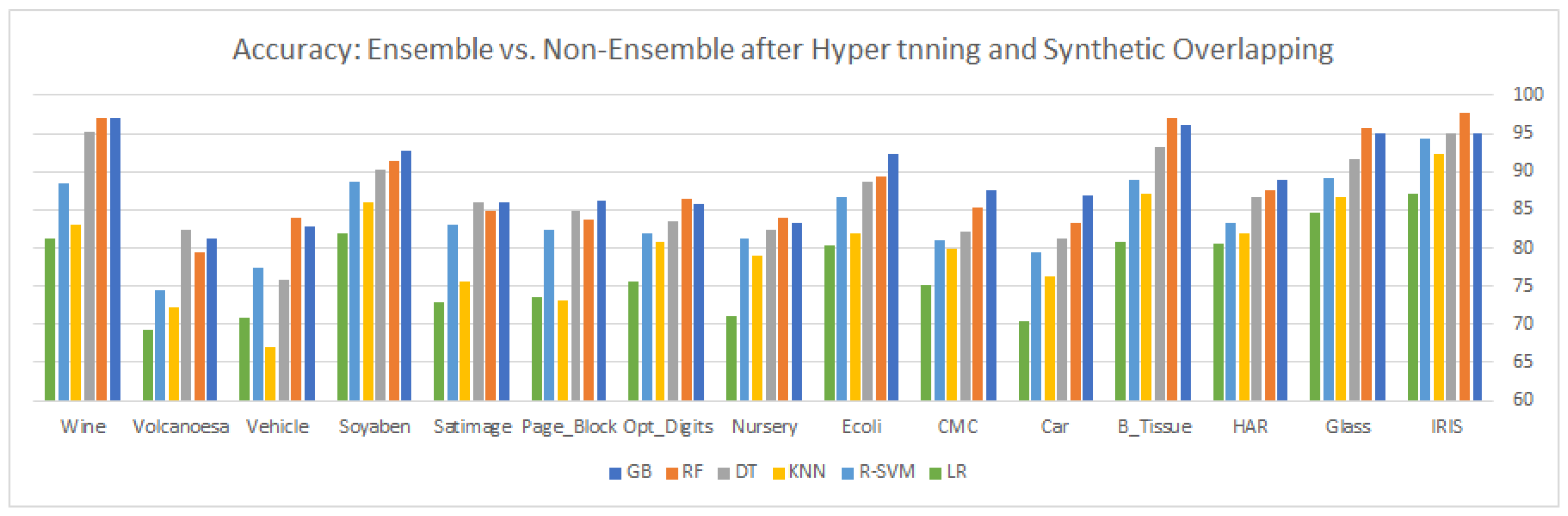
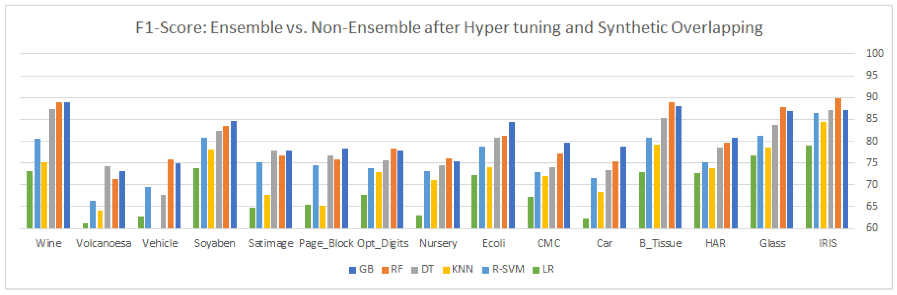
In the third part, the existing datasets (the majority class of each dataset) are synthetically overlapped by 20% of the original samples to glorify the impact of hyper-tuning the parameters, as shown in Table 9 and Table 10. After examining the results, we come up with these observations: gradient boosting an ensemble approach based on boosting shows remarkable performance in all categories (with and without hyper-tuning parameters for existing and synthetically overlapped datasets) for most of the multi-class imbalanced datasets. GB is an ensemble method, which combines many weak learners to produce a strong learner to deliver improved accuracy. A lower weight and a higher weight are assigned to the predicted outcome if it is correctly classified and misclassified, respectively. Each new tree is a fit on the reproduced subset of the original dataset during the boosting process. We tuned the tree-specific parameters during the hyper-tuning, boosting specific parameters and miscellaneous parameters. For some datasets in the experiment, all the classifiers $ensemble$ and $non-ensemble$ show power performance in terms of both accuracy and precision.

The reason for the power performance is the high variance and poor feature engineering makes it impossible for some algorithms to show a remarkable performance. Although boosting-based ensembles are prominent to control both bias and variance, sometimes with high variance and poor features, engineering them also fails to show a better performance. Along with the gradient boosting algorithm, random forest and decision tree also show some significance as compared to the other used classifier on most of the classifiers, particularly in the dataset with a greater number of features. The main reason for its significance is automatically reducing the number of features through its probabilistic entropy calculation approach. All three ensemble methods, GB, RF, and DT outperform the non-ensemble classifiers with both conventional hyper-tuned parameters for almost all the multi-class datasets. The error or misclassification rate can be dramatically reduced by averaging the component classifiers’ prediction report to produce an optimal final classification report both in a random forest and in the decision tree classifier. In the RFC, multiple trees are used in the ensemble to construct a sample drawn with a replacement from the training set. Moreover, a tree-based RFC ensemble selects a subset of features rather than using all the features of the data in the training set, resulting in the randomization of the tree. A decision tree break downs the classification process into multiple choices about each entry in our feature vector, starting with the root node and going downwards to the leaf where actual classification (prediction) is made. Unlike the traditional algorithm (black box learning algorithm), a decision tree is quite natural, as it visualizes and interprets the choices regarding how the tree is formed, and then follows a suitable path to the leaf node where actual predication or classification is performed. On the other hand, random forest, a collection of decision trees that vaccinate randomness at a certain level, makes it different from the decision tree classifier. The better performance of RF as compared to DT is because injecting randomness at two levels, in bootstrapping and during node splitting, causes a reduction in overfitting and resulting in an accurate model compared to the DT model. RF trains each distant DT on a bootstrapped sample drawn from the initial training dataset. Logistic regression is a linear classifier which can be applied to both linear and nonlinear problems, but as compared to ensemble approaches and SVM with an rbf kernel, the performance of LR is not good, as in other approaches. SVM in both versions (linear and kernel) is one of the most powerful models of machine learning with appropriate skills in separating the hyperplane on both the linear and nonlinear datasets. Sitting a hyperplane for a linear dataset is quite simple, by doing through the linear or rbf kernel, but for nonlinear data, the kernel tricks are used for sitting the hyperplane by projecting the data point in a higher dimension (in this N-dimension, the data points can easily be linearly separable). During the hyper-tuning process, when we set the decision function value to “one-versus-rest”, it decomposes the multi-class problem into several binary class problems, making it convenient for the SVM to find an optimal hyperplane, thus improving its overall model performance. To obtain the most successful results, proper feature engineering and feature scaling must be applied to the training dataset, as the LR model is greatly affected by different value ranges across dependent variables. On the majority of datasets, the poor performance of NB is because of the assumption that instances’ features are conditionally independent, but as we know in the case of the multi-class problem, features depend on each other, thus making this hypothesis wrong, which causes the degradation of the overall performance of the NB model. The basic working mechanism of the KNN model is based on the optimal value selected for k; whenever a new sample is subject to prediction, it simply examines the k-nearest neighbors from the training set, and the majority class among the k nearest neighbors are taken to be class for the test sample. Since the boundary regions of different classes in multi-class classification problems overlap with each other, it becomes difficult to examine the k-nearest neighbors from the training set.

As a final comment about the comparison, if we divide the classifiers between the ensemble and non-ensemble classifiers, the ensemble classifiers outperform the non-ensemble classifier on almost all the datasets with conventional and hyper-tuned parameters. Among the ensemble classifier, there is no constant winner for all the datasets, but overall gradient boosting beats all the classifiers for both categories. In non-ensemble methods, R-SVM shows a remarkable performance with the rbf kernel for both the conventional and tuned parameters, as SVM selects a small subset of training data from the original training data to construct the model. During the hyper-tuning process, when we set the decision function value to “one-versus-rest”, it decomposes the multi-class problem into several binary class problems, making it convenient for the SVM to find an optimal hyperplane, thus improving its overall model performance.

As we stated earlier in Section 9 about the synthetic generation of controlled overlapping samples in the existing dataset, if we look at the results of Table 5, Table 7 and Table 9, which show the accuracy and precision of the stated classifiers, respectively, the results of Table 5 are based on the scenarios in which we tested the ensemble and non-ensemble classifiers over the existing multi-class and overlapped dataset to highlight their performance. The result of Table 7 is based on the scenarios wherein we hyper-tuned the selected parameters of the classifiers using a 10-fold cross-validation and grid search technique, and then applied the selected classifiers to highlight the impact of parameters hyper-tuning over the multi-class and overlapped datasets. 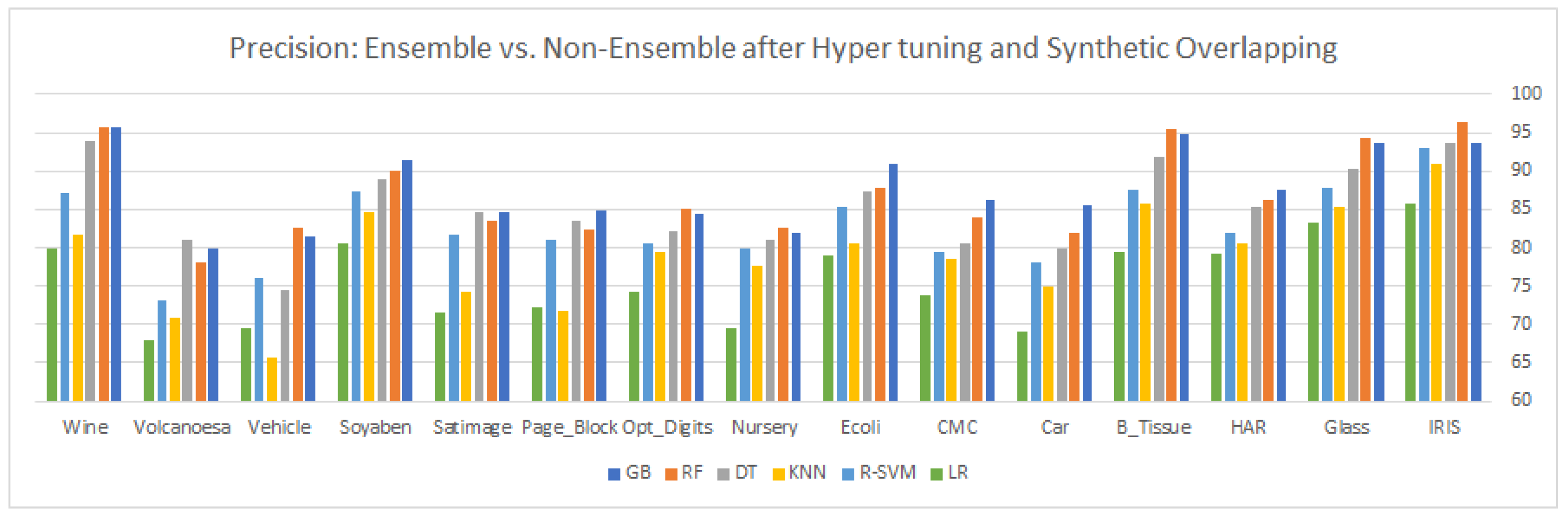After comparing both tables, it is clear that, after hyper-tuning the parameter set, the underlying classifier improved its performance, as discussed in Section 9. For the third scenario, we synthetically generated overlapping samples and 20% of these samples are inserted into the majority class of each dataset to increase the overlapping region of each dataset generation of synthetic samples is discussed in Section 10. After inserting the synthetic samples, the samples of majority and minority classes are more overlapped near the boundary region, resulting in a decrease in the visibility of the minority class. After compromising on the visibility of the minority class samples, the underlying classifier cannot predict the relevant target class effectively, hence decreasing the overall classifier performance. If we look at the results of Table 9, we se the accuracy and precision after the synthetic generation of samples and tuning of the parameters. 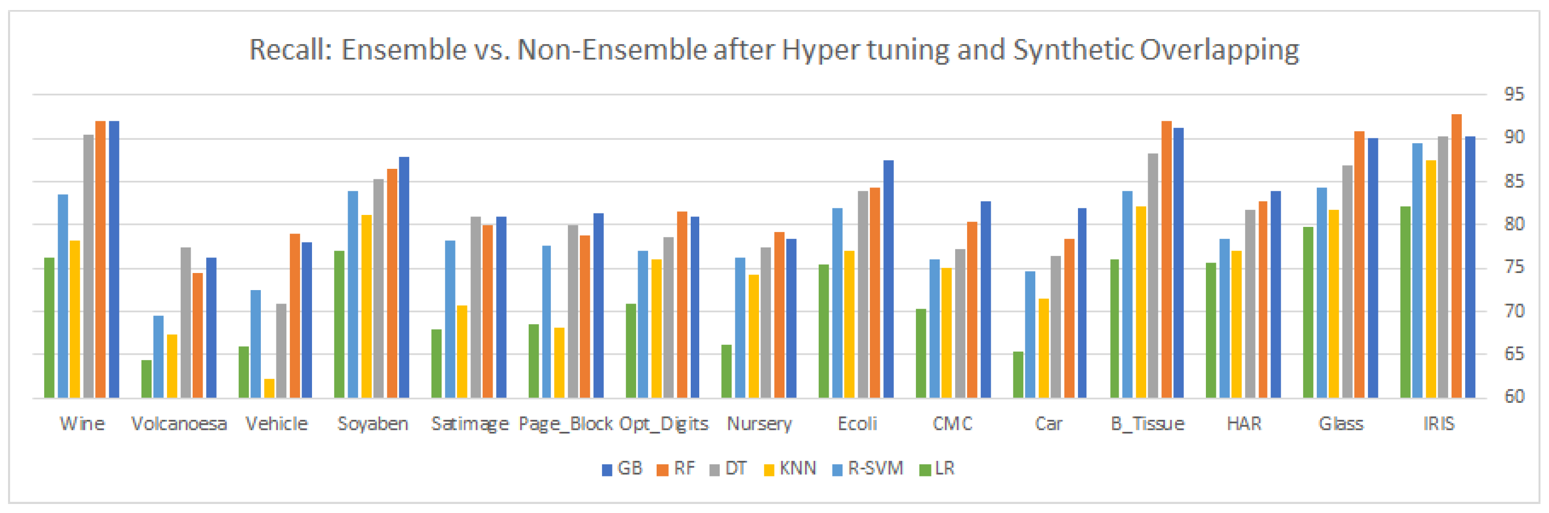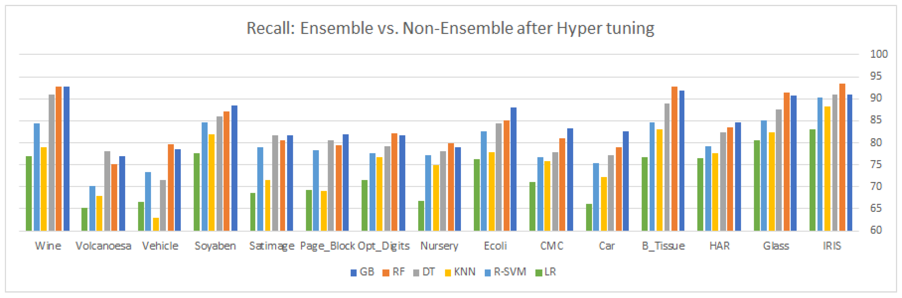If we compare the results in Table 9 with those in Table 5 and Table 7, there is a slight change in the classifier performance, even after the insertion of the synthetic samples in the majority of classes. The same justification is for recall and $f{1}_{score}$ as depicted in Table 6, Table 8 and Table 10.

10. Resultant Summary for Ensemble and Non-Ensemble Classifiers

As a final comment about the comparison, if we divide the classifiers into ensemble and non-ensemble (traditional) classifiers, the ensemble classifiers outperform the non-ensemble classifiers on almost all the datasets with conventional and hyper-tuned parameters.

Among the ensemble classifier, there is no constant winner for all the datasets, but overall, gradient boosting beats all the classifiers for both categories. In non-ensemble methods, R-SVM shows a remarkable performance with the rbf kernel for both the conventional and tuned parameters, as SVM selects a small subset of training data from the original training data to construct the model. The increasing size and dimensions of the problem space make it difficult for traditional or non-ensemble classifiers to correctly predict the unseen samples for multi-class classification data. The main reason behind the poor performance of traditional classifiers is the inability to tackle the high bias and variance. Despite so many machine-learning algorithms, the data to be processed need to be carefully examined, as every time, the data are biased, have high variance, or are sometimes noisy. When these unprocessed data (data with bias, variance, and noise) are subject to classification using the traditional algorithms, most of the time, we obtain a specialized model based on the training set, which yields low accuracy and loses of results. Due to the high bias, the underlying machine learning algorithm is unable to make a meaningful relation between the target variables (class labels) and the features, causing underfitting, which will reduce the overall performance of the classifiers on the testing set. On the other hand, high variance results in the random noise as a part of the training dataset, rather than the intended outputs, because the high variance in the underlying model tends to overfit on training data, resulting in a non-generalized model for the prediction. Compared to traditional classifiers, ensemble approaches try to reduce the variance and bias in the training data, resulting in a more robust and generalized model for the multi-class classification problem. The variance–bias tradeoff is a significant problem in almost all machine learning classifiers, particularly in the case of multi-class classification, where the boundaries of different classes are overlaps with each other’s, making it difficult to draw a clear hyperplane to separate the samples of multi classes. To correctly classify the unseen data during the validation process, ideally one can desire to choose such a machine-learning model, which apprehends the consistencies in its training dataset (effectively addressing the high variance and bias), also avoiding the under-fitting and over-fitting issues. Unfortunately, for most traditional classifiers, it is not an easy task to simultaneously reduce the high variance and bias. On the other hand, the ensemble approaches follow the ‘component-classifiers’ approach, wherein at each iteration, the misclassified sample (caused by high variance and bias) is again subject to the training subset. Ensemble classifiers are working in a parallel mode by assigning individual base learners to a ‘different-different machine’. In short, ensemble approaches are just like a ‘meta-algorithm’ by combining different learning models into a more robust single model to improve the overall performance of the underlying model. The high bias in the training data was reduced via the boosting approach and the high variance was reduced via the bagging approach. All the acronyms used in this article are defined in

Table 12. Acronyms and their definitions.

Acronym	Description
KNN	k-Nearest Neighbor
NB	Naive Bayes
ANN	Artificial Neural Network
DT	Decision Tree
SVM	Support Vector Machine
LR	Logistic Regression (LR)
G-mean	Geometric Mean
F1-Score	F-Measure
AUC	Area under Curve
TBWRSVM	Twin Bounded Weighted Relaxed Support Vector Machines
WRSVM	Weighted Relaxed Support Vector Machine
DES-MI	Dynamic Ensemble Selection for Multi-Class Imbalanced the Dataset
GSVD	Generalized Singular Value Decomposition
MDO	Mahalanobis Distance-based Oversampling
EC	Evolutionary Computation
SaFWA	Self-Adaptive Fireworks Algorithm
CSGSs	Candidate Solution Generation Strategies
k-SMOTE	k-Means Clustering
split	Minimum-Sample-Split
OVO	One-versus-One Decomposition Strategies
OVR	One-versus-Rest Decomposition Strategies
solver, newton-cg, sag, and lbfgs	Multinomial values
RSM	Response Surface Methodology
MAE	Mean Absolute Error
labelencoder.fit	Label Encoding Scheme
MDS	Multiclass Dataset

.

11. Conclusions

In this paper, we applied six different algorithms (ensemble and non-ensemble) on 15 multi-class datasets with default parameters, and then compared the results with hyper-tuned parameters. The results highlight the significant improvement in the categories of the algorithm after both hyper-tuning a set of parameters and performing an exhaustive grid search technique. However, ensemble approaches outperform the non-ensemble approaches for the majority of multi-class classification datasets. Before applying classification algorithms to the stated imbalanced dataset, we did not apply any data-level approach to balance the dataset. Similarly, after synthetically overlapping the existing datasets, ensemble classifiers show the same results compared to statistical approaches. The results can be further improved if we augment the data level approaches with the ensemble and non-ensemble approaches.

As a future direction, if we perform proper feature engineering on the multi-class imbalanced dataset, the results will surely improve. A combination of ensemble classifiers with a cost-sensitive approach (assigning misclassification cost) can significantly improve the overall performance of the different classifiers. One-class learners, within-class imbalance, small disjuncts, feature selection, stacked ensembles, sophisticated over-sampling techniques, and within-class imbalance are among the research gaps that need to be specially addressed in a future study.