
MEMD-Based Hybrid Modal Identification for High-Rise Structures with Multi-Sensor Vibration Measurements


Abstract
:1. Introduction
2. Methodology
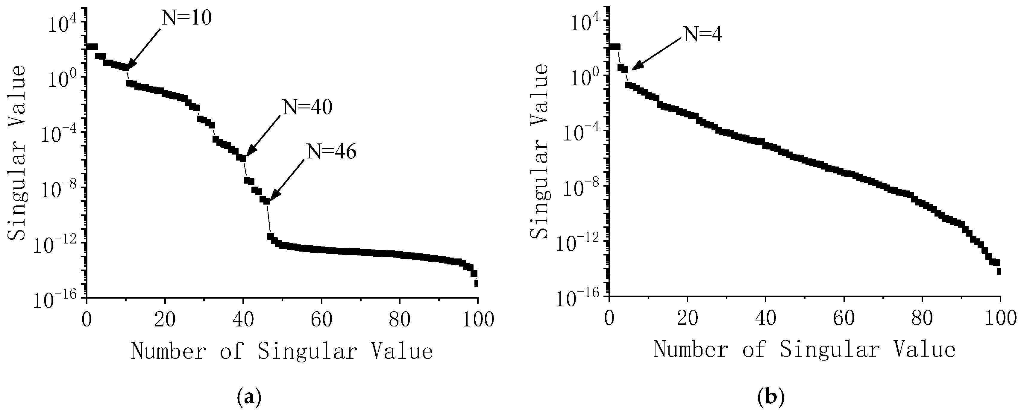
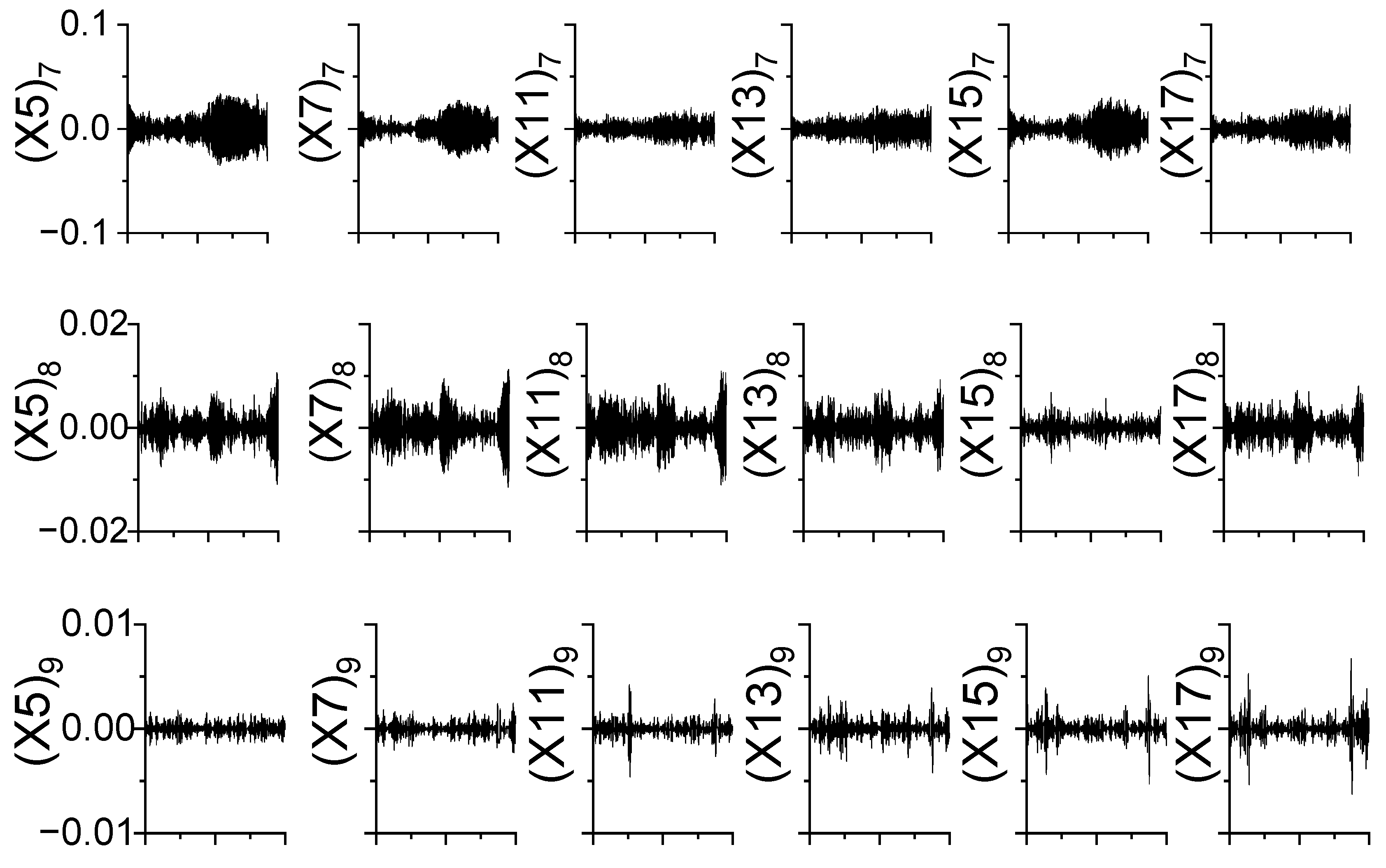
2.1. MEMD
- (1)
- Generate n-point low-discrepancy Hammersley sequences to sample on an () dimensional sphere.
- (2)
- Project the original signal along each directional vector , where is the number of directional vectors, denoted as of each vector.
- (3)
- Pick up the time instants of the maximums of every projection .
- (4)
- Interpolate to generate the multiple envelope by a spline.
- (5)
- Calculate the mean curve for all envelopes
- (6)
- Subtract the mean curve from the original signal . If the detail satisfies the stoppage criterion, it can be regarded as the first IMF, otherwise, repeat step 2 to step 5 to regenerate . Then, apply the above steps with to obtain other IMFs.
2.2. Memd-Based Identification Methods
2.2.1. MEMD-Based SSI (MSSI) Method
2.2.2. MEMD-Based FBFFT (MFBFFT) Method
3. Case Study
3.1. Numerical 5-Storey Frame Structure
3.2. Shaking Table Modal Test
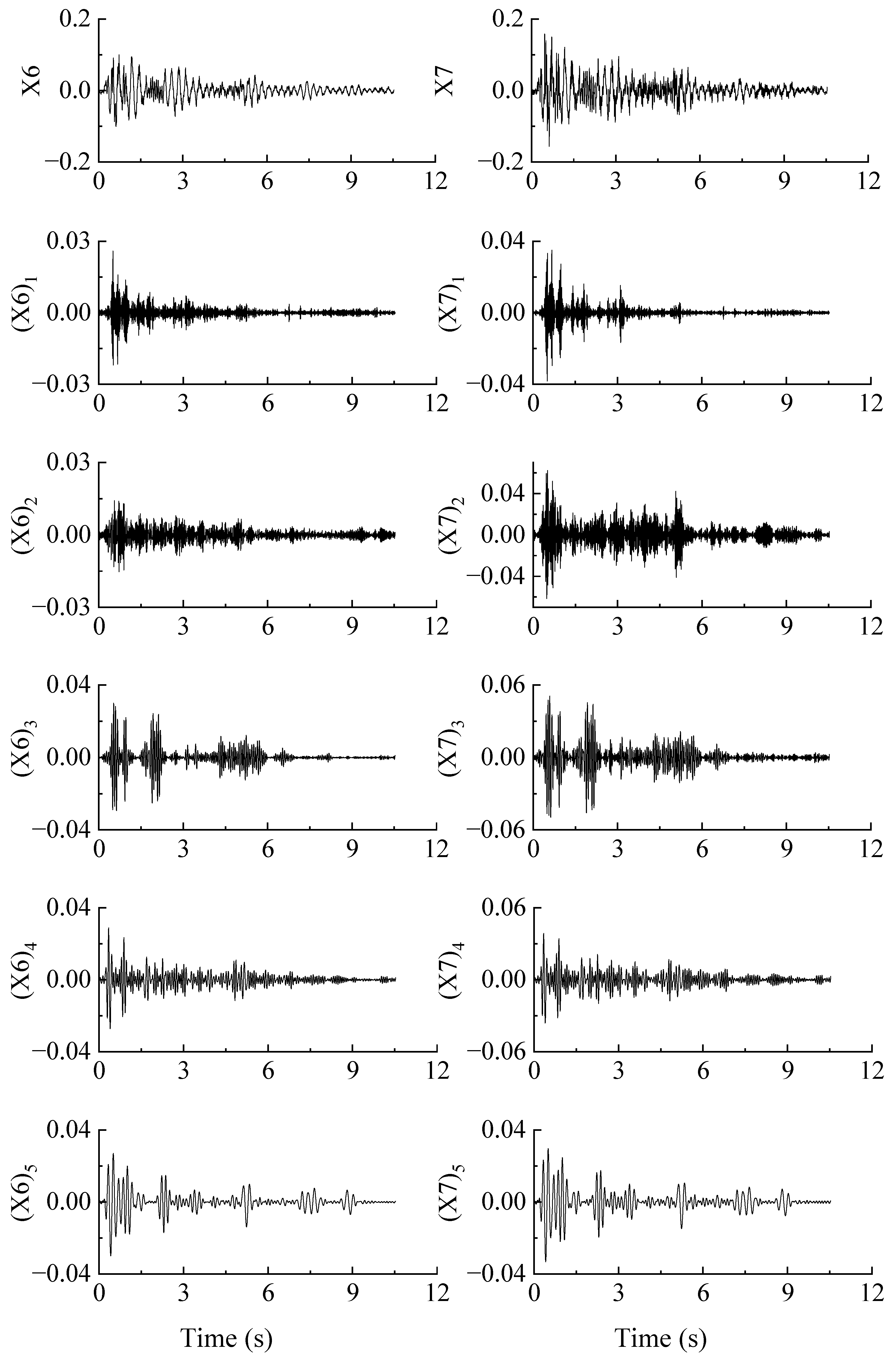
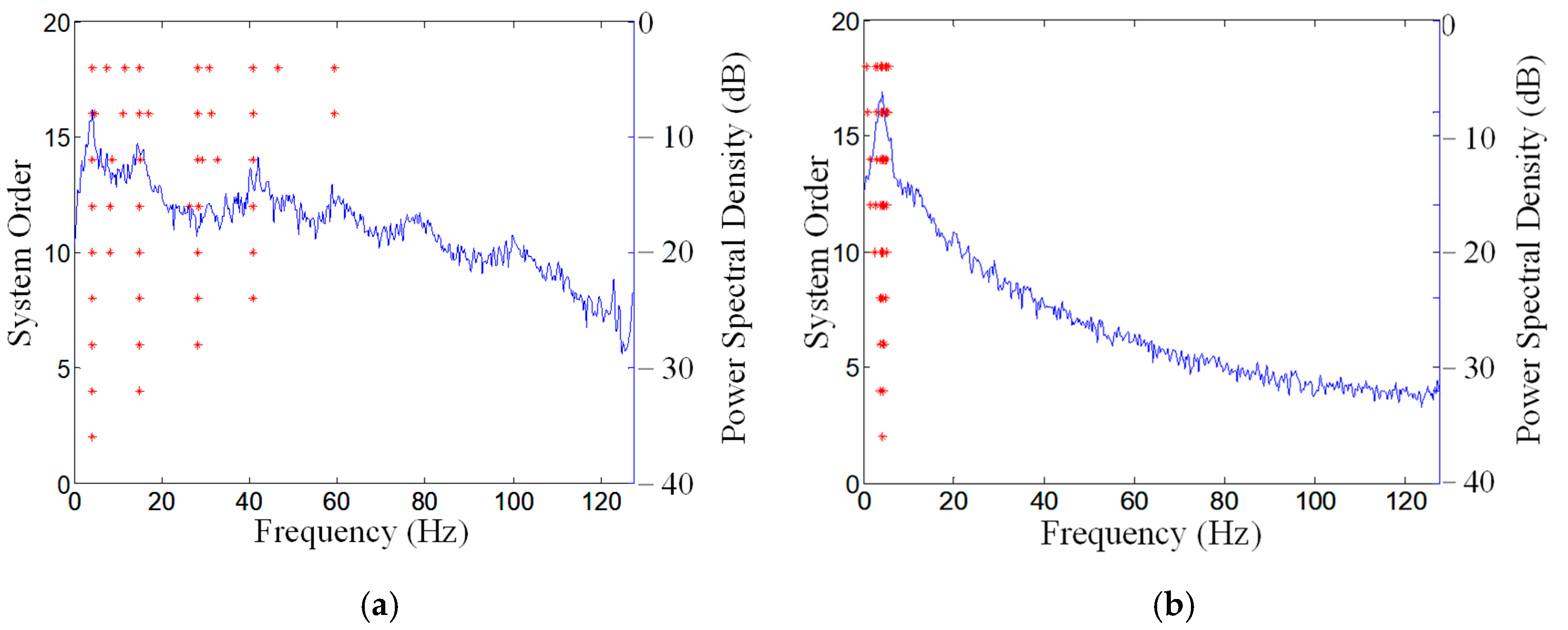
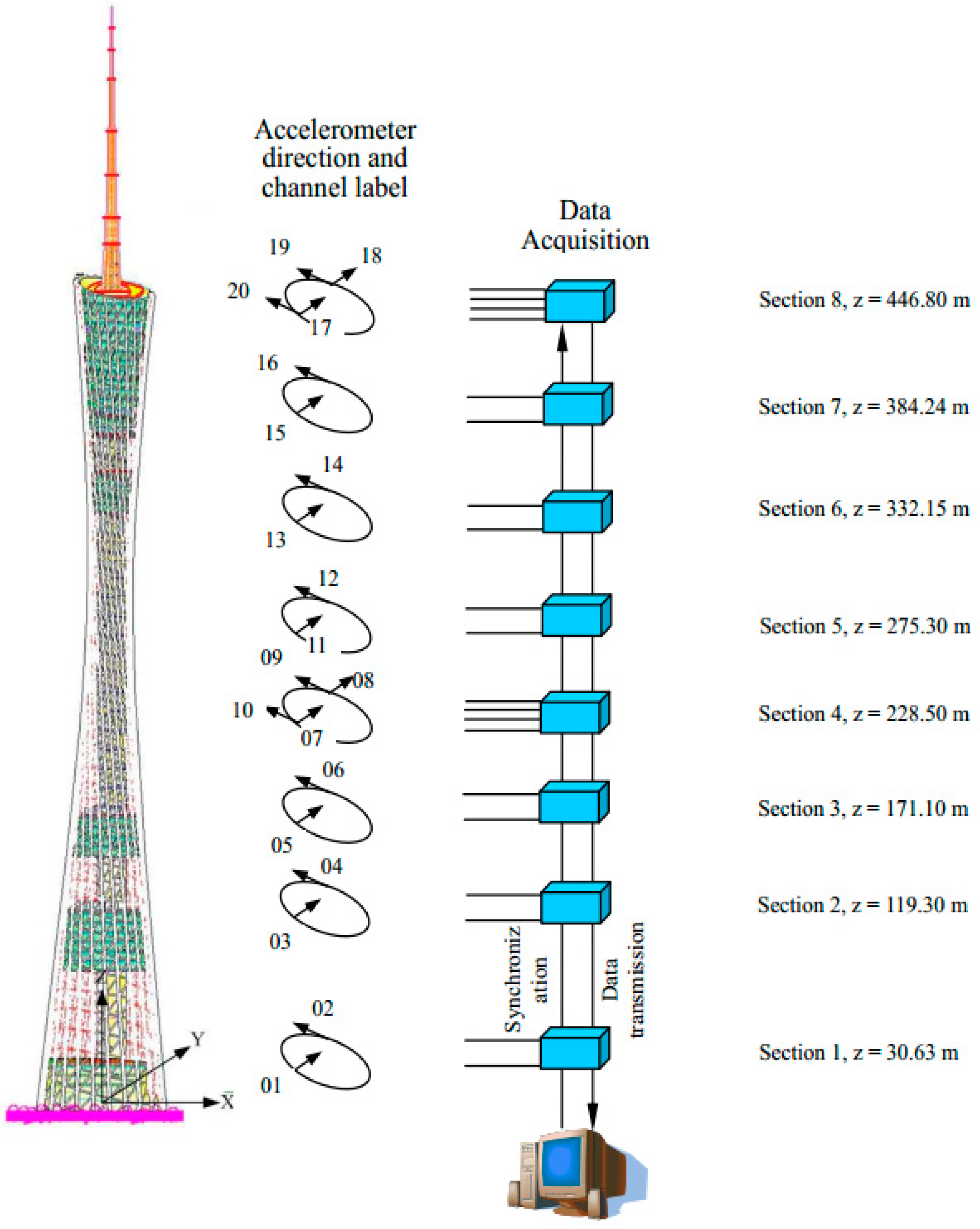
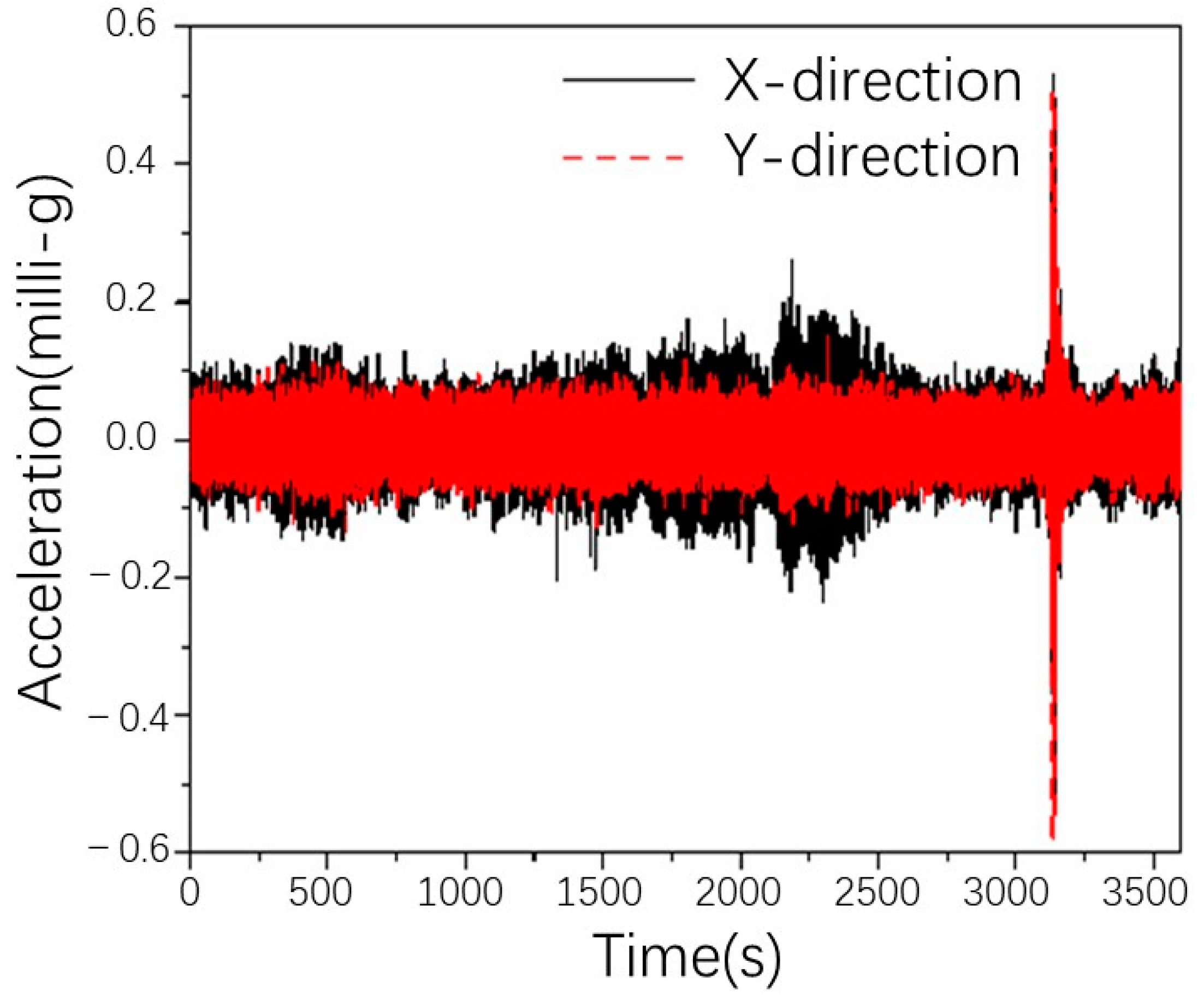
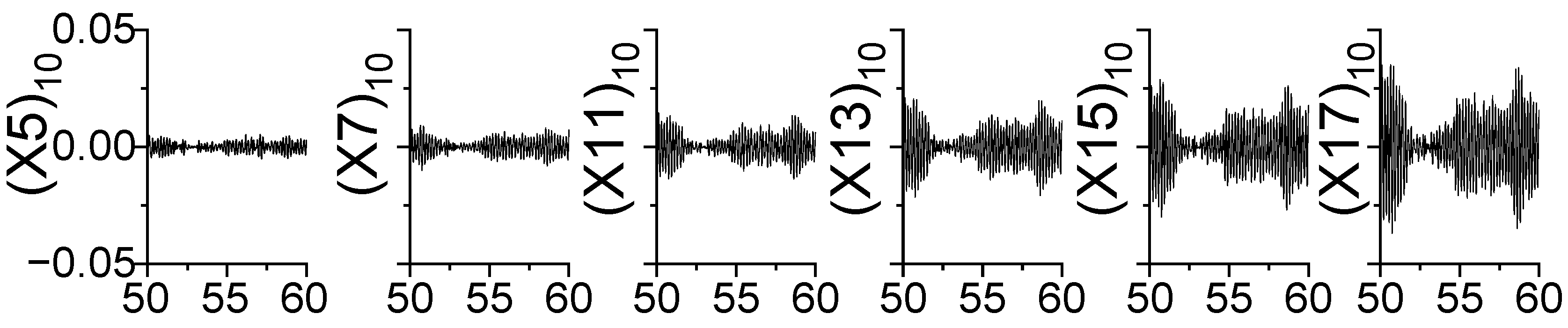
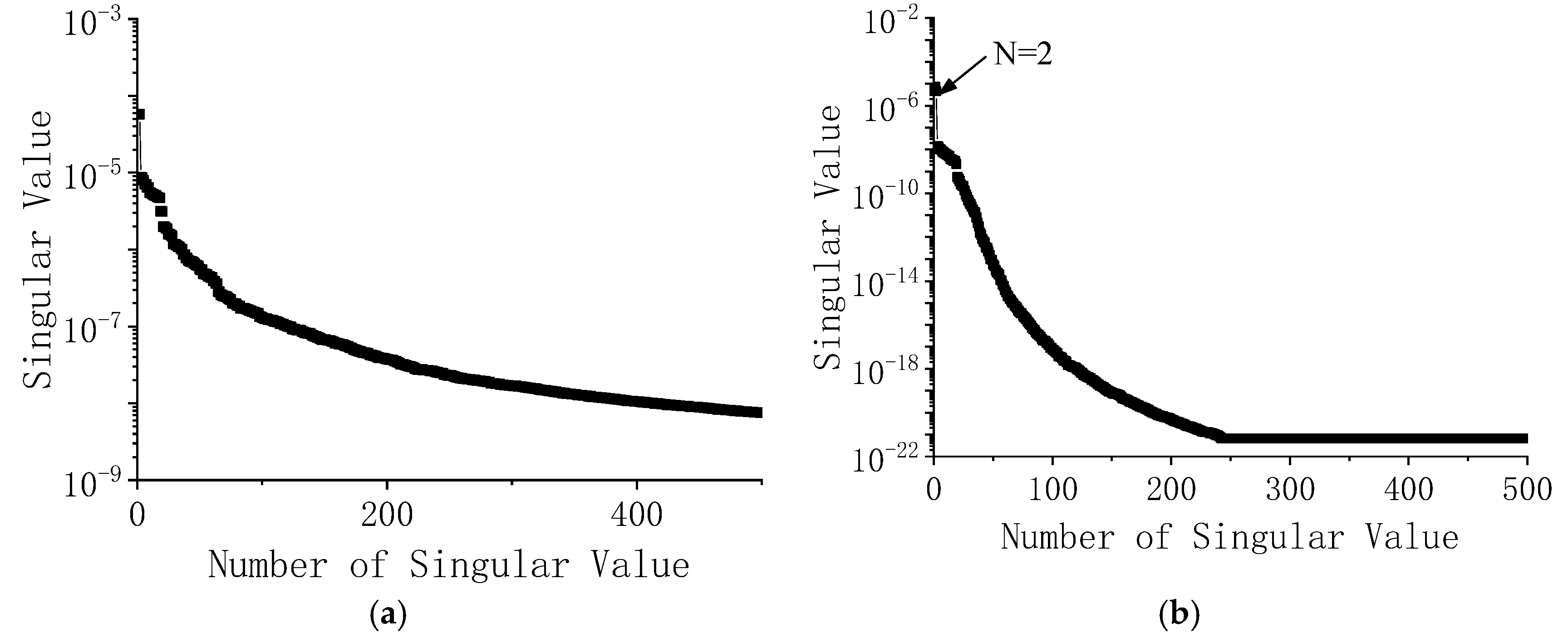
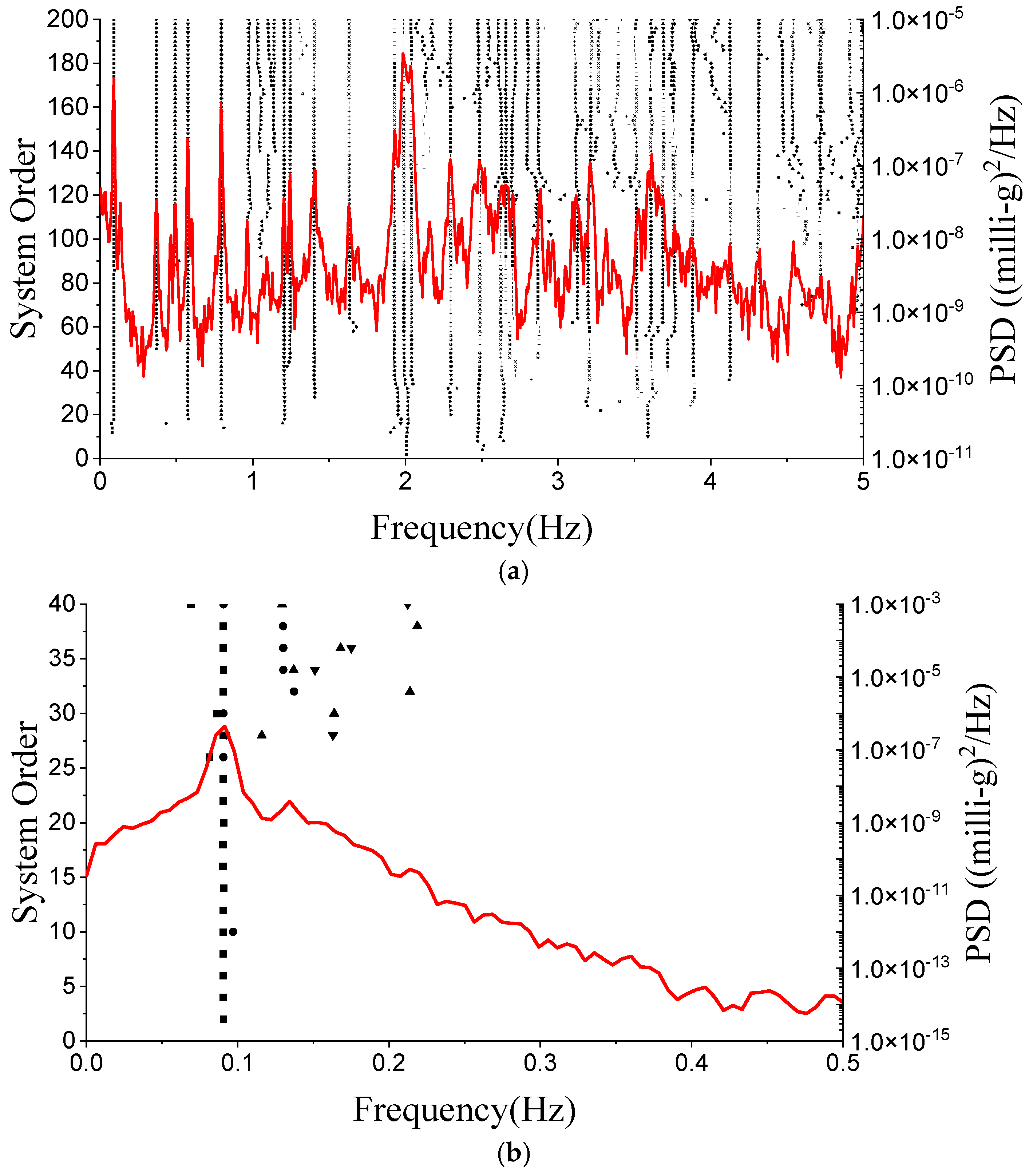
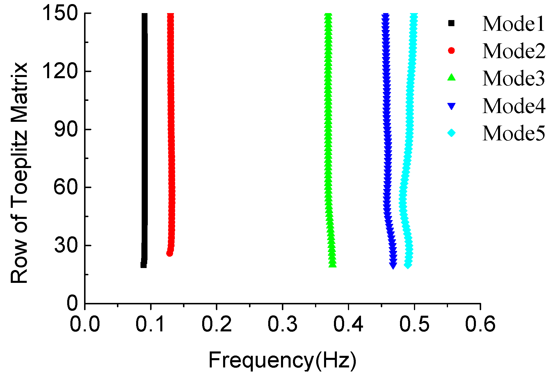
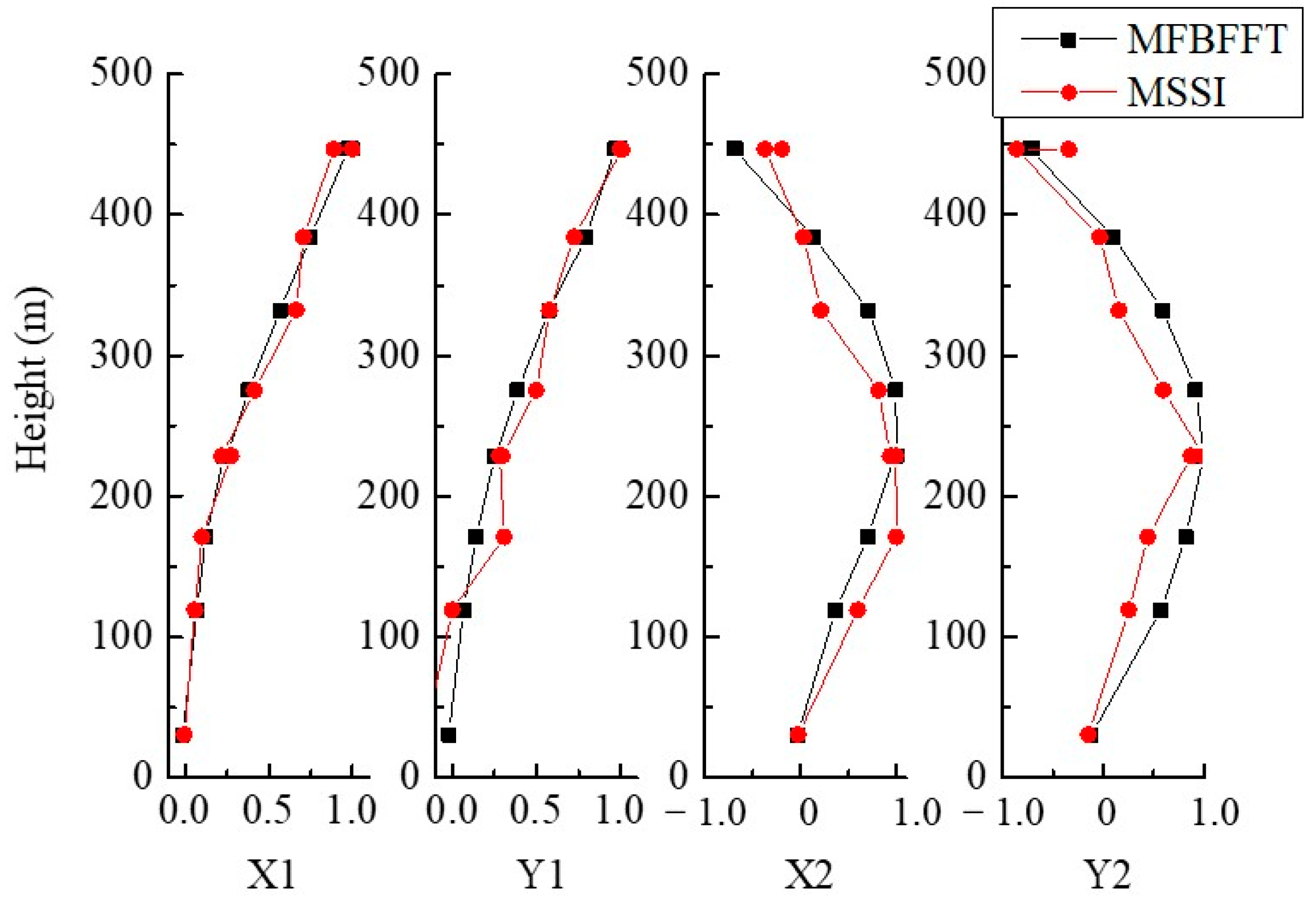
4. Full-Scale Measurement of the Canton Tower
5. Discussion
6. Conclusions
Author Contributions
Funding
Institutional Review Board Statement
Informed Consent Statement
Data Availability Statement
Conflicts of Interest
References
- Brincker, R.; Ventura, C.E.; Andersen, P. Damping estimation by Frequency Domain Decomposition. In Proceedings of the IMAC 19: A Conference on Structural Dynamics, Hyatt Orlando, Kissimmee, FL, USA, 5–8 February 2001. [Google Scholar]
- Brincker, R.; Zhang, L.; Andersen, P. Modal identification of output-only systems using frequency domain decomposition. Smart Mater. Struct. 2001, 10, 441–445. [Google Scholar]
- James, G.H.I.; Carne, T.G.; Lauffer, J.P. The natural excitation technique (NExT) for modal parameter extraction from operating wind turbines. Int. J. Anal. Exp. Modal Anal. 1993, 93, 260–277. [Google Scholar]
- Abazarsa, F.; Nateghi, F.; Ghahari, S.F.; Taciroglu, E. Extended blind modal identification technique for nonstationary excitations and its verification and validation. J. Eng. Mech. 2016, 142, 04015078. [Google Scholar]
- Ghahari, S.F.; Abazarsa, F.; Ghannad, M.A.; Celebi, M.; Taciroglu, E. Blind modal identification of structures from spatially sparse seismic response signals. Struct. Control Health Monit. 2014, 21, 649–674. [Google Scholar]
- Chiang, D.Y.; Lin, C.S. Identification of modal parameters from nonstationary ambient vibration data using the channel-expansion technique. J. Mech. Sci. Technol. 2011, 25, 1307–1315. [Google Scholar]
- Huang, N.E.; Shen, Z.; Long, S.R.; Wu, M.C.; Shih, H.H.; Zheng, Q. The empirical mode decomposition and the Hilbert spectrum for nonlinear and non-stationary time series analysis. Proc. R. Soc. A Math. Phys. Eng. Sci. 1998, 454, 903–995. [Google Scholar]
- Huang, N.E.; Wu, M.L.C.; Long, S.R.; Qu, W.; Gloersen, P.; Fan, K.L. A confidence limit for the empirical mode decomposition and Hilbert spectral analysis. Proc. R. Soc. London. Ser. A Math. Phys. Eng. Sci. 2003, 459, 2317–2345. [Google Scholar]
- Yang, J.N.; Lei, Y.; Lin, S.; Huang, N. Identification of natural frequencies and dampings of in situ tall buildings using ambient wind vibration data. J. Eng. Mech. 2004, 130, 570–577. [Google Scholar]
- He, X.H.; Hua, X.G.; Chen, Z.Q.; Huang, F.L. EMD-based random decrement technique for modal parameter identification of an existing railway bridge. Eng. Struct. 2011, 33, 1348–1356. [Google Scholar]
- Yu, D.J.; Ren, W.X. EMD-based stochastic subspace identification of structures from operational vibration measurements. Eng. Struct. 2005, 27, 1741–1751. [Google Scholar]
- Han, J.; Zheng, P.; Wang, H. Structural modal parameter identification and damage diagnosis based on Hilbert-Huang transform. Earthq. Eng. Eng. Vib. 2014, 13, 101–111. [Google Scholar]
- Rilling, G.; Flandrin, P.; Gonçalves, P.; Lilly, J.M. Bivariate empirical mode decomposition. IEEE Signal Processing Lett. 2007, 14, 936–939. [Google Scholar]
- Rehman, N.; Mandic, D.P. Empirical mode decomposition for trivariate signals. IEEE Trans. Signal Processing 2010, 58, 1059–1068. [Google Scholar]
- Huang, G.; Su, Y.; Kareem, A.; Liao, H. Time-frequency analysis of nonstationary process based on multivariate empirical mode decomposition. J. Eng. Mech. 2015, 142, 04015065. [Google Scholar]
- Sadhu, A. An integrated multivariate empirical mode decomposition method towards modal identification of structures. J. Vib. Control 2017, 23, 2727–2741. [Google Scholar]
- Barbosh, M.; Sadhu, A.; Vogrig, M. Multisensor-based hybrid empirical mode decomposition method towards system identification of structures. Struct. Control. Health Monit. 2018, 25, e2147.1–e2147.21. [Google Scholar]
- Aruljayachandran, M.; Kareem, A.; Kwon, D.K. Identification of vortex-induced vibration of tall building pinnacle using cluster analysis for fatigue evaluation: Application to burj khalifa. J. Struct. Eng. 2020, 146, 04020234. [Google Scholar]
- Zhang, L.; Hu, X.; Xie, Z. Identification method and application of aerodynamic damping characteristics of super high-rise buildings under narrow-band excitation. J. Wind Eng. Ind. Aerodyn. 2019, 189, 173–185. [Google Scholar]
- Au, S.K.; Brownjohn, J.; Mottershead, J.E. Quantifying and managing uncertainty in operational modal analysis. Mech. Syst. Signal Processing 2017, 102, 139–157. [Google Scholar]
- Rehman, N.; Mandic, D.P. Multivariate empirical mode decomposition. Proc. R. Soc. A 2010, 466, 1291–1302. [Google Scholar]
- Dalal, I.L.; Stefan, D.; Harwayne-Gidansky, J. Low discrepancy sequences for Monte Carlo simulations on reconfigurable platforms. In Proceedings of the 2008 International Conference on Application-Specific Systems, Architectures and Processors, Leuven, Belgium, 2–4 July 2008. [Google Scholar]
- Komaty, A.; Boudraa, A.O.; Flandrin, P.; Amblard, P.O.; Astolfi, J.A. On the Behavior of MEMD in Presence of Multivariate Fractional Gaussian Noise. IEEE Trans. Signal Processing 2021, 69, 2676–2688. [Google Scholar]
- Xia, Y.; Zhang, B.; Pei, W.; Mandic, D.P. Bidimensional Multivariate Empirical Mode Decomposition with Applications in Multi-Scale Image Fusion. IEEE Access 2019, 7, 114261–114270. [Google Scholar]
- Lang, X.; Zheng, Q.; Zhang, Z.; Lu, S.; Xie, L.; Horch, A.; Su, H. Fast multivariate empirical mode decomposition. IEEE Access 2018, 6, 65521–65538. [Google Scholar]
- Peeters, B.; Roeck, G.D. Reference-based stochastic subspace identification for output-only modal analysis. Mech. Syst. Signal Processing 1999, 13, 855–878. [Google Scholar]
- Peeters, B.; De Roeck, G. Reference based stochastic subspace identification in civil engineering. Inverse Probl. Eng. 2000, 8, 47–74. [Google Scholar]
- Van Overschee, P.; De Moor, B. Subspace Identification for Linear Systems: Theory, Implementation and Applications; Kluwer Academic Publishers: Dordrecht, The Netherlands, 1996. [Google Scholar]
- Loh, C.H.; Liu, Y.C.; Ni, Y.Q. SSA-based stochastic subspace identification of structures from output-only vibration measurements. Smart Struct. Syst. 2012, 10, 331–351. [Google Scholar]
- Reynders, E.; Pintelon, R.; Roeck, G.D. Uncertainty bounds on modal parameters obtained from stochastic subspace identification. Mech. Syst. Signal Processing 2008, 22, 948–969. [Google Scholar]
- Zini, G.; Betti, M.; Bartoli, G. A quality-based automated procedure for operational modal analysis. Mech. Syst. Signal Processing 2022, 164, 108173. [Google Scholar]
- Priori, C.; Angelis, M.D.; Betti, R. On the selection of user-defined parameters in data-driven stochastic subspace identification. Mech. Syst. Signal Processing 2018, 100, 501–523. [Google Scholar]
- Yuen, K.V. Structural Modal Identification Using Ambient Dynamic Data. Master’s Thesis, Hong Kong University of Science and Technology, Hong Kong, 1999. [Google Scholar]
- Au, S.K.; Ping, T. Full-scale validation of dynamic wind load on a super-tall building under strong wind. J. Struct. Eng. 2012, 138, 1161–1172. [Google Scholar]
- Yuen, K.V.; Katafygiotis, L.S.; Beck, J.L. Spectral density estimation of stochastic vector processes. Probabilistic Eng. Mech. 2002, 17, 265–272. [Google Scholar]
- Korwar, R.M. On characterizations of distributions by mean absolute deviation and variance bounds. Ann. Inst. Stat. Math. 1991, 43, 287–295. [Google Scholar]
- Water, T.P. Finite Element Model Updating Using Measured Frequency Response Functions. Ph.D. Thesis, University of Bristol, Bristol, UK, 1995. [Google Scholar]
- Li, Q.S.; Wu, J.R. Correlation of dynamic characteristic of a super tall building from full-scale measurements and numerical analysis with various finite element models. Earthq. Eng. Struct. Dyn. 2004, 33, 1311–1336. [Google Scholar]
- Lu, X.L.; Li, P.Z.; Chen, Y.Q. Complete Data of Shaking Table Test on a 12-Story Reinforced Concrete Frame Model; State Key Laboratory of Disaster Reduction in Civil Engineering, Tongji University: Shanghai, China, 2004. [Google Scholar]
- Lu, X.L.; Zhang, J.; Lu, W.S. Seismic behavior of vertically mixed structures with upper steel and lower concrete components. J. Build. Struct. 2011, 32, 20–26. (In Chinese) [Google Scholar]
- Ni, Y.Q.; Xia, Y.; Liao, W.Y.; Ko, J.M. Technology innovation in developing the structural health monitoring system for Guangzhou new TV tower. Struct. Control Health Monit. 2009, 16, 73–98. [Google Scholar]
- Ni, Y.Q.; Xia, Y.; Lin, W.; Chen, W.H.; Ko, J.M. SHM benchmark for high-rise structures: A reduced-order finite element model and field measurement data. Smart Struct. Syst. 2012, 10, 411–426. [Google Scholar]
- Guo, Y.L.; Kareem, A.; Ni, Y.Q.; Liao, W.Y. Performance evaluation of canton tower under winds based on full-scale data. J. Wind. Eng. Ind. Aerodyn. 2012, 104–106, 116–128. [Google Scholar]
- Li, H.; Liu, J.K.; Chen, W.H.; Lu, Z.R.; Xia, Y.; Ni, Y.Q. Analysis of dynamic characteristics of the Canton Tower under different earthquakes. Adv. Struct. Eng. 2015, 18, 1087–1100. [Google Scholar]


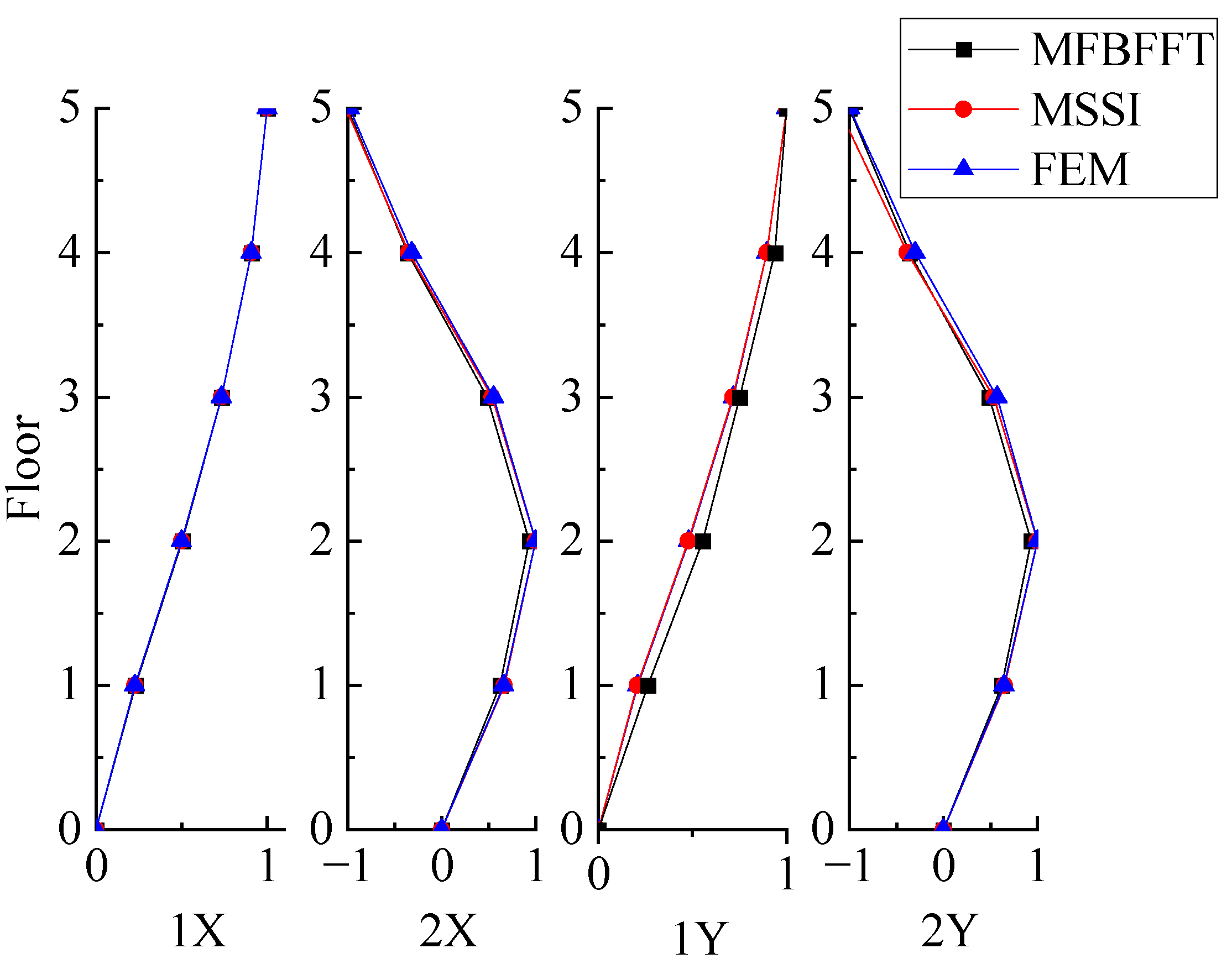
| Mode | FEM | PP | HHT | FBFFT | MFBFFT | SSI | MSSI | ||
|---|---|---|---|---|---|---|---|---|---|
| MPV | COV | MPV | COV | ||||||
| 1X | 3.7821 | 3.7840 | 3.8415 | 3.7897 | 0.12% | 3.7859 | 0.12% | 3.7836 | 3.7857 |
| 2X | 11.3600 | 11.1816 | 11.2436 | 11.3420 | 0.10% | 11.3021 | 0.11% | 11.3472 | 11.3574 |
| 1Y | 3.5374 | 3.5242 | 3.6052 | 3.5258 | 0.11% | 3.5331 | 0.11% | 3.5245 | 3.5203 |
| 2Y | 10.7720 | 10.6934 | 10.7821 | 10.8030 | 0.07% | 10.7484 | 0.07% | 10.8199 | 10.7989 |
| MARD | 0 | 0.68% | 1.15% | 0.24% | - | 0.24% | - | 0.24% | 0.21% |
| Mode | FEM | HPBW | HHT | FBFFT | MFBFFT | SSI | MSSI | ||
|---|---|---|---|---|---|---|---|---|---|
| MPV | COV | MPV | COV | ||||||
| 1X | 3% | 3.64% | 2.65% | 2.83% | 3.48% | 2.87% | 0.44% | 3.31% | 3.01% |
| 2X | 3% | 4.49% | 2.87% | 2.91% | 1.19% | 3.04% | 1.14% | 2.74% | 2.88% |
| 1Y | 3% | 2.99% | 2.69% | 2.80% | 3.16% | 2.89% | 0.47% | 2.92% | 2.97% |
| 2Y | 3% | 4.19% | 3.19% | 3.23% | 1.09% | 3.17% | 1.13% | 3.09% | 3.02% |
| MARD | 0 | 27.75% | 8.17% | 6.42% | - | 3.92% | - | 6.17% | 1.50% |
| Mode | MAC | NMD | ||
|---|---|---|---|---|
| MFBFFT | MSSI | MFBFFT | MSSI | |
| 1X | 1.0000 | 1.0000 | 0.11% | 0.15% |
| 2X | 0.9964 | 0.9991 | 6.02% | 2.97% |
| 1Y | 0.9977 | 0.9975 | 4.83% | 5.03% |
| 2Y | 0.9998 | 0.9945 | 1.26% | 7.42% |
| Mode | FEM | HHT | FBFFT | MFBFFT | SSI | MSSI | ERA | ||
|---|---|---|---|---|---|---|---|---|---|
| MPV | COV | MPV | COV | ||||||
| 1 | 3.80 | 4.68 | 4.353 | 2.3% | 4.322 | 2.1% | 4.126 | 4.138 | 3.56 |
| 2 | 14.43 | 15.50 | 14.558 | 1.0% | 14.560 | 1.7% | 14.892 | 14.664 | 14.08 |
| 3 | 27.82 | 26.52 | 27.936 | 0.7% | 28.020 | 0.7% | 28.031 | 28.009 | 27.18 |
| 4 | 41.61 | 38.98 | 40.392 | 1.1% | 40.228 | 0.2% | 40.570 | 40.197 | 40.37 |
| MARD | - | 10.4% | 4.7% | - | 4.7% | - | 3.8% | 3.4% | 3.5% |
| Mode | HPBW | HHT | FBFFT | MFBFFT | SSI | MSSI | ERA | ||
|---|---|---|---|---|---|---|---|---|---|
| MPV | COV | MPV | COV | ||||||
| 1 | 6.53% | 4.54% | 4.44% | 36% | 3.65% | 38% | 6.72% | 4.32% | 5.93% |
| 2 | 4.35% | 4.93% | 2.89% | 23% | 4.67% | 19% | 7.20% | 6.73% | 4.14% |
| 3 | 2.59% | 3.52% | 3.76% | 16% | 3.47% | 17% | 4.10% | 3.73% | 3.69% |
| 4 | 1.51% | 2.64% | 2.60% | 18% | 2.69% | 19% | 2.70% | 3.54% | 2.66% |
| MARD | 28.4% | 3.7% | 15.6% | - | 10.2% | - | 23.3% | 21.6% | 10.9% |
| Mode | Initial Frequency/Hz | Frequency Band/Hz | Bandwidth | |
|---|---|---|---|---|
| Lower | Upper | |||
| 1(X) | 0.0916 | 0.0820 | 0.1010 | 21% |
| 2(Y) | 0.1343 | 0.1200 | 0.1470 | 20% |
| 3(X) | 0.3662 | 0.3400 | 0.3800 | 11% |
| 4(Y) | 0.4639 | 0.4300 | 0.4800 | 11% |
| 5(T) | 0.4974 | 0.4800 | 0.5100 | 6% |
| Mode | FEM | HHT | FBFFT | MFBFFT | SSI | MSSI | Li [44] | ||
|---|---|---|---|---|---|---|---|---|---|
| MPV | COV | MPV | COV | ||||||
| 1(X) | 0.0854 | 0.0979 | 0.0923 | 0.9% | 0.0922 | 1.0% | 0.0906 | 0.0904 | 0.0909 |
| 2(Y) | 0.1343 | 0.1346 | 0.1349 | 0.9% | 0.1349 | 1.0% | 0.1348 | 0.1340 | 0.1377 |
| 3(X) | 0.3662 | 0.3701 | 0.3717 | 0.2% | 0.3715 | 0.3% | 0.3708 | 0.3700 | 0.3704 |
| 4(Y) | 0.4639 | 0.4663 | 0.4634 | 0.2% | 0.4616 | 0.3% | 0.4620 | 0.4613 | 0.4610 |
| 5(T) | 0.4974 | 0.4984 | 0.4943 | 0.2% | 0.4942 | 0.2% | 0.4929 | 0.4906 | 0.4977 |
| Mode | HPBW | HHT | FBFFT | MFBFFT | SSI | MSSI | Li [44] | ||
|---|---|---|---|---|---|---|---|---|---|
| MPV | COV | MPV | COV | ||||||
| 1(X) | 5.42% | 0.30% | 1.72% | 49% | 1.92% | 46% | 1.89% | 1.49% | 1.51% |
| 2(Y) | 3.57% | 1.34% | 1.11% | 51% | 1.12% | 52% | 0.97% | 0.70% | 2.66% |
| 3(X) | 2.31% | 0.50% | 0.75% | 19% | 0.86% | 23% | 0.46% | 0.63% | 0.39% |
| 4(Y) | 1.13% | 0.45% | 0.47% | 27% | 0.96% | 18% | 0.40% | 0.59% | 0.37% |
| 5(T) | 1.11% | 0.29% | 0.65% | 27% | 0.66% | 26% | 0.61% | 0.96% | 1.00% |
Publisher’s Note: MDPI stays neutral with regard to jurisdictional claims in published maps and institutional affiliations. |
© 2022 by the authors. Licensee MDPI, Basel, Switzerland. This article is an open access article distributed under the terms and conditions of the Creative Commons Attribution (CC BY) license (https://creativecommons.org/licenses/by/4.0/).
Share and Cite
Huang, M.; Sun, J.; Cai, K.; Li, Q. MEMD-Based Hybrid Modal Identification for High-Rise Structures with Multi-Sensor Vibration Measurements. Appl. Sci. 2022, 12, 8345. https://doi.org/10.3390/app12168345
Huang M, Sun J, Cai K, Li Q. MEMD-Based Hybrid Modal Identification for High-Rise Structures with Multi-Sensor Vibration Measurements. Applied Sciences. 2022; 12(16):8345. https://doi.org/10.3390/app12168345
Chicago/Turabian StyleHuang, Mingfeng, Jianping Sun, Kang Cai, and Qiang Li. 2022. "MEMD-Based Hybrid Modal Identification for High-Rise Structures with Multi-Sensor Vibration Measurements" Applied Sciences 12, no. 16: 8345. https://doi.org/10.3390/app12168345
APA StyleHuang, M., Sun, J., Cai, K., & Li, Q. (2022). MEMD-Based Hybrid Modal Identification for High-Rise Structures with Multi-Sensor Vibration Measurements. Applied Sciences, 12(16), 8345. https://doi.org/10.3390/app12168345