Depth and Angle Evaluation of Oblique Surface Cracks Using a Support Vector Machine Based on Seven Parameters

Abstract

To intelligently and quickly verify the depths and angles of oblique surface cracks using the laser ultrasound technique, a crack geometry information evaluation method using a support vector machine (SVM) is proposed. The relationships between several parameters—which are based on transmitted waves and reflected waves containing crack geometry information in the time domain, frequency domain and time–frequency domain, and crack size—are presented in detail. To decide which feature parameters are involved in the SVM model, two selection standards are proposed according to the correlations between feature parameters and crack size and between the feature parameters themselves. Finally, a seven-feature-parameter SVM model which has an excellent ability to classify oblique crack depths and angles is built. The results of simulations using the finite element method (FEM) and experimental data show that seven parameters based on the SVM model are available for the oblique surface crack depth and angle evaluation and can be used to nondestructively detect natural cracks.

1. Introduction

As one of the main forms of material failure, surface cracks can pose a serious threat to structural safety. Two important crack dimensions are the angle and depth, which affect the crack growth speed and direction in the material. Quantitative determination of the crack angle and depth is very helpful in monitoring the quality degradation of the detected material to reduce the waste of over-detection and avoid danger from failure to detect cracks. Surface cracks are so common that a rigorous detection requirement is a considerable challenge if the detection method relies on manual work. Fast and accurate quantitative detection of surface cracks is a very worthy subject in the nondestructive detection field.

Surface waves generated by laser irradiation as a detection method to quantitatively determine surface cracks have been widely applied due to advantages such as noncontact and high sensitivity. A fully automatic laser ultrasound system is created to automatically scan for and detect surface cracks by transmitting and receiving laser parts with an automatic scanning device. A great deal of research on the quantitative determination of surface cracks using laser ultrasound provided prolific theoretical knowledge to quantitatively determine cracks in this work. The analyses of the relationships between crack dimensions and acoustic fields at defects in the time domain, frequency domain, and time–frequency domain are mainly achieved through technological methods. First, regarding the time domain methods, Guan [1] adopted the finite element method (FEM) to analyze the interaction of laser-generated surface acoustic waves with surface cracks and found four distinct reflected components in the captured waveforms, and the arrival time of the fourth peak was positively related to crack depth. Zhong [2] proposed a new method, in which two staggered lasers excited ultrasonic waves at two sides of a rail. Because the receiving time is related to the crack position, by forming two detection images of the crack, this method improves the laser ultrasound’s sensitivity to crack widths. Jian [3] found that the arrival times of these scattered waves were related to crack depth and could be used to measure crack depth by analyzing the intersection within the ultrasound propagation using the FEM. All of these studies in the time domain are in the early stage of nondestructive detection, and attention is extended to the analysis in the frequency domain. Second, regarding the frequency domain methods, Edwards [4] and Zhou [5] used the reflection coefficient and transmission coefficient in the frequency domain to evaluate the crack depth. Li [6] adopted the critical frequency at which the threshold phenomenon occurred due to the energy transformation of transmission and reflection Rayleigh waves to determine the size of subwavelength surface cracks. Shakibi [7] developed a practical algorithm to increase the time resolution of an ultrasonic system to inspect pipeline girth welds via deconvolution with autoregressive spectral extrapolation. The referenced studies [4,5,6,7] are analyses in the frequency domain, and these developments helped researchers find more information in the ultrasound waves in addition to the time domain. To obtain a more comprehensive description of crack size, characteristic parameters in the time–frequency domain are also employed. Yi [8] proposed a new feature extraction algorithm based on the wavelet packet algorithm. The algorithm extracts the wavelet packet decomposition coefficients of the denoised signal as characteristic data to quantitatively classify the ultrasonic echo data. Zhang [9] used the wavelet packet transformation (WPT) to decompose the original laser ultrasound signal and analyzed the energy attenuation in the time–frequency domain. After the analysis of the reconstructed signals, the characterization’s accuracy is improved. This research provided strong support that more information on crack size can be found using WPT analysis. Liu [10] proposed a method based on the wavelet packet transform and singularity value decomposition (WPT-SVD) to extract features from laser ultrasound signals and gauge the depth of surface-breaking cracks. These studies [8,9,10] have involved time–frequency domain analysis and have shown its great potential for nondestructive detection. In summary, there is considerable useful information for research in the time domain, frequency domain, and time–frequency domain. Due to all of their previous work, the method of combining and integrating information from different domains to obtain the most comprehensive analysis is introduced to researchers.

The proposed theories for quantitative crack determination make it difficult to choose a single parameter as a feature parameter for one-time measurement because many parameters have excellent abilities to detect surface cracks according to the aforementioned literature. Transmission, reflection, and scattering phenomena at the crack simultaneously occur. Therefore, the analysis based on any single wave type is partial information for sizing crack detection. More characteristic parameters of transmitted and reflected waves in the time domain, frequency domain, and time–frequency domain are employed to obtain more comprehensive information on crack size. Therefore, in this work, the relationships between crack size and several parameters based on transmitted waves and reflected waves that contain crack geometry information are presented in detail. Moreover, in the above studies, the fitted curves between crack size and reflection or transmission coefficients are usually used to evaluate the size of artificial cracks, such as slots and notches. However, only in the ideal experimental environment can artificial cracks with normal shapes be quantitatively determined using fitted curves. The ability of this methodology to be applied for real nondestructive detection is limited by two factors. First, the amount of real data to be acquired at different crack types is a large, time-consuming problem. Second, real cracks are complex, so a fitted curve obtained under experimental conditions does not work for real crack detection. For these two factors, intelligence algorithms have attracted the attention of researchers.

Machine learning, including support vector machines (SVMs) and neural networks, has been a useful tool for fast, intelligent evaluation. Li [11,12] used a particle swarm optimization neural network algorithm and a quantized particle swarm optimized support vector regression algorithm to intelligently detect and quantify the depth of surface-breaking cracks. Shukla [13] introduced an optimized physics-informed neural network trained to solve the problem of identifying a surface breaking crack in a metal plate. Yuan [14] proposed a layered multiclass SVM classification system that combined multiple SVM classifiers through a layered architecture to classify welding defects from ultrasonic test signals.

From the above studies, the neural network algorithm and SVM algorithm can be used for the laser ultrasonic nondestructive detection of cracks. The application of neural network algorithms must obtain many crack samples of different depths and angles, which makes it difficult to train samples in practical applications. SVM has the advantage of maintaining high accuracy when processing small samples, so this paper selects SVM as the algorithm to extract crack information.

SVM is a statistically supervised machine learning technique proposed by Vapnik and Cortes in 1995 [15]. To date, it has been successfully applied to many pattern recognition problems, such as machine fault diagnosis. SVM can identify implicit information in data classifications with small data dimensions [16]. Bai [17] proposed an automatic target segmentation method based on principal pixel analysis and SVM for image segmentation. Matz [18] used the SVM algorithm for automatic fault identification of ultrasonic signals. Seyed [19] used different wavelets to extract bearing vibration characteristic signals and imported them into an SVM for fault diagnosis, which improved the success rate of fault type recognition. Virmani [20] proposed a system to characterize normal liver, cirrhotic liver, and hepatocellular carcinoma evolved on cirrhotic liver in which the genetic algorithm–SVM method is used to select features obtained via wavelet packet transform using the Haar wavelet filter. To obtain a precise evaluation model, choosing acoustic parameters linking to surface crack size is a key part of the SVM method. Choosing acoustic parameters is still not considered for building standards, although many publications have concentrated on the SVM method applied for crack size prediction using laser ultrasound.

This work has two purposes. One purpose is to build a multiparameter SVM model combining reflection and transmission waves in the time, frequency, and time–frequency domains to more accurately measure depth and angle. The other purpose is to build selection standards for acoustic parameters put into the SVM model to obtain a more accurate prediction model for real detection applications. In this paper, seven parameters in the time domain, frequency domain, and time–frequency domain are used for sizing cracks according to two selection standards. A SVM model is built for machine learning to evaluate crack depth and angle. The experimental data show that the SVM method can evaluate crack depths and angles, which provides strong support for nondestructive detection.

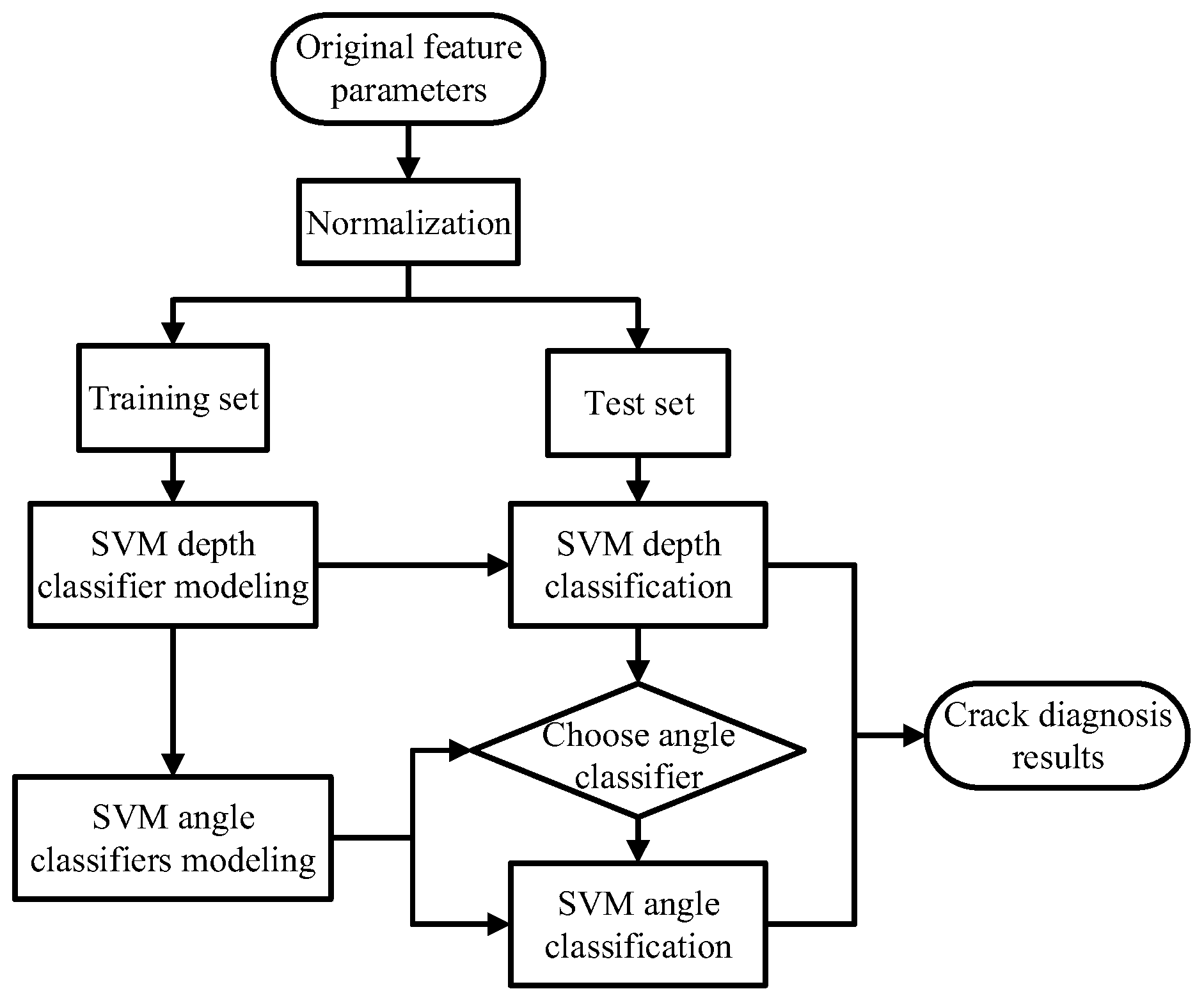
2. Support Vector Machine

The SVM uses the structural risk minimization principle, which minimizes the upper limit of generalization error and can solve problems such as small samples, overlearning, and local minima to construct the optimal hyperplane [21]. For other algorithms—taking the feed-forward neural network as an example—the sample data should be at least ten times larger than the number of model parameters, which can be calculated by (i × h + h × o) + (h + o), where i is the input number, h is the hidden layer size, and o is the output number. If the amount of data is too small, the generalization ability of the model algorithm is poor, and overfitting will occur. For the main project of quantitative detection of surface crack size using laser ultrasounds in this paper, the SVM method is suitable for quick and intelligent detection of oblique cracks’ depths and angles.

For multidimensional feature parameters in the input data samples, the algorithm system flow chart of this paper based on SVM to extract the crack depth and angle information is shown in Figure 1.

According to Figure 1, the input original feature parameters are first normalized and subsequently divided into a training set and a test set. For the test set, the created SVM depth classifier is used first to classify the data in depth. Subsequently, the corresponding angle classifier for angle classification based on the depth classification results is selected, and the crack extraction results are derived.

3. Finite Element Method Simulation and Results

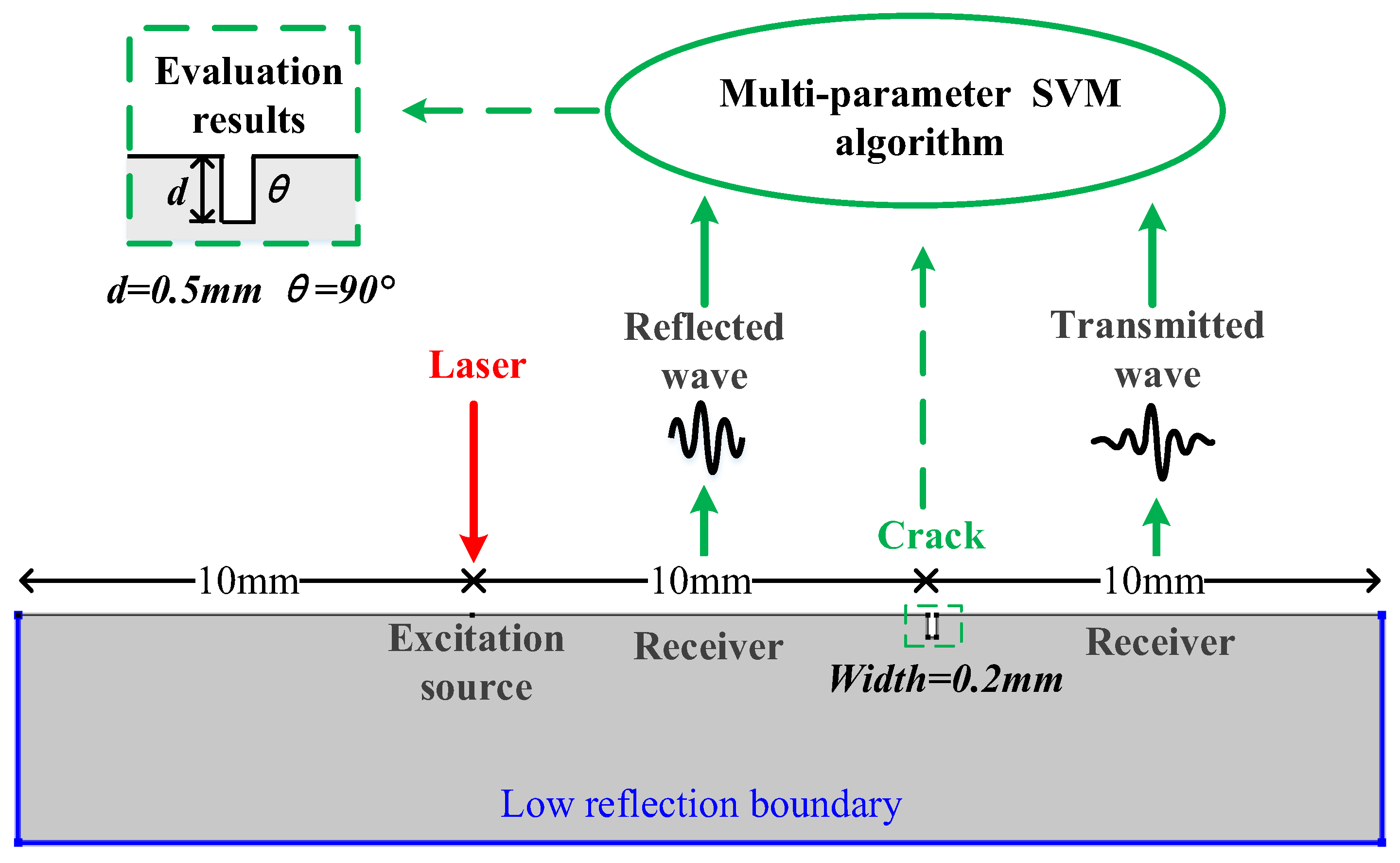
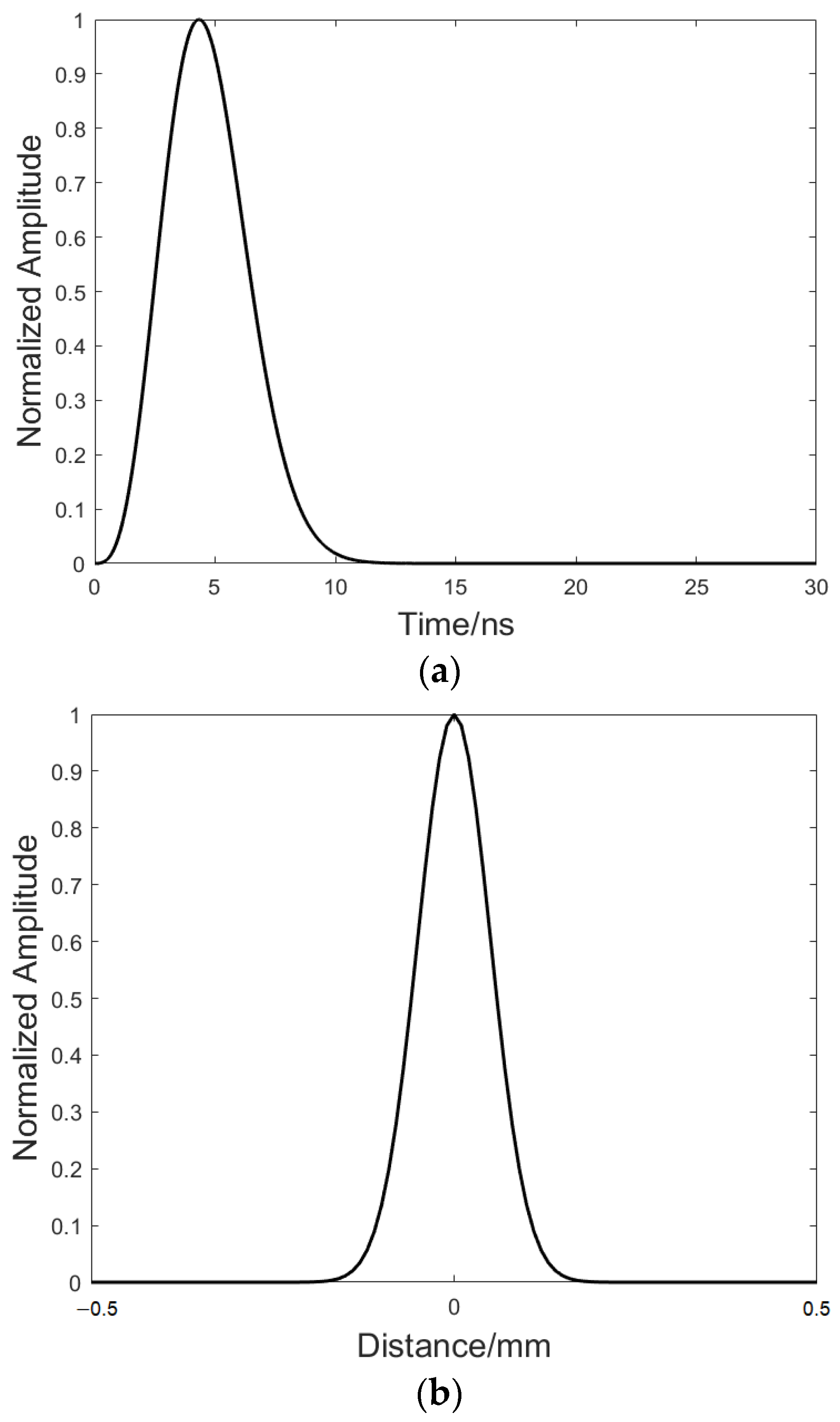
3.1. Simulation Setup

The COMSOL Multiphysics software, which is a useful tool to simulate coupled multiphysics using the FEM, is adopted in this paper to simulate laser ultrasounds. Two physical interfaces of thermal stress and solid mechanics and their coupling packages—thermal expansion and temperature coupling—are used to solve the simulation problem that contains the conversion of light energy, thermal energy, and acoustic energy during the laser ultrasound procedure generated in the finite solid medium. Laser-ultrasound-based mathematical models for thermal expansion and acoustic motion are shown in Equations (1) and (2):

$$k{\nabla }^{2}T=\rho c\dot{T}$$

(1)

$$\mu {\nabla }^{2}u+(\lambda +\mu )\nabla (\nabla \cdot u)=\rho \dot{u}+\beta \nabla T$$

(2)

where T is the temperature distribution at time t inside the sample; ρ, c, and k are the density, specific heat capacity, and thermal conductivity, respectively; u is the displacement field; β is the thermoelastic coupling coefficient; and λ and μ are Lamé constants. Equations (1) and (2) are coupled by the term $\beta \nabla T$. Finally, with the FEM, Equations (1) and (2) are solved using COMSOL software to obtain reflected and transmitted acoustic fields at oblique surface cracks. Due to the symmetric characteristic of the laser line source vertical to the scanning direction, a simplified 2D model is used by the FEM in this paper. Moreover, aluminum alloy, which is consistent with the following experimental arrangements, is chosen as the simulation material. The geometry of an FEM model, including laser source location, receiver location, crack depth and angle, as well as boundary condition is shown in Figure 2. The physical parameters of the simulated 2D model are presented in

Table 1. Physical parameters.

Thermal Conductivity (Wm−1K−1)	Thermal Expansivity (K−1)	Lamé Parameter λ (Pa)	Lamé Parameter μ (Pa)
238	2.3 × 10−5	5.1 × 1010	2.6 × 1010
Young modulus (MPa)	Poisson’s ratio (υ)	Density (kg/m3)	Thickness (d/mm)
7 × 104	0.33	2.7 × 103	5

.

With the COMSOL Multiphysics software, the grid type, grid size, simulation time step, and length are key parameters that seriously affect the simulation results. In the 2D FEM model, the laser line source is described by a product of two Gaussian functions in the spatial and time domains and shown as S(x,t) = g(t)*f(x). The expressions of g(t) and f(x) are:

$$g(t)=\frac{8t^3}{{\upsilon }^4}{e}^{-2t^2/{\upsilon }^2},f(x)=\frac{1}{\sqrt{2\pi }}\frac{2}{R_{\mathrm{G}}}{e}^{\raisebox{1ex}{$-2x^2$}\!\left/ \!\raisebox{-1ex}{$R_{\mathrm{G}}^2$}\right.}$$

(3)

where R_G is the Gaussian beam radius of 0.1 mm and υ is the laser pulse rise time of 5 ns. Two functions are shown in Figure 3. To satisfy the rule that the grid size is usually less than a quarter of the acoustic wavelength, a free triangle with a minimum element size of 0.01 mm, a maximum element size of 0.1 mm, a maximum element growth rate of 1.1, a curvature rate of 0.2, and a resolution of narrow regions of 10 are the element types in this built model. The simulation time length is 10 μs with a time step of 0.01 μs to satisfy the expression Δt = 1/(20f_max), where f_max is the central frequency of ultrasound. The 2D simulated model for laser ultrasounds takes 1 h and 16 min on a workstation with a 3.9 GHz CPU, 32 GB of memory, and a 512 GB hard disk.

The size of oblique cracks set on the surface of the specimen includes the depth and angle. Ten depths are used, nine of which are 0.2–1 mm per 0.1 mm, and the tenth depth is 1.2 mm. For each depth, 15 angles are considered; 5 angles are 22.5–52.5° at an interval of 7.5°, 6 angles are 60–120° at an interval of 10°, 3 angles are 120–135° at an interval of 7.5°, and the fifteenth angle is 150°. In total, 150 specimens are used to analyze the acoustic field at cracks to extract information on the crack size using the FEM method. Their data are used for SVM training in the following section.

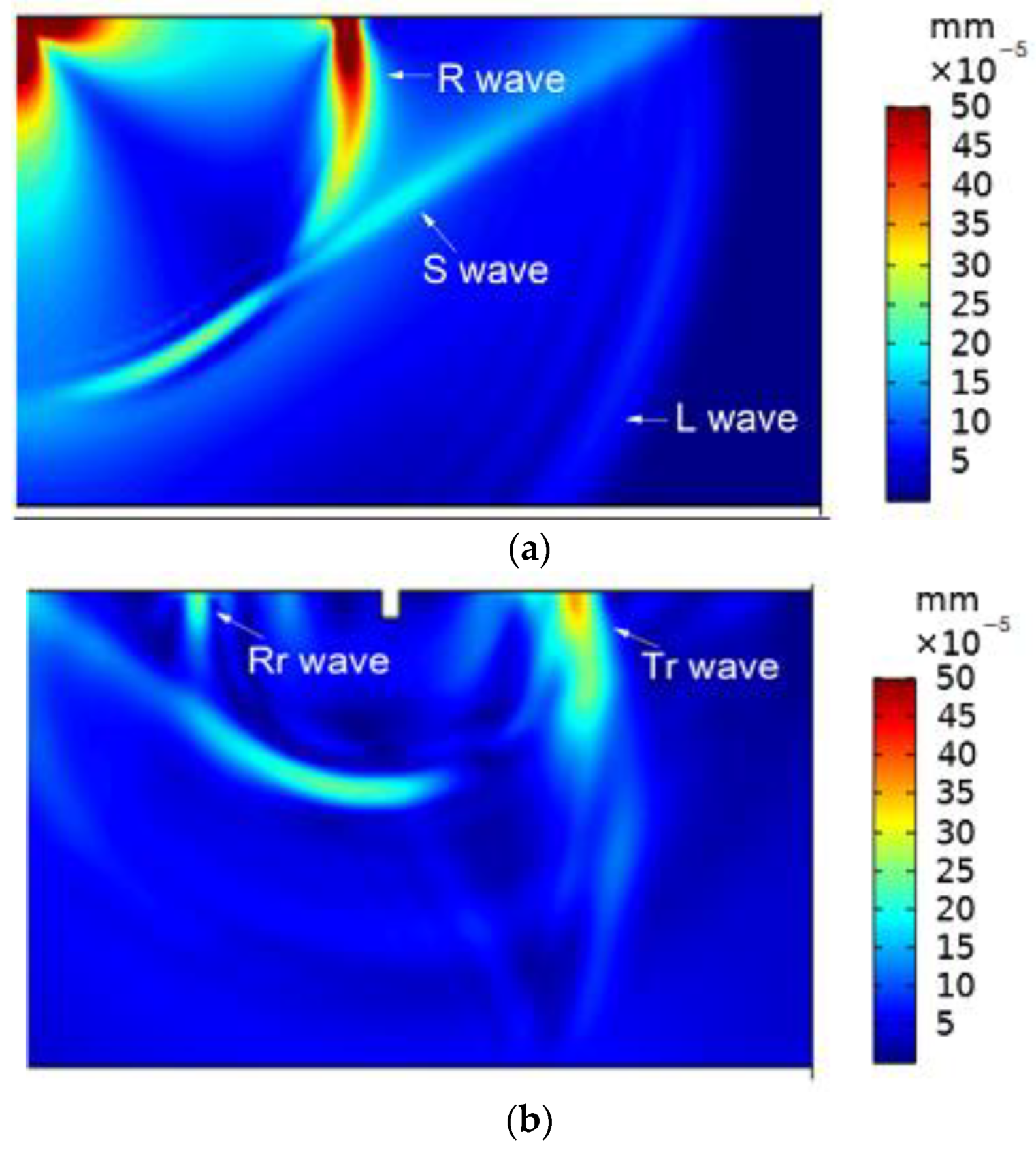
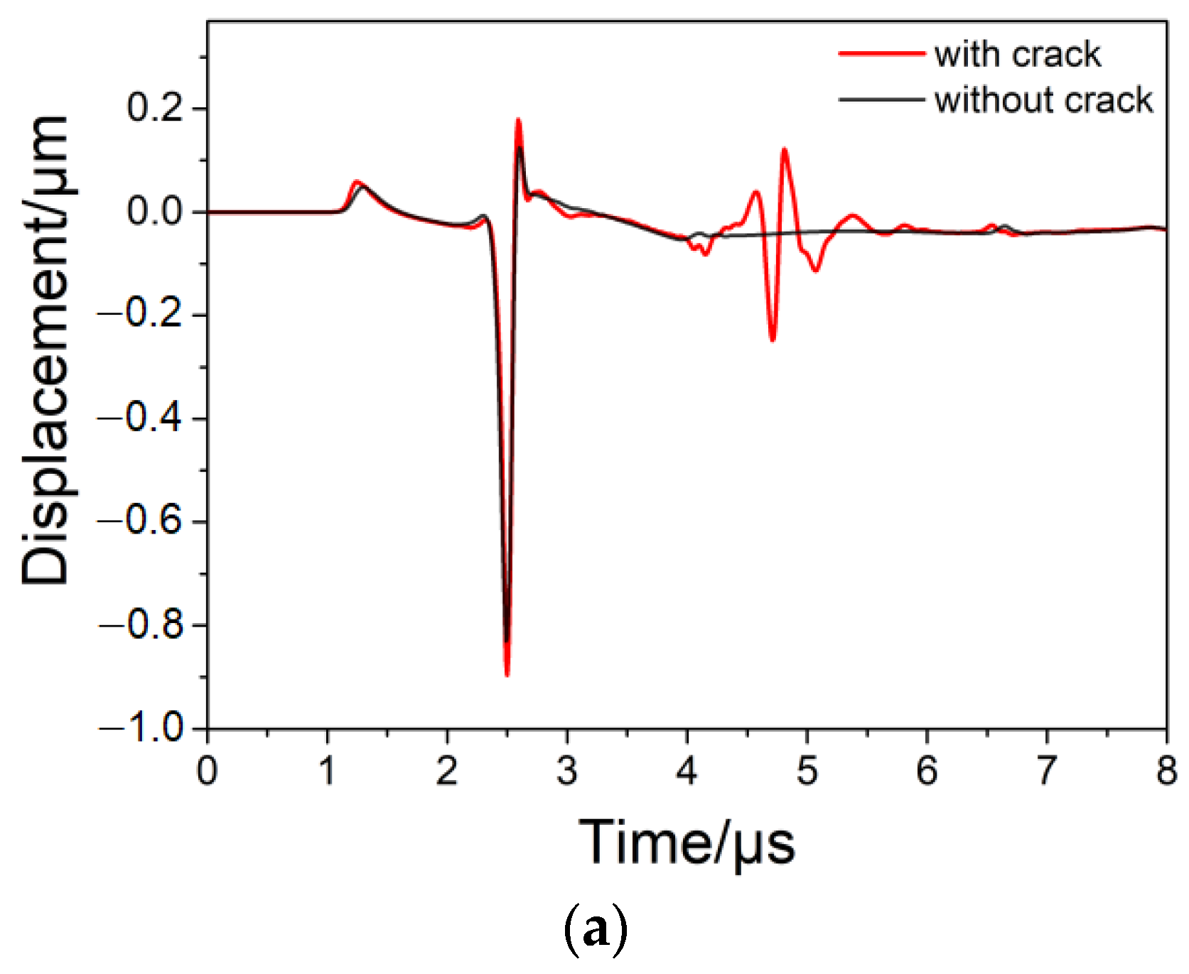
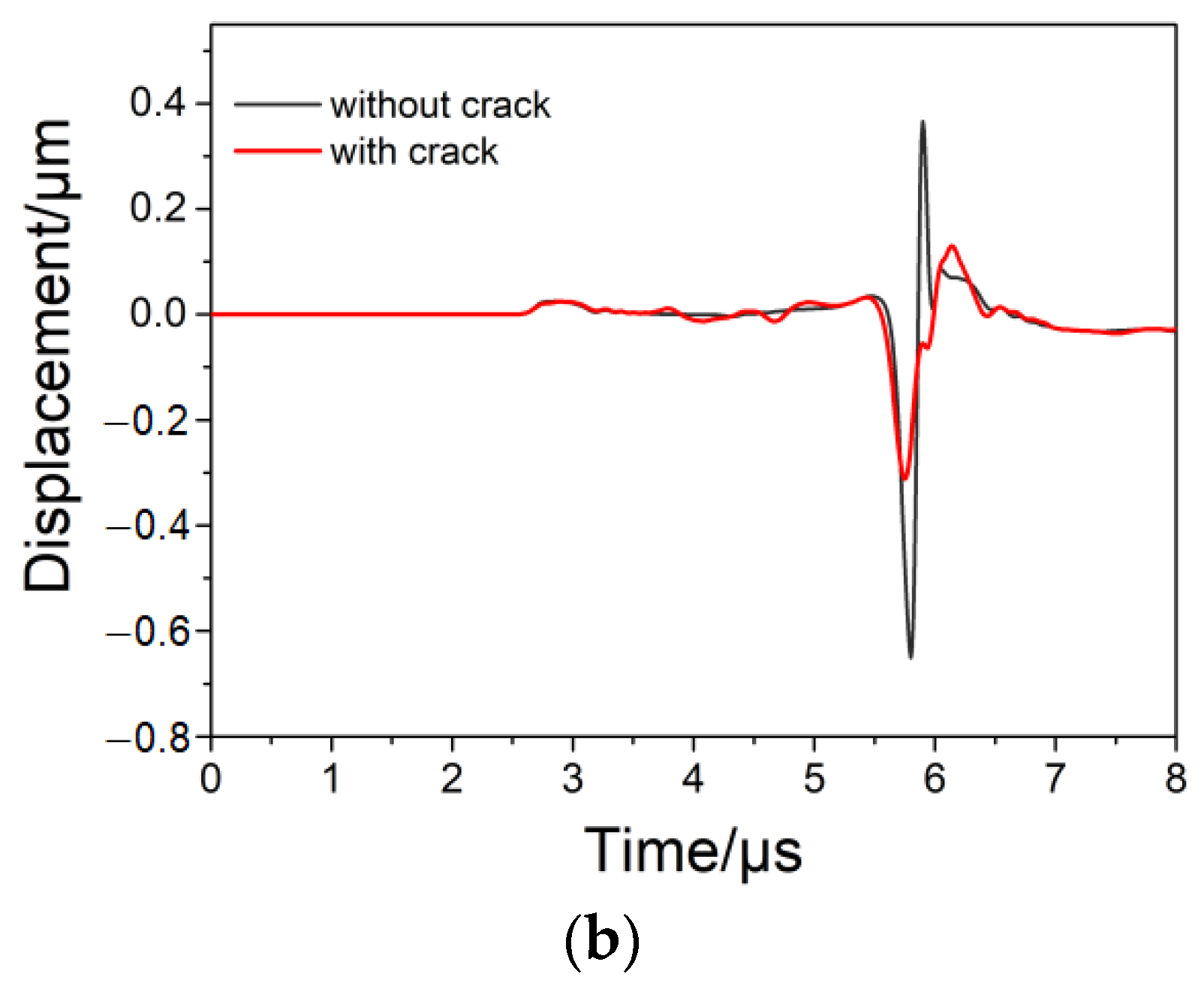
3.2. Simulation Results

Two displacement cloud images of the acoustic field generated by the laser at 1.33 μs and 3.34 μs are shown in Figure 4. The entire acoustic field at 1.33 μs generated by the laser, transverse wave (S wave), longitudinal wave (L wave), and surface Rayleigh wave (R wave) is shown in Figure 4a. Then, at 3.34 μs, the R wave continues to propagate along the surface of the material and encounters the oblique crack. Transmission and reflection acoustic fields at the crack are recorded in Figure 4b.

In Figure 4b, the surface wave interacts with the oblique crack. A part of the energy is reflected at the left edge of the oblique crack to form a reflected echo (Rr Wave), and the other part propagates along the oblique crack wall to the other side to form a transmission surface wave (TR Wave). The reflected wave and transmitted wave in the time domain are shown by the red line in Figure 5. Two reference signals are also acquired in the model without cracks and shown by the black line in Figure 5.

At 4.5 μs, a reflection wave is generated by the crack in (a), and the amplitude reduction of the transmitted wave is shown in (b). Therefore, the FEM method is helpful for simulating acoustic fields at cracks to acquire reflected and transmitted surface waves. The results in Figure 5 represent reflected and transmitted waves that carry crack information. However, the angles and depths of cracks cannot be directly detected in Figure 5.

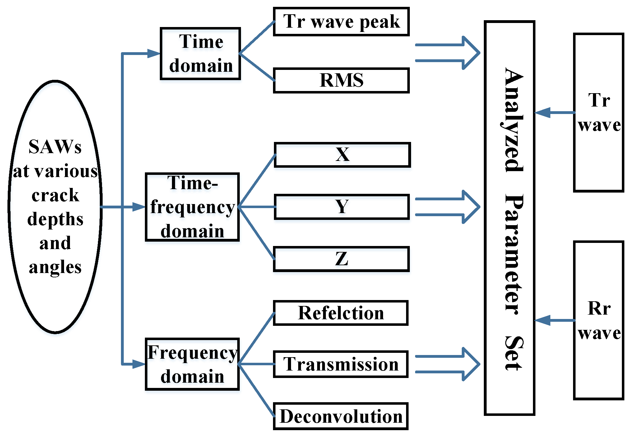
4. Feature Parameter Extraction

Feature parameters have a decisive impact on the accuracy of the SVM algorithm. To comprehensively describe the crack dimension, various parameters of reflected and transmitted waves in the time domain, frequency domain and time–frequency domain are extracted, as shown in Figure 6. In this section, the transmitted wave peak in Part A; root mean squares in Part B; transmission coefficient in Part C; reflection coefficient in Part D; deconvolution sum in Part E; and wavelet packet coefficient, wavelet packet energy peak, and wavelet packet entropy of both transmitted and reflected waves in Part F are analyzed. The feature parameters in Parts A and B are in the time domain; those in Parts C, D, and E are in the frequency domain; and those in Part F are in the time–frequency domain.

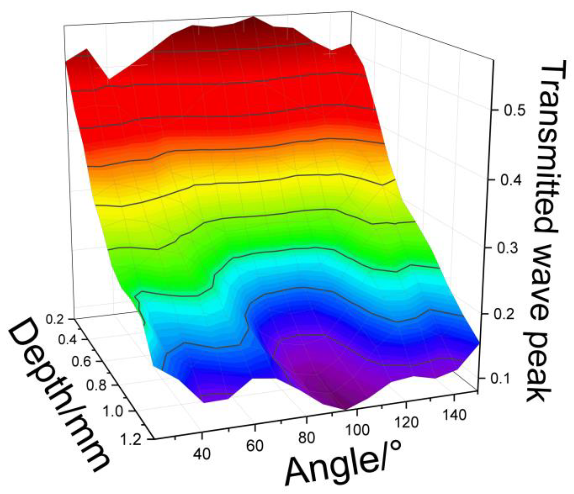
4.1. Transmitted Wave Peak

From the results of the FEM model presented in Section 3, the amplitude peaks of transmitted waves at cracks with depths of 0.2–1.2 mm and angles of 22.5–150° are extracted. Figure 7 shows 3D maps with angle on the X-axis, depth on the Y-axis, and normalized transmitted wave peak on the Z-axis. The color distribution in the legend reflects the normalized numerical values.

Figure 7 shows that the contour line bends upward by 90° where the peak values are lower, which reflects the symmetry of the transmission wave. The peak values gradually decrease with increasing depth. There is an obvious linear correlation between the peak values and the geometric information of cracks in Figure 7.

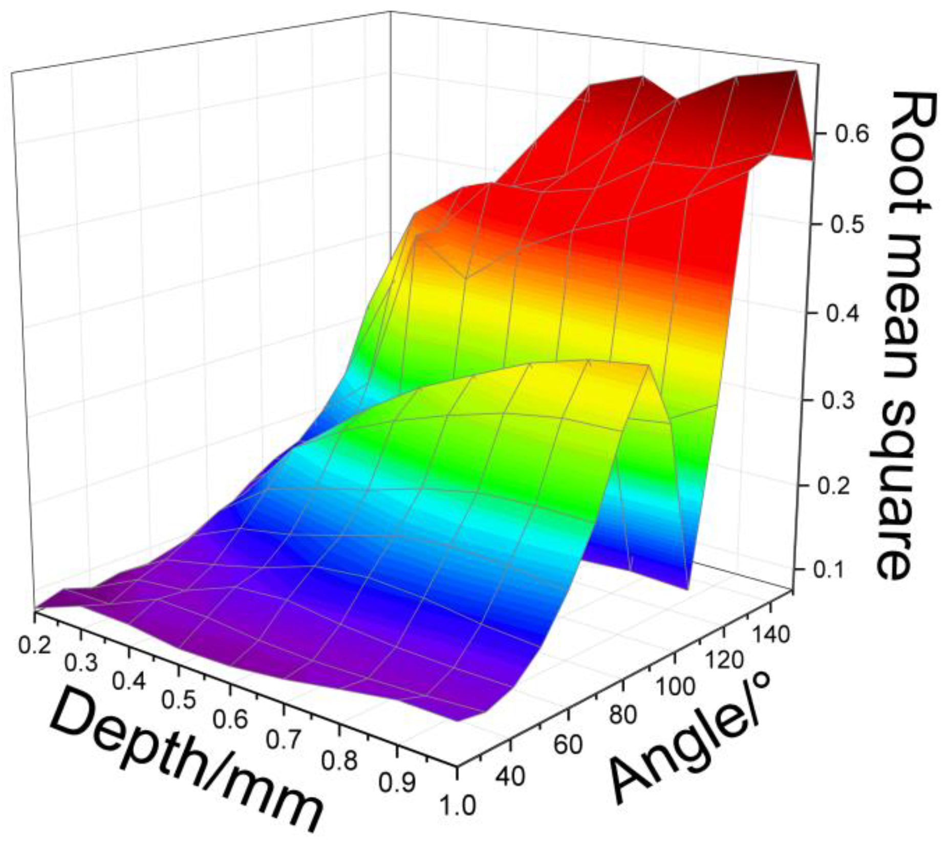
4.2. Root Mean Square

Similar to transmitted waves, reflected waves contain considerable crack geometry information. In the time domain, the root mean square of the reflected wave amplitudes is extracted and analyzed. Figure 8 shows a 3D map with angle as the X-axis, depth as the Y-axis, and normalized root mean square of the reflected waves as the Z-axis.

Figure 8 shows that the root mean squares have a rising, falling, and subsequently rising trend as the angles increase; however, they gradually increase when the depths increase. An obvious linear correlation between the root mean square of reflected waves and the geometric information of cracks is obtained. Therefore, the root mean squares of reflected waves are a good feature parameter for the SVM method.

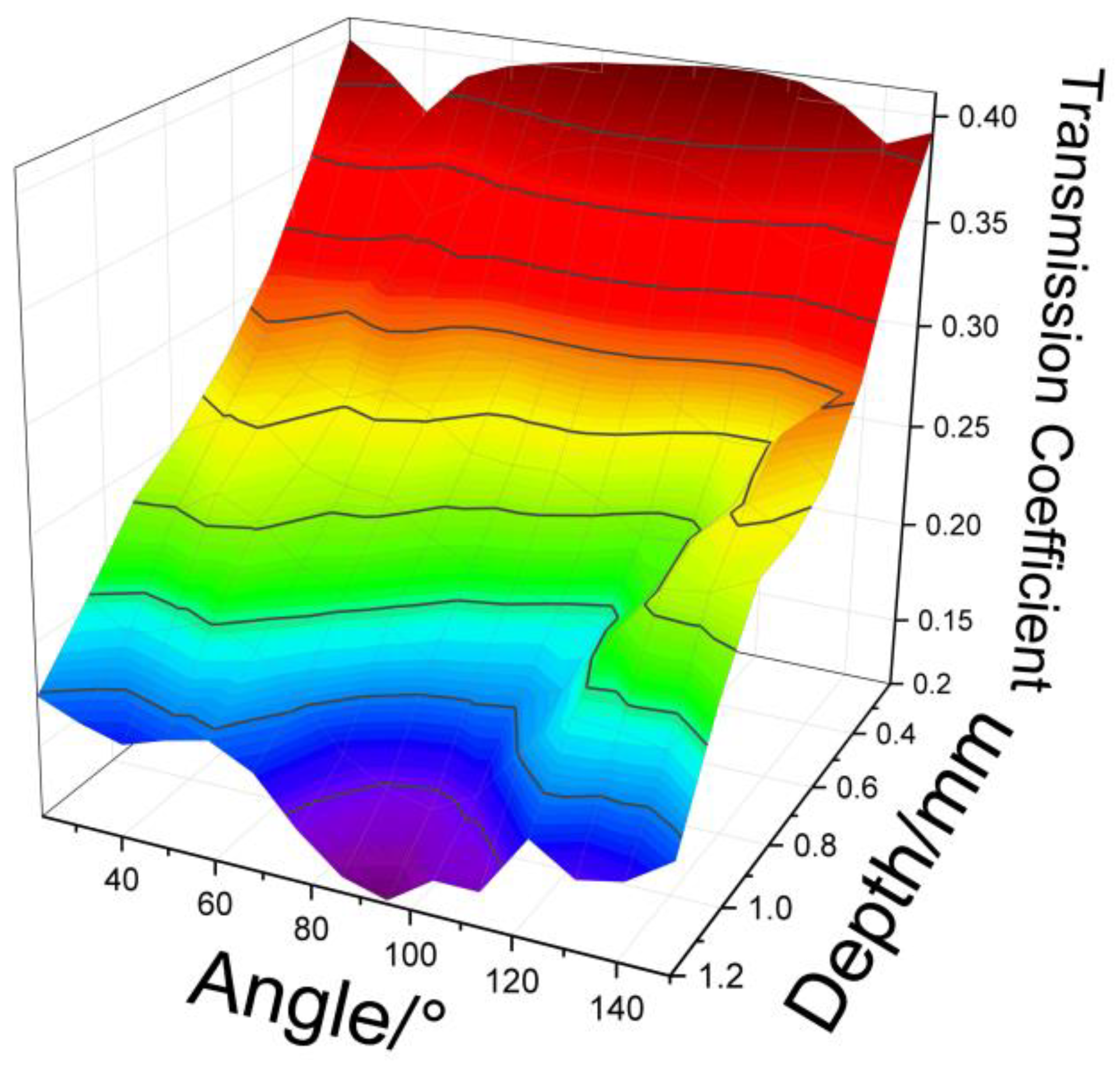
4.3. Transmission Coefficient

The transmission coefficient is defined as T = At/Ai, where At is the maximum value of the transmitted wave spectrum and Ai is the maximum amplitude of the direct wave spectrum. Figure 9 shows a 3D map with the depth as the X-axis, angle as the Y-axis, and transmission coefficient as the Z-axis.

Figure 9 clearly shows that the transmission coefficients gradually increase with decreasing depth. The contour line is curved upward at 90° and nearly parallel to the Y-axis when the depths are lower than 0.4 mm. Figure 8 also shows that angle has less influence on the transmission coefficient when the oblique crack depth is small.

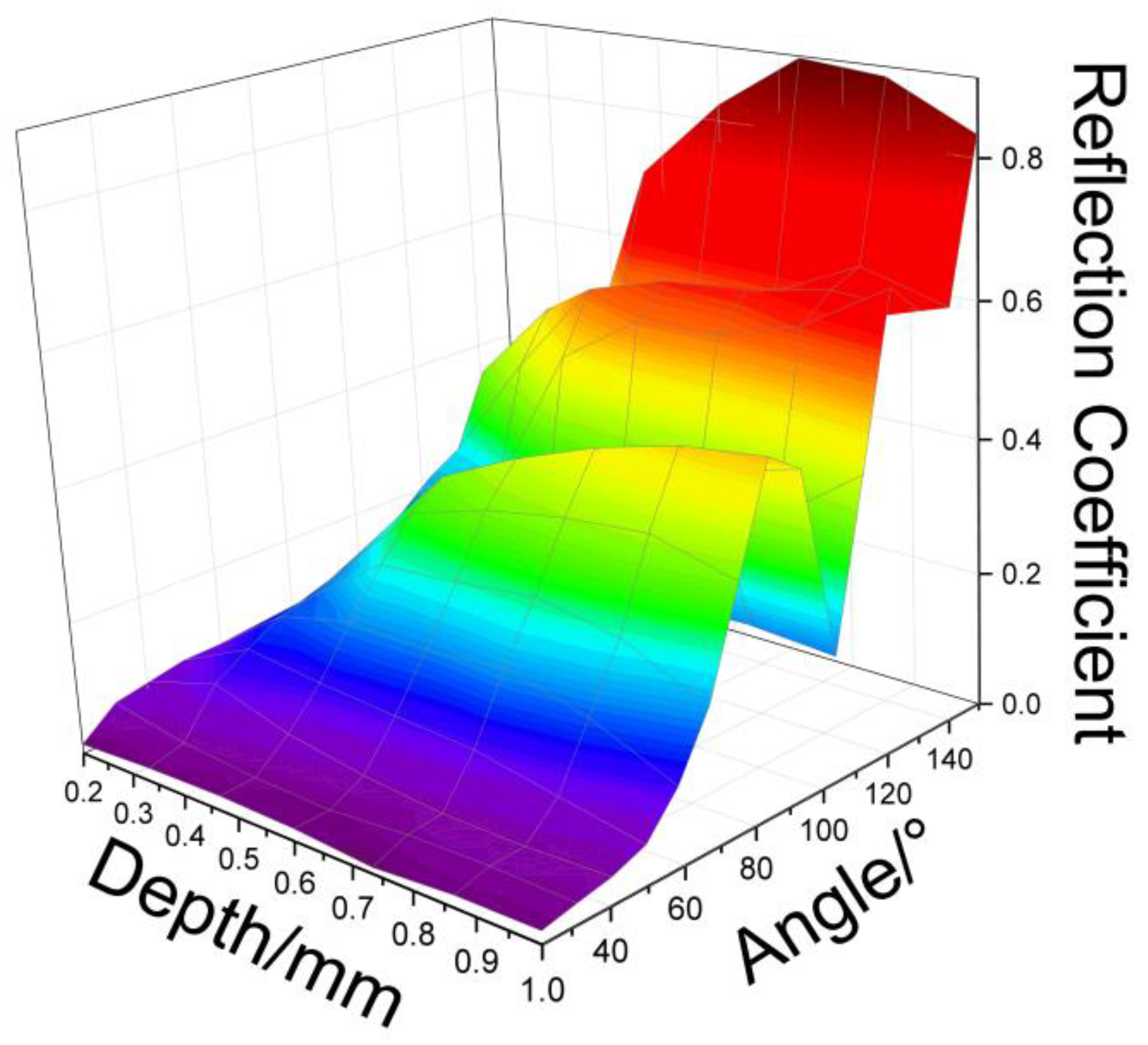
4.4. Reflection Coefficient

The reflection coefficient is defined as R = Ar/Ai, where Ar is the maximum value of the reflected wave spectrum, and Ai is the maximum amplitude of the direct wave spectrum to explore crack size information in the frequency domain. Figure 10 shows a 3D map with the angle as the X-axis, depth as the Y-axis, and reflection coefficient as the Z-axis.

Figure 10 shows that when the angle increases, the reflection coefficient values have a gradual upward trend, and the reflection coefficient values gradually increase when the depth increases. There is a linear correlation between the reflection coefficient and the geometric information of cracks. The reflection coefficient can be a class feature used by the SVM model to obtain class marks.

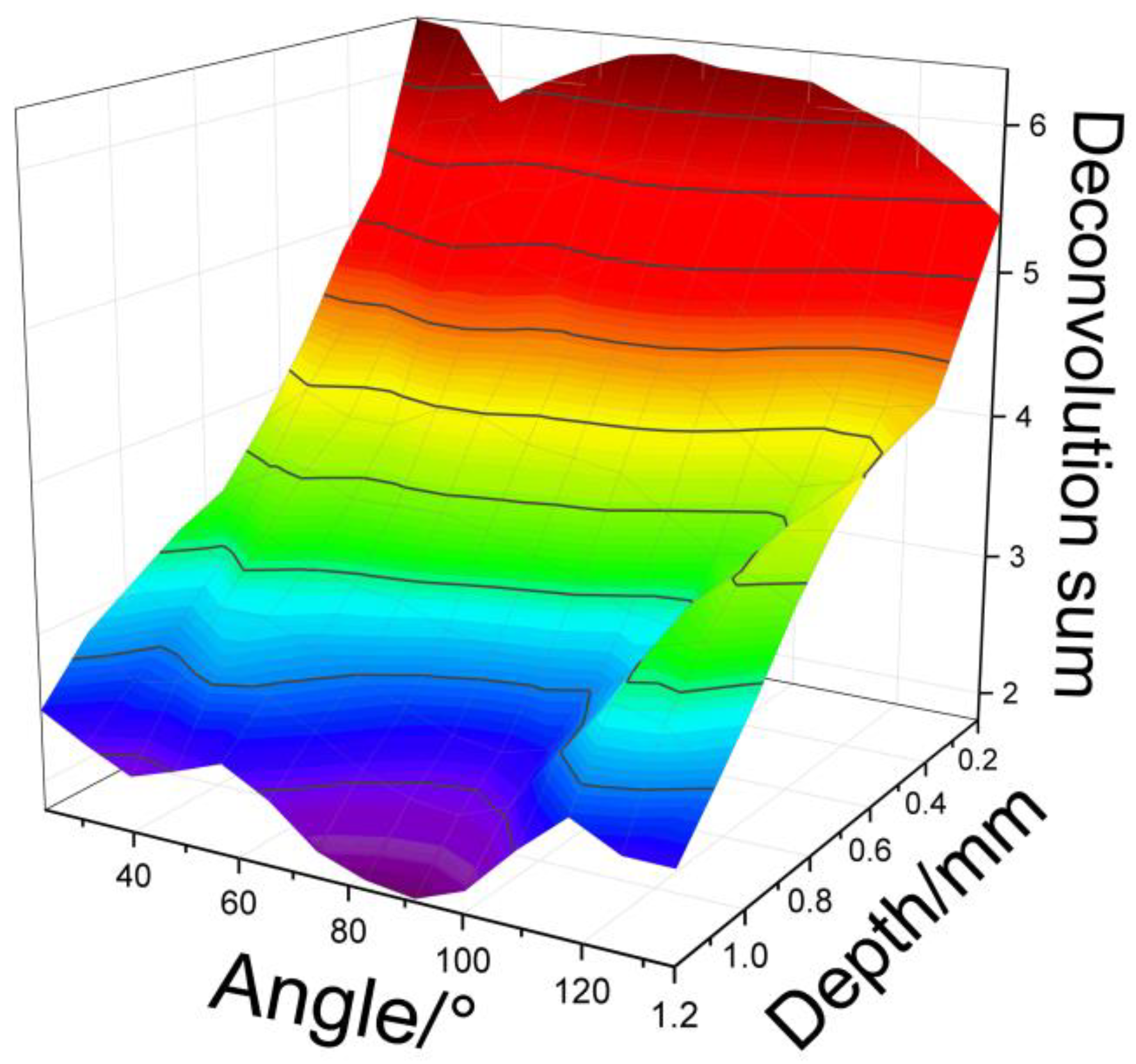
4.5. Deconvolution Sum

Oblique surface cracks are considered a system to process signals because they can reflect and transmit acoustic signals generated by lasers. Therefore, the transmitted wave signal y(t) as the output signal of the crack system is the convolution of the direct wave x(t) and the transfer function h(t) of the crack system, so they satisfy H(w) = Y(w)/X(w) in the frequency domain.

A deconvolution sum is obtained using the sum of values of H(w) in the frequency range related to the spectrum of the incident signal. The frequency range used by the deconvolution sum is 0.5–6.25 MHz in this paper. Figure 11 shows a 3D map with depth as the X-axis, angle as the Y-axis, and deconvolution sum as the Z-axis.

Figure 11 clearly shows that the deconvolution sum has a similar trend to the transmission coefficient in Part C. Therefore, both the deconvolution sum and the transmission coefficient can be feature parameters to obtain the crack depths and oblique angles using the SVM method.

4.6. Wavelet Packet Analysis

The wavelet packet (WP), which can divide the frequency band into multiple levels, is used to process acoustic signals containing considerable crack information. Wavelet packet analysis, which uses Sym8 as the wavelet basis to carry out five-layer wavelet packet decomposition, is performed on transmitted waves and reflected waves, and kernel principal component analysis (KPCA) is used to reduce the wavelet coefficient dimension according to [15].

In the time–frequency domain, WP coefficient peaks, WP energy peaks, and WP entropy are extracted and analyzed in this paper. Taking the transmitted wave as an example, the WP coefficient peaks, WP energy peaks, and WP entropy of transmitted waves at different crack depths and oblique angles are shown in Figure 12.

Figure 12 shows that when the depth increases, the WP coefficient peaks, WP energy peaks, and WP entropy shows different variation trends, which reflect different correlations with depth. Therefore, a selection standard is required to choose feature parameters that can fit the SVM model best and is proposed in the next section.

5. Feature Parameter Selection

Eleven feature parameters were extracted in Section 4. To improve the accuracy of the SVM algorithm and reduce the number of feature parameters, two standards to choose the feature parameters are analyzed in this section: the correlation coefficient between geometric information and a certain parameter and the correlation coefficient between feature parameters.

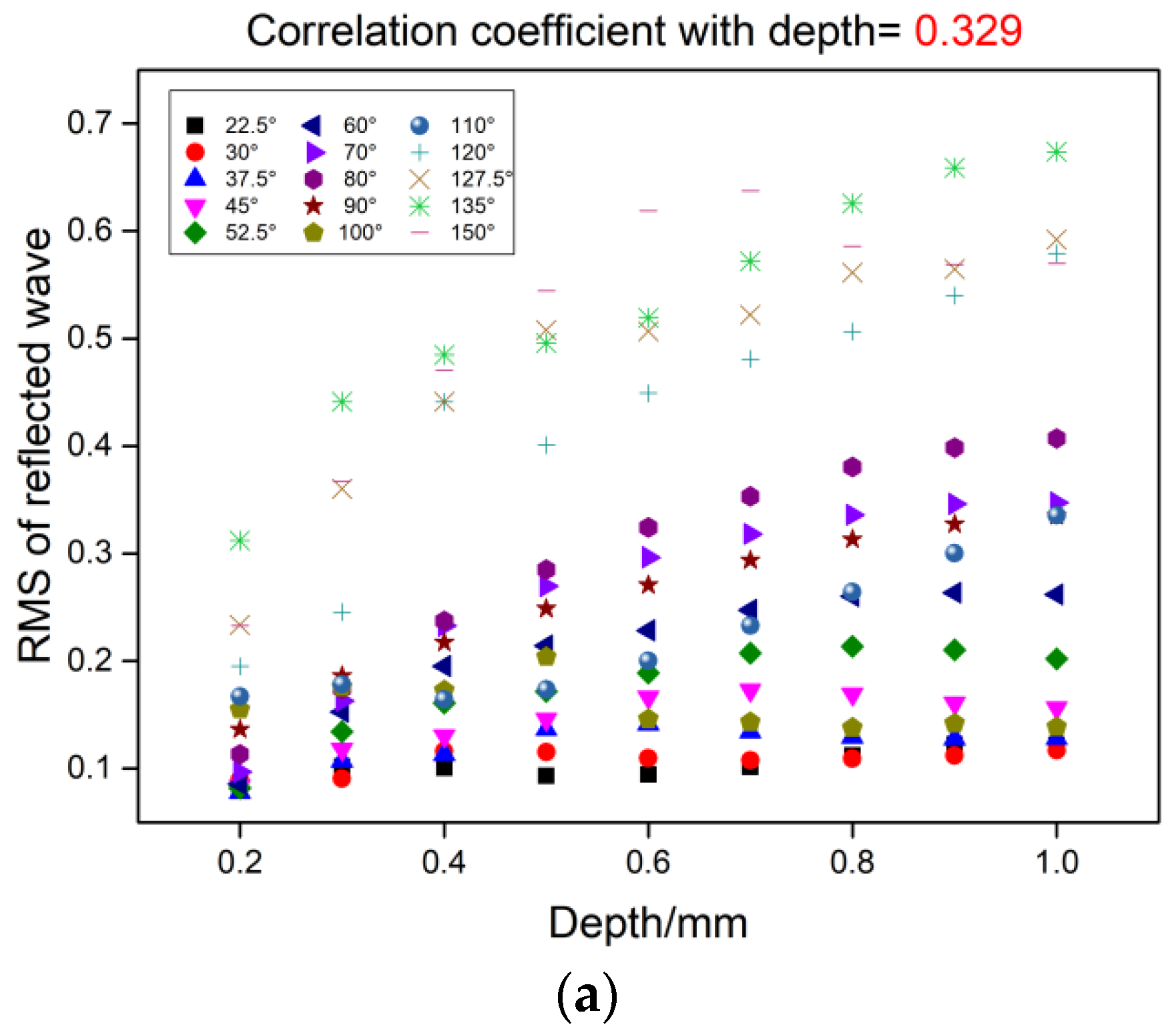
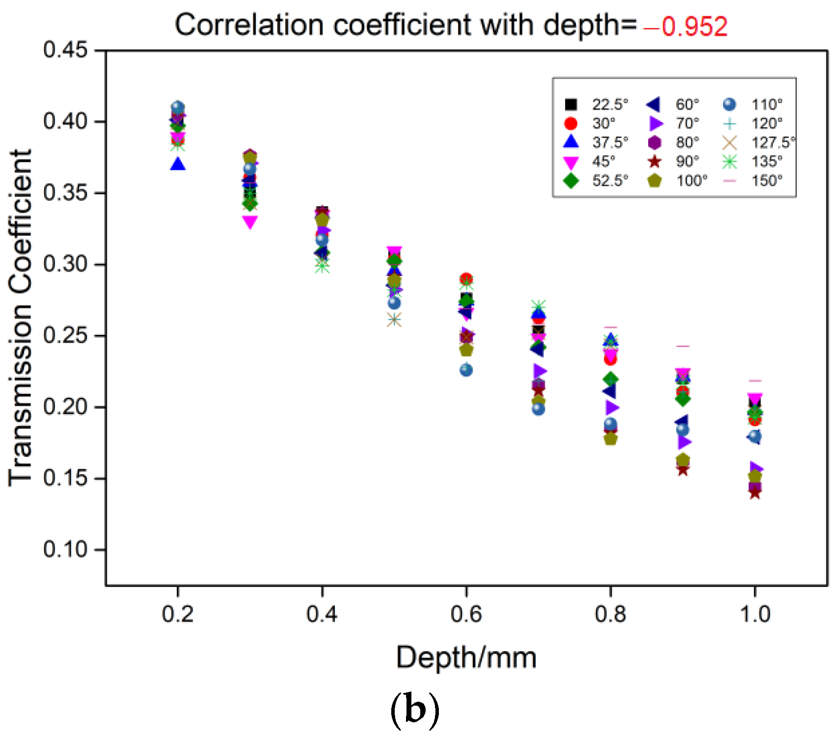
5.1. Correlation Coefficients between Geometric Information and Feature Parameters

Figure 13 shows a scatter plot of the root mean square of reflected waves in Part B and the transmission coefficients in Part C of Section 4. Their correlation coefficients versus depth are 0.329 and −0.952, respectively. When the correlation coefficient reaches 1, it is a completely positive correlation; when it reaches −1, it is a completely negative correlation.

Comparing Figure 13a,b, a greater linear relationship between transmission coefficient and depth is reflected by the larger correlation coefficient than that for the root mean square. Thus, the transmission coefficient is a better feature parameter to classify different depths. The prediction errors using the root mean square and transmission coefficient as feature parameters in the SVM model to realize depth classification are shown in Figure 14.

In Figure 14, the prediction errors of the transmission coefficient in (b) are lower than those of the root mean square in (a). The feature parameter with a higher correlation coefficient with the crack depth is included in the SVM model, and lower prediction errors are obtained. Therefore, the transmission coefficient has a better prediction ability to evaluate the crack depth by the SVM method. This result proves that the correlation coefficient between feature parameters and predicted geometric information is a selection standard to select suitable feature parameters for the SVM model. According to this selection standard, the correlation coefficients between the feature parameters and the crack depths and angles are shown in

Table 2. Selected correlation coefficients.

	Depth	Angle (0–90°)	Angle (90–180°)
Transmission coefficient	−0.952	−0.132	0.140
Transmitted wave peak	−0.911	−0.196	0.186
Deconvolution sum	−0.897	−0.062	0.230
Tr wave WP entropy	−0.829	−0.312	0.080
Reflection coefficient	0.238	0.852	0.667
Root mean square of reflected wave	0.329	0.766	0.712
Rr wave WP energy peak	0.116	−0.784	−0.443

and

Table 3. Other correlation coefficients for contrast.

	Depth	Angle (0–90°)	Angle (90–180°)
Tr wave WP coefficient peak	−0.105	0.316	−0.337
Tr wave WP energy peak	0.592	0.279	−0.066
Rr wave WP coefficient peak	0.066	−0.654	−0.137
Rr wave WP entropy	−0.104	0.734	0.487

, respectively. The higher correlation coefficients (absolute value > 0.6) in the tables are shown in red for clarity.

In total, seven feature parameters are chosen in this paper, as shown in Table 2. In Table 2, the transmission coefficient, transmitted wave peak, deconvolution sum, and Tr wave WP entropy have absolute correlation coefficients greater than 0.8 with the crack depth, which shows an excellent ability to evaluate the crack depth according to the correlation coefficient standard. The reflection coefficient, the root mean square of the reflected wave, and Rr wave WP energy peak have a good correlation with the angle. They are chosen as feature parameters for crack angle evaluation. The Rr wave WP energy peak has a correlation coefficient of −0.433, which is less than 0.6 at angles of 90–180°. The angle evaluation in this paper involves two parts: 0–90° and 90–180°. Although the Rr wave WP energy peak has a low correlation with angles of 90–180°, it can still be a feature parameter for the angle evaluation because it has a good correlation with angles of 0–90°. In Table 3, the Tr wave WP coefficient peak and Tr wave WP energy peak have absolute correlation coefficients below 0.6. According to the correlation coefficient standard, these feature parameters are not chosen for the SVM model for crack depth and angle evaluation. Notably, the Rr wave WP coefficient peak and Rr wave WP entropy have a correlation value above 0.6 at angles of 0–90°. However, they are not selected as feature parameters because these two parameters have low correlation with angles of 90–180°, and the correlation with angles of 0–90° is not sufficiently high. Another important reason is expounded in the following section: the correlation coefficients among the feature parameters as another selection standard must be considered and discussed. Overall, transmitted waves are mainly related to crack depths, and reflected waves are mainly related to crack angles. The correlation coefficient standard is necessary to choose feature parameters for the SVM model to improve the prediction accuracy for crack depths and angles.

5.2. Correlation Coefficients among Feature Parameters

The SVM algorithm in this article is a multiparameter algorithm, so the correlations with crack geometry information and the correlations among the parameters should be considered. The correlation coefficients among the selected feature parameters are shown in

Table 4. Correlation coefficients among the selected parameters.

	A	B	C	D	E	F	G
A	1
B	0.979	1
C	0.951	0.929	1
D	0.811	0.848	0.679	1
E	−0.285	−0.301	−0.162	−0.347	1
F	−0.338	−0.335	−0.256	−0.362	0.943	1
G	0.004	0.044	−0.091	0.071	−0.734	−0.597	1

Note: A: Transmission coefficient, B: transmitted wave peak, C: deconvolution sum, D: Tr wave WP entropy, E: reflection coefficient, F: root mean square of reflected wave, G: Rr wave WP energy peak.

.

In Table 4, the smallest value of 0.004 is the correlation between the transmission coefficient and the Rr wave WP energy peak. The transmission coefficient is a feature parameter of transmission waves in the frequency domain; however, the Rr wave WP energy peak is a feature parameter of reflected waves in the time–frequency domain. Because the frequency domain and time–frequency domain are two different domains and the transmitted waves and reflected waves are uncorrelated, the transmission coefficient and Rr wave WP energy peak have the lowest correlation value. Therefore, the correlation coefficients in different domains or determined by different wave generation methods are small. This result also suggests that a comprehensive analysis is required in the parameter extraction process to obtain higher accuracy.

There is another reason for not choosing the Rr wave WP coefficient peak and Rr wave WP entropy as feature parameters. As discussed in Part A, the Rr wave WP coefficient peak and Rr wave WP entropy are not included in the SVM model partly due to their low correlation with angles of 90–180°. However, another reason is that these two feature parameters have a high correlation with the Rr wave WP energy peak, which has been selected as a feature parameter for the SVM model. The correlation coefficients of the Rr wave, WP coefficient peak, and Rr wave WP entropy with the Rr wave WP energy peak are shown in

Table 5. Coefficients between the selected parameter and others.

	Rr Wave WP Energy Peak.
Rr wave WP coefficient peak	0.770
Rr wave WP entropy	−0.976

.

In Table 5, the correlation coefficient between the Rr wave WP coefficient peak and the Rr wave WP energy peak is 0.770, and the correlation coefficient between the Rr wave WP entropy and the Rr wave WP energy peak is −0.976. Compared to Table 4, the values of these two correlation coefficients are sufficiently high to exclude the Rr wave WP coefficient peak and Rr wave WP entropy as feature parameters.

To further expound the necessity of the selection standard using correlation coefficients among the feature parameters, we assume that the transmission coefficient is selected as a feature parameter in the SVM model to evaluate the crack depth. The deconvolution sum and Tr wave WP entropy are analyzed as other potential feature parameters for the SVM model. The correlation coefficient between transmission coefficient and deconvolution sum is 0.951, and the correlation coefficient between the transmission coefficient and Tr wave WP entropy is 0.811. The differences between their SVM prediction errors are shown in Figure 15.

In Figure 15, the SVM model, which uses the transmission coefficient and deconvolution sum as the feature parameters, is defined as A. The SVM model, which uses the transmission coefficient and Tr wave WP entropy as the feature parameters, is defined as B. The results show that B has lower prediction errors than A. It is known that the correlation coefficient of the two feature parameters in B is smaller than that of A (0.811 < 0.951). Thus, the correlation between feature parameters significantly affects the prediction accuracy of the SVM algorithm. Therefore, the feature parameters should be chosen for the SVM model by comprehensively considering the selection standard in Part A and Part B. The detailed rule is that when the correlation coefficients between feature parameters and crack geometry information are larger and the correlation coefficients between feature parameters themselves are smaller, a higher prediction accuracy is achieved. The reason is that the feature parameter, which has a larger coefficient with crack geometry information according to the selection standard in Part A, can provide a more accurate prediction. Higher correlation coefficients among feature parameters imply that these feature parameters contain similar prediction information.

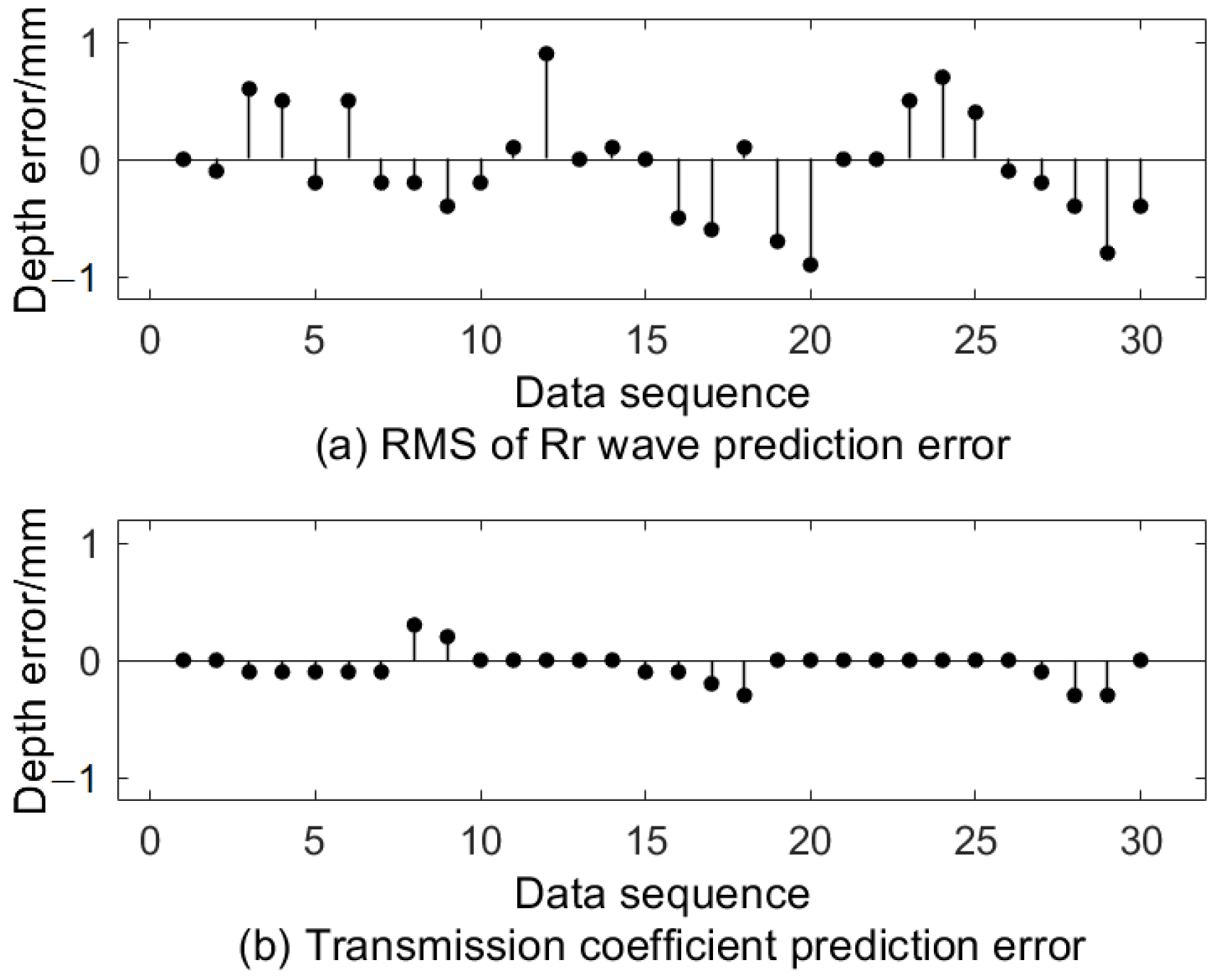
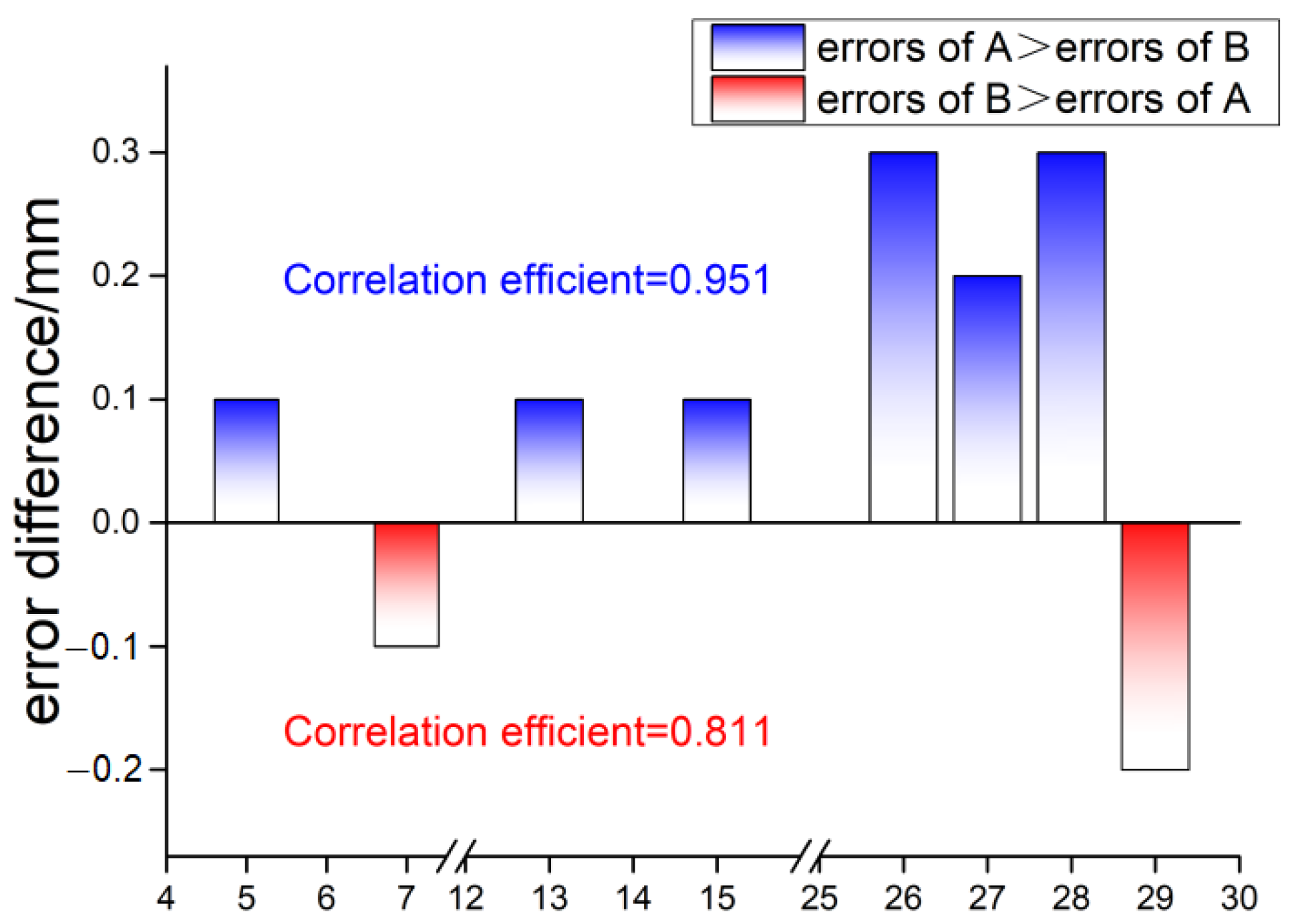
6. Simulation Evaluation Results

The data set includes 180 data samples covering 10 crack depths and 15 angles and is divided into 150 training samples and 30 test samples. The input parameter number of the SVM model is 7, and the output parameter number of the SVM model is 10 depths and 15 angles in this paper, so there must be at least 1720 samples for training if a feed-forward neural network with nine hidden layers is used. Therefore, the number of samples in this work for training satisfies the quantity for small samples.

To show the linear relationship between feature parameters and crack depths and angles, seven feature parameters selected in this paper of 150 training samples are converted to one-dimensional data of 150 training samples adopting the KPCA method.

KPCA is a widely used method in data dimension reduction. This method can minimize the loss of information while compressing the data and retain the overall characteristics of all feature parameters. In this paper, the KPCA method is adopted to convert seven feature parameters to one KPCA parameter, which can show the overall relationship between the selected parameters and the crack geometry information.

Figure 16 shows the 3D map with depth as the X axis, angle as the Y axis, and the normalized feature parameter as the Z axis.

In Figure 16, when the depths and angles increase, the feature parameter gradually decreases. There is a good correlation between the feature parameter and the crack depths and angles. Therefore, the feature parameters are suitable for the SVM model to predict the crack depths and angles.

Using the feature parameters, the depth and angle prediction results and the actual depth and angle sequences are shown in Figure 17.

Figure 17 shows that the correct rate of crack depth prediction in the depth range of 0.2–0.6 mm reached 100%. All error values are only one depth step. Figure 17c,d show that the accuracy of angle prediction reached 100% in the angle range of 22.5–70°, 90–120°, and 135–150°. The prediction results of depth and angle error sequence diagrams using different numbers of parameters are shown in Figure 18 and Figure 19.

In Figure 18 and Figure 19, the five parameters in (a) are the seven selected parameters except for the Tr wave WP entropy and Rr wave WP energy peak. The nine parameters in (c) are the seven selected parameters, Tr wave WP coefficient peak, and Rr wave WP coefficient peak. The depth and angle classification errors of this paper using the seven-parameter SVM model are shown in Figure 18b and Figure 19b, respectively.

In Figure 18a–c and Figure 19a–c, the depth and angle prediction errors using five, seven and nine feature parameters are shown, respectively. In Figure 18a–c, the error numbers are eight, four, and six, respectively. Figure 19a–c also show that the prediction angle errors using the seven parameters in (b) are the smallest. The results show that the seven chosen parameters have the best ability for evaluating oblique crack depths and angles, which also verifies the correctness of the proposed feature parameter selection standards. Therefore, this article selects these seven feature parameters to predict crack depth and angle.

7. Experimental Verification

7.1. Experimental Setup

A schematic block diagram of the laser ultrasonic testing experimental platform in the work is shown in Figure 20. In the hardware system of the laser ultrasound platform, a CFR200 laser transmitter was adopted to excite a laser with a wavelength of 1064 nm, a repetition frequency of 20 Hz, and a pulse width of 11 ns. Then, the emitted laser was focused into a line source on the surface of the specimen by a lens with a focal length of 100 mm. Surface waves generated by the laser line source propagated in two opposite directions along the surface of the detected specimen. The QUARTET-500 mV receiver equipment based on the Michelson interference principle was adopted as the receiver of the laser ultrasound platform. Finally, due to the laser emitter and receiver parts, a total noncontact laser ultrasound platform was built. The sampling frequency, scanning distance, step, and direction were set through LU Scan software. The time length was 20 μs with a time step of 0.02 μs. The scanning step and distance were 0.05 mm and 30 mm, respectively. The acquired signals were saved and processed to put into the multiparameter SVM model.

The 110 groups of experimental data containing eleven angles (30°, 45°, 60°, 70°, 80°, 90°, 100°, 110°, 120°, 135°, 150°) were randomly selected; 88 groups were selected as the training set, and the remaining 22 groups were selected as the test set. Sixty groups of experimental data of six depths (0.1–0.6 mm) were randomly chosen; 48 groups were selected as the training set, and the remaining 12 groups were selected as the test set. The experimental data were a set of small samples applicable for the quantity of the SVM method.

7.2. Experimental Result Discussion

Based on the above experimental platform, the 3D and 2D plots of the B-Scan images of oblique cracks with angles of 60°, depths of 0.5 mm, and widths of 0.2 mm are shown in Figure 21.

In Figure 21, the direct wave, transmitted wave, and reflected wave are labeled. There is a significant reduction in amplitude when a direct wave interacts with an oblique crack. Part of the direct wave reflected by the crack forms the Rr wave, and when the crack approaches the laser source, the Rr wave is gradually generated near the direct wave. The other part of the direct wave that propagates along the oblique crack wall forms a Tr wave. The initial and denoising signals of the transmitted wave and direct wave are extracted from the corresponding areas of the B-Scan image. The Rr waves are extracted from data from scanning distances of 2.5–3 mm. The Tr waves are extracted from data from scanning distances of 10–10.5 mm. The Tr wave and Rr wave are shown in Figure 22 and Figure 23.

Figure 22 and Figure 23 clearly show the positions of the transmitted wave, direct wave and reflected wave. The seven feature parameters based on experimental signals are included in the SVM model. Then, to show the linear relationship between the crack angle, depth, and experimental data, the data of seven feature parameters are transferred to one dimension using the KPCA method. The results are shown in Figure 24 and Figure 25.

In Figure 24 and Figure 25, the normalized feature parameters of the experimental data are denoted by dots, and the fitting lines are denoted in red. The determination coefficients of the fitting curves in Figure 24 and Figure 25 are 0.842 and 0.771, respectively. The fitting curve of the angles has a better linear relation than that of the depths. Moreover, the distance from the data of crack depth at 0.3 mm to the fitting curve is 0.11772, which is larger than the other two data of the crack depth at 0.4 mm and 0.5 mm at the distances of 0.05528 and 0.09352, respectively, as shown in Figure 25. Then, the evaluated crack angles and depths of the tested specimens are shown in Figure 26b and Figure 27b and compared to the actual sequence in Figure 26a and Figure 27a.

Figure 26a shows the actual angles versus 22 data points using stems. Both 1–11 data points and 12–22 data points are two test sets denoting 11 angles at 30°, 45°, 60°, 70°, 80°, 90°, 100°, 110°, 120°, 135°, and 150°. After the angle prediction using the SVM model, Figure 26b shows the evaluated results for two test sets at angles of 30°, 45°, 60°, 70°, 80°, 90°, 100°, 110°, 120°, 135°, and 150°. By successively comparing the value at each data point in Figure 26a,b, we obtain the errors between actual angles and evaluated angles as presented in Figure 28a. The prediction errors only occur at an angle of 110° at the 19th data point, which belongs to the second test set. The SVM model using seven feature parameters in this work trains 88 samples into 11 angles. Its accurate classification rate is 95.5% for experimental data. Highly accurate angle measurements using the SVM based on laser ultrasonics are obtained for inclined surface cracks.

In Figure 27, 12 data points are shown using stems for the actual depth (a) and evaluated depth (b). Here, data points 1–6 and data points 7–12 are one test set, which is described at 0.1 mm, 0.2 mm, 0.3 mm, 0.4 mm, 0.5 mm and 0.6 mm. Similar to the angle prediction process, two test sets are used for the depth measurement. The prediction errors between the actual depths in 27(a) and the evaluated depths in 27(b) are shown in Figure 28(b), where the measurement errors occur at the third data point and ninth data point, which are the depths of 0.3 mm. The evaluated error is 0.1 mm. The SVM model set using seven feature parameters in this work trains 48 samples that are classified into six depths. The accurate classification rate is 83.3%, which is lower than the accuracy rate of the angle classification. The coefficient of the fitting curve in Figure 25 is smaller than that in Figure 24, which illustrates that the relationship between the normalized feature parameter and the angles is less linear. In Figure 25, the data are farthest from the fitting curve at a crack depth of 0.3 mm, which causes the failure of its depth evaluation. The depth measurement using SVM based on laser ultrasonics is well accomplished in this work.

The prediction errors can be reduced by increasing the number of angle and depth classes. The simulated and experimental results show the applicability of the SVM algorithm in the classification of small sample data and prove the feasibility of the SVM algorithm for the quantitative measurement of surface cracks using laser ultrasonics in this paper in practical applications.

8. Conclusions

In this paper, seven feature parameters in the time domain, frequency domain, and time–frequency domain are analyzed and selected according to two proposed feature parameter selection standards and put into the SVM model to measure the angle and depth of oblique surface cracks. To explore the feature parameter selection standards, the correlation coefficients between crack geometry information and feature parameters and between the selected feature parameters themselves are analyzed. To verify this SVM model, a 2D FEM model is built to acquire ultrasound signals to extract seven feature parameters and subsequently include them in an SVM model. Finally, comprehensive verification by FEM simulation and experimental data is conducted.

The conclusions are as follows:

(1)

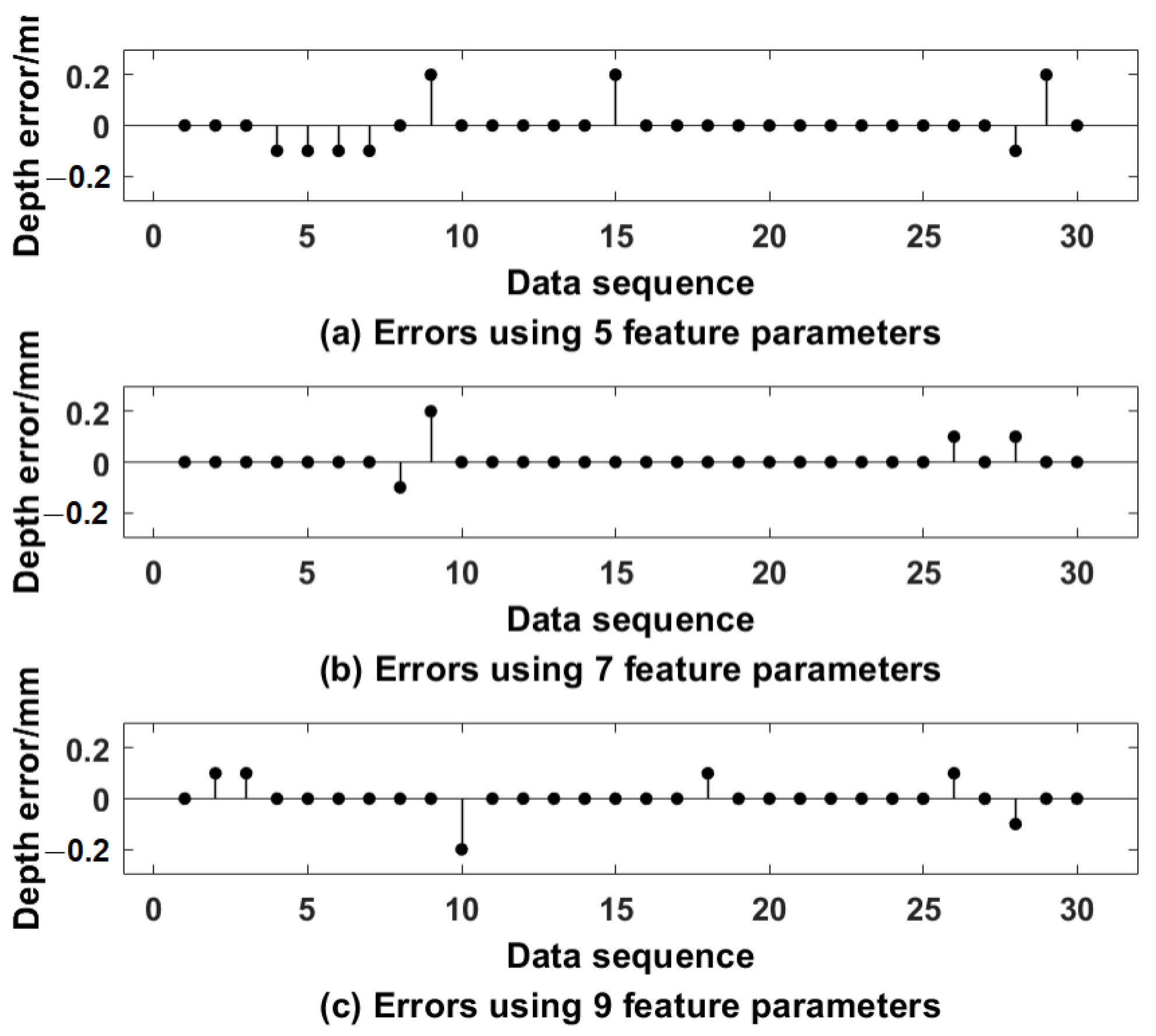
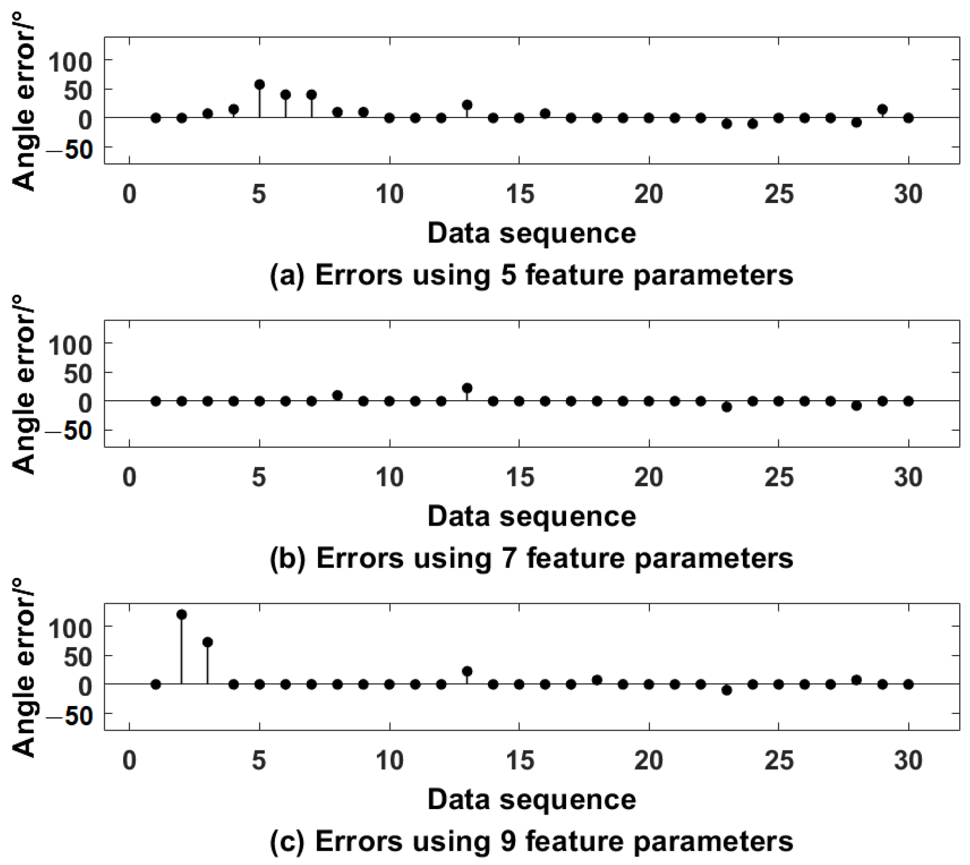
The five-parameter SVM model, seven-parameter SVM model, and nine-parameter SVM model are compared using the FEM. The best prediction results are obtained using a seven-parameter SVM model. The results also show that the selected feature parameters in this paper are suitable for the SVM model to nondestructively detect surface crack depths and angles.

(2)

This paper shows that the SVM method is suitable for laser ultrasound to quantitatively detect oblique surface cracks, and its advantages are especially revealed when the amount of training set is small sample data. All of the training sets used in this paper satisfy the definition of a small sample.

(3)

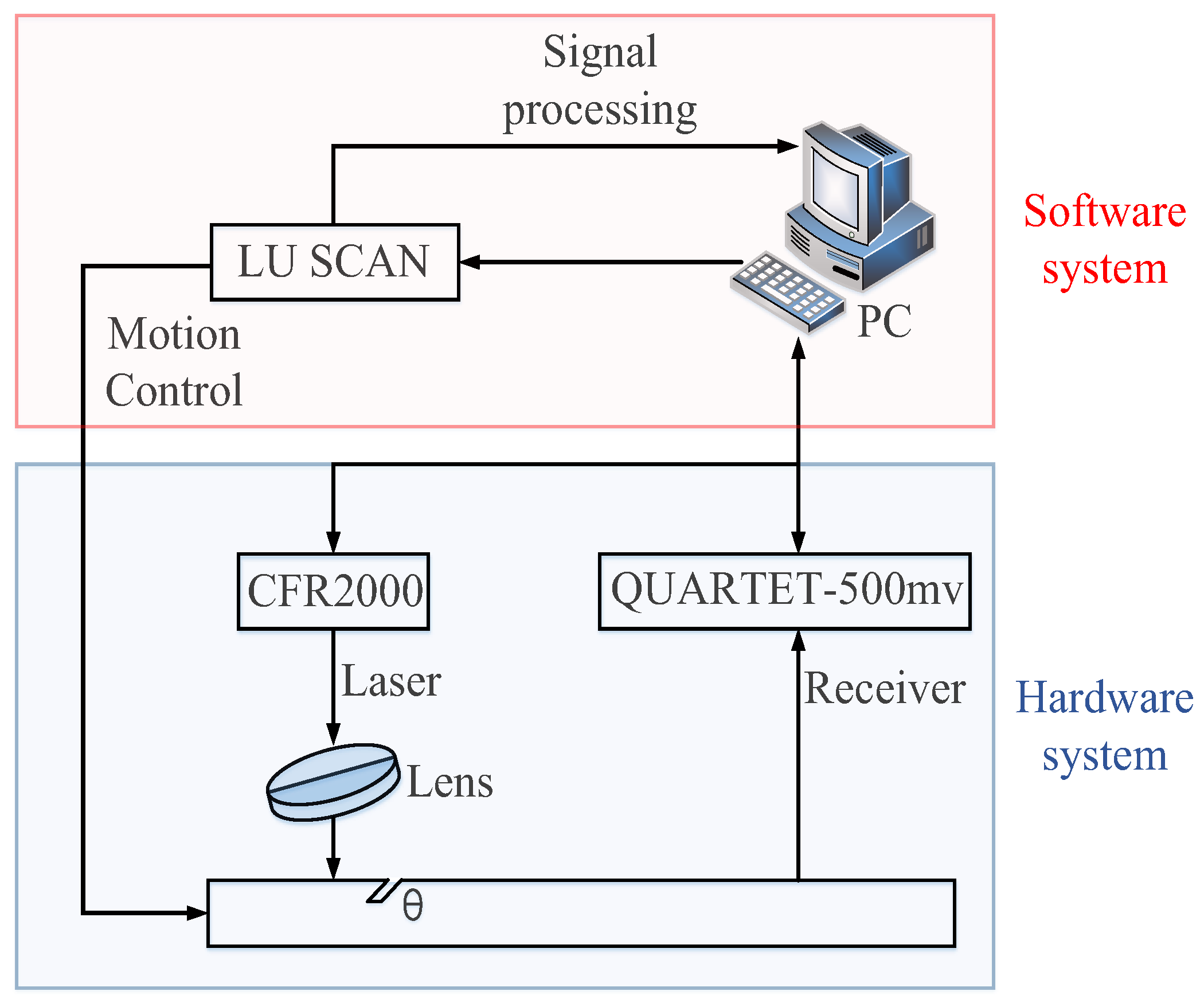
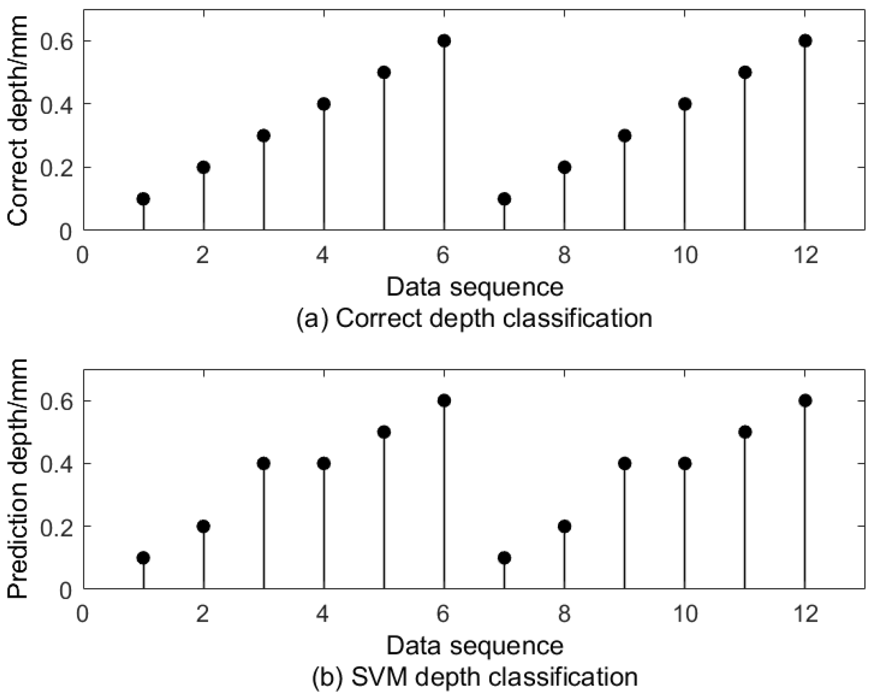
An intelligent detection method using the SVM model is provided by both FEM simulations and the experimental method. When putting the model established in this paper into actual detection, its accurate classification rates are 95.5% for angles and 83.3% for depths, which demonstrates the feasibility of the SVM model based on laser ultrasonics for practical surface crack detection.

References

1. Guan, J.; Shen, Z.; Ni, X.; Wang, J.; Lu, J.; Xu, B. Numerical simulation of the reflected acoustic wave components in the near field of surface defects. J. Phys. D Appl. Phys. 2006, 39, 1237–1243. [Google Scholar] [CrossRef]
2. Zhong, Y.; Gao, X.; Luo, L.; Pan, Y.; Qiu, C. Simulation of Laser Ultrasonics for Detection of Surface-Connected Rail Defects. J. Nondestruct. Eval. 2017, 36, 70. [Google Scholar]
3. Jian, X.; Fan, Y.; Edwards, R.S.; Dixon, S. Surface-breaking crack gauging with the use of laser-generated Rayleigh waves. J. Appl. Phys. 2006, 100, 064907. [Google Scholar] [CrossRef]
4. Edwards, R.; Dixon, S.; Jian, X. Characterisation of defects in the railhead using ultrasonic surface waves. NDT E Int. 2006, 39, 468–475. [Google Scholar] [CrossRef]
5. Zhou, Z.; Zhang, K.; Zhou, J.; Sun, G.; Wang, J. Application of laser ultrasonic technique for non-contact detection of structural surface-breaking cracks. Opt. Laser Technol. 2015, 73, 173–178. [Google Scholar] [CrossRef]
6. Li, H.; Pan, Q.; Zhang, X.; An, Z. An Approach to Size Sub-Wavelength Surface Crack Measurements Using Rayleigh Waves Based on Laser Ultrasounds. Sensors 2020, 20, 5077. [Google Scholar] [CrossRef]
7. Shakibi, B.; Honarvar, F.; Moles, M.; Caldwell, J.; Sinclair, A.N. Resolution enhancement of ultrasonic defect signals for crack sizing. NDT E Int. 2012, 52, 37–50. [Google Scholar] [CrossRef]
8. Yi, Q.; Wang, H.; Guo, R.; Li, S.; Jiang, Y. Laser ultrasonic quantitative recognition based on wavelet packet fusion algorithm and SVM. Optik 2017, 149, 206–219. [Google Scholar] [CrossRef]
9. Zhang, Y.; Wang, X.; Yang, Q.; Dong, F.; Du, X.; Yin, A. Characterization of mean grain size of interstitial-free steel based on laser ultrasonic. J. Mater. Sci. 2018, 53, 8510–8522. [Google Scholar] [CrossRef]
10. Liu, X.; Yang, S.; Liu, Y. Numerical Study for Surface-breaking Crack Detection on a Cylinder Using Laser-generated Ultrasound. In Proceedings of the 2018 15th International Conference on Ubiquitous Robots (UR), Jeju, Korea, 28 June–1 July 2018; pp. 797–802. [Google Scholar]
11. Li, K.; Ma, Z.; Fu, P.; Krishnaswamy, S. Quantitative evaluation of surface crack depth with a scanning laser source based on particle swarm optimization-neural network. NDT E Int. 2018, 98, 208–214. [Google Scholar] [CrossRef]
12. Li, K.; Sui, H.; Dong, X.; Gao, L.; Gao, H. Intelligent Evaluation of Crack detection with Laser Ultrasonic technique. IOP Conf. Ser. Earth Environ. Sci. 2020, 514, 022014. [Google Scholar] [CrossRef]
13. Shukla, K.; Di Leoni, P.C.; Blackshire, J.; Sparkman, D.; Em Karniadakis, G. Physics-Informed Neural Network for Ultrasound Nondestructive Quantification of Surface Breaking Cracks. J. Nondestruct. Eval. 2020, 39, 61. [Google Scholar] [CrossRef]
14. Chen, Y.; Ma, H.-W.; Zhang, G.-M. A support vector machine approach for classification of welding defects from ultrasonic signals. Nondestruct. Test. Eval. 2014, 29, 243–254. [Google Scholar] [CrossRef]
15. Cortes, C.; Vapnik, V. Support-vector networks. Mach. Learn. 1995, 20, 273–297. [Google Scholar] [CrossRef]
16. Liu, Z.; Cui, Y.; Li, W. A Classification Method for Complex Power Quality Disturbances Using EEMD and Rank Wavelet SVM. IEEE Trans. Smart Grid 2015, 6, 1678–1685. [Google Scholar] [CrossRef]
17. Bai, X.; Wang, W. Principal pixel analysis and SVM for automatic image segmentation. Neural Comput. Appl. 2016, 27, 45–58. [Google Scholar] [CrossRef]
18. Matz, V.; Kreidl, M.; Smid, R. Classification of ultrasonic signals. Int. J. Mater. Prod. Technol. 2006, 27, 145–155. [Google Scholar] [CrossRef]
19. Yadavar Nikravesh, S.M.; Hossein, R.; Margaret, K.; Hossein, T. Intelligent Fault Diagnosis of Bearings Based on Energy Levels in Frequency Bands Using Wavelet and Support Vector Machines (SVM). J. Manuf. Mater. Processing 2019, 3, 11. [Google Scholar] [CrossRef]
20. Virmani, J.; Kumar, V.; Kalra, N.; Khandelwal, N. SVM-Based Characterization of Liver Ultrasound Images Using Wavelet Packet Texture Descriptors. J. Digit. Imaging 2013, 26, 530–543. [Google Scholar] [CrossRef] [PubMed]
21. Jiang, Y.; Wang, H.; Tian, G.; Yi, Q.; Zhao, J.; Zhen, K. Fast classification for rail defect depths using a hybrid intelligent method. Optik 2018, 180, 455–468. [Google Scholar] [CrossRef]
Figure 1. SVM system flow chart.
Applsci 12 08124 g001
Figure 2. Geometry of the FEM model.
Applsci 12 08124 g002
Figure 3. (a) Function in the time domain; (b) function in the spatial domain.
Applsci 12 08124 g003
Figure 4. Laser ultrasonic propagation images. (a) t = 1.33 μs. (b) t = 3.34 μs.
Applsci 12 08124 g004
Figure 5. Laser ultrasonic direct wave and transmitted wave displacement waveform. (a) Reflected wave. (b) Transmitted wave.
Applsci 12 08124 g005aApplsci 12 08124 g005b
Figure 6. Feature extraction flowchart. X: WP coefficient peak; Y: WP energy peak; Z: WP entropy.
Applsci 12 08124 g006
Figure 7. Three-dimensional map of the angle–depth–transmitted wave peak.
Applsci 12 08124 g007
Figure 8. Three-dimensional map of the angle–depth–root mean square.
Applsci 12 08124 g008
Figure 9. 3D map of the depth-angle-transmission coefficient.
Applsci 12 08124 g009
Figure 10. 3D map of the angle–depth–reflection coefficient.
Applsci 12 08124 g010
Figure 11. 3D map of depth and angle versus deconvolution sum.
Applsci 12 08124 g011
Figure 12. (a) Scatter plot of WP coefficient peaks; (b) scatter plot of WP energy peaks; (c) scatter plot of WP entropy.
Applsci 12 08124 g012aApplsci 12 08124 g012b
Figure 13. (a) Scatter plot of the root mean squares of reflected waves. (b) Scatter plot of transmission coefficients.
Applsci 12 08124 g013aApplsci 12 08124 g013b
Figure 14. (a) SVM prediction error with the root mean square of the Rr wave; (b) SVM prediction error with transmission coefficient.
Applsci 12 08124 g014
Figure 15. SVM prediction error differences between A and B.
Applsci 12 08124 g015
Figure 16. Three-dimensional map of depth and angle versus feature parameter.
Applsci 12 08124 g016
Figure 17. (a,b) depth sequence; (c,d) angle sequence.
Applsci 12 08124 g017
Figure 18. SVM depth prediction errors.
Applsci 12 08124 g018
Figure 19. SVM angle prediction errors.
Applsci 12 08124 g019
Figure 20. Schematic block diagram of the experimental platform.
Applsci 12 08124 g020
Figure 21. Three- and two-dimensional plots of the B-Scan image of oblique cracks (angle = 60°, depth = 0.5 mm).
Applsci 12 08124 g021
Figure 22. Initial signal and denoising signal of the Rr wave.
Applsci 12 08124 g022
Figure 23. Initial signal and denoising signal of the Tr wave.
Applsci 12 08124 g023
Figure 24. Experimental data and fitting line of the normalized feature parameter versus angles.
Applsci 12 08124 g024
Figure 25. Experimental data and fitting line of the normalized feature parameter versus depth.
Applsci 12 08124 g025
Figure 26. (a) Actual angle sequence; (b) prediction angle sequence.
Applsci 12 08124 g026
Figure 27. (a) Actual depth sequence; (b) prediction depth sequence.
Applsci 12 08124 g027
Figure 28. (a,b) prediction errors.
Applsci 12 08124 g028