Article

Evolution Law of Three-Dimensional Non-Uniform Temperature Field of Tunnel Construction Using Local Horizontal Freezing Technique

1
School of Civil Engineering and Architecture, Anhui University of Science and Technology, Huainan 232001, China
2
School of Architectural Engineering, Nantong Vocational University, Nantong 226007, China
*
Author to whom correspondence should be addressed.
Appl. Sci. 2022, 12(16), 8093; https://doi.org/10.3390/app12168093
Submission received: 7 July 2022 / Revised: 9 August 2022 / Accepted: 9 August 2022 / Published: 12 August 2022
(This article belongs to the Special Issue Artificial Ground Freezing Technology)

Abstract

:
The formation quality of a frozen wall is one of the prerequisites for tunnel excavation using artificial ground freezing techniques. However, the non-uniformity of temperature distribution along the length direction of the freezing pipe is often ignored in the actual freezing engineering, which leads to a thin frozen wall at a local position that does not meet the design requirements. Therefore, exploring the evolution law of three-dimensional non-uniform freezing temperature fields is necessary. In this paper, a tunnel horizontal freezing model test system was established based on the similarity criterion of hydro–heat coupling, and the temperatures at three sections were tested using thermocouple temperature sensors. The results show that the temperature drop curves of measurement points suffer from three periods: steep drop, slow drop and tending to be stable. The temperature curves on the main and vice planes of the frozen wall all present a “V” type; specifically, the temperature on the axis plane is the lowest, while the temperature away from the axis plane is higher, and the temperature gradient outside the axis plane is greater than that inside. The frozen wall develops from frozen soil columns to a sector ring, and the average thickness of the frozen wall at three sections is 50.6, 40.7 and 75.1 mm after freezing for 60 min, respectively, which shows an obvious non-uniformity. The temperature distribution along the length of the freezing pipe is T = −0.000045z2 + 0.0205z − 13.5125. The freezing temperature contours calculated by ABAQUS are basically consistent with those calculated by the model test after calling the temperature function of the freezing pipe wall.

1. Introduction

Artificial ground freezing techniques, used as ground reinforcement methods that freeze pore water into ice to form an impermeable layer, have the advantages of good water sealing, high strength and stiffness, strong adaptability, green environmental protection and so on, so they are widely used in underground engineering. In freezing construction, it is very important to master the thickness of the frozen wall, which depends on the distribution of the freezing temperature field. Thus, exploring the evolution law of the freezing temperature field is the foundation of tunnel construction using artificial ground freezing techniques [1,2]. Scholars’ research achievements through the following three methods are mainly as follows:
(1)
Theoretical analysis: Trupak [3] and Bakholdin [4] presented the calculation methods of single-piped, single-circle-piped and double-circle-piped steady-state freezing temperature fields. Subsequently, Sanger and Sayles [5,6] optimized the analytical solution of a single-circle-piped freezing temperature field. On this basis, Tobe [7] derived an analytical solution for a multi-circle-piped freezing temperature field, and then Hu [8,9,10,11,12] optimized these analytical solutions. In addition, Aziz [13], Hosseini [14], Jiji [15], Jiang [16] and Cai [17] derived the analytical solution of a single-piped transient freezing temperature field.
(2)
Numerical simulation: Yang [18], Yu [19,20], Fu [21] and Cai [22] studied the distribution law of the freezing temperature field of a subway connecting passage by different finite element software. Hong [23] studied the evolution law of the local horizontal freezing temperature field of an underground tunnel with a shallow depth by ABAQUS. Hu [24] studied the distribution law of the cup-type freezing temperature field of the tunnel port and found that the closure of outer-circle pipes was earlier than that of inner-circle pipes.
(3)
Model tests: Shang [25] established a rectangular tunnel construction model and found that the outer edge of the frozen wall developed slowly due to the heat dissipation of the model surface. Shi [26] established a shield docking freezing model and determined the positive freezing time. Cai [27] and Duan [28] established a pipe-roof freezing model with different types of freezing pipe and found that the freezing effect of an empty pipe with a double circular freezer was the best. Zhang [29] established a tunnel vertical freezing model and found that the thickness of the basin-type frozen wall upstream was smaller than that downstream.
None of the above studies consider the loss of cooling capacity along the length direction of the freezing pipe, which leads to the three-dimensional non-uniformity of the freezing temperature field in actual engineering. In this paper, a tunnel horizontal freezing model test system was established based on the similarity theory to explore the evolution law of the three-dimensional non-uniform transient temperature field of construction of an underground tunnel using the local horizontal freezing method.

2. Model Test Design

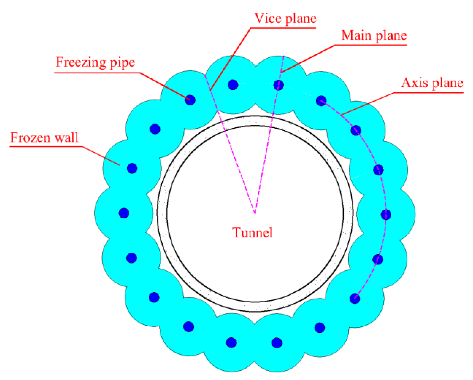
2.1. Project Overview

A local horizontal freezing project is located south of the section between the Dabeiyao and thermal power plant section of the Beijing Metro Fu-ba line [23]. The buried depth of this tunnel is 10 m, and the maximum excavation diameter is 3.0 m. A 1.2 m-thick freezing mild clay layer at the arch of the tunnel was formed through 8 freezing pipes with an outer diameter of 108 mm. There are some long-term disrepaired sewage pipelines over the tunnel, and the downward seepage is serious. The mild clay layer is in a saturated state all year round, and soil mass moisture content can reach 21.72%.

2.2. Derivation of Similarity Criteria

The heat conduction differential equation of soil freezing is as follows:
θ n τ = a n ( 2 θ n r 2 + 1 r θ n r )   ( 0 < r 0 < r < ,   τ > 0 ,   n = 1   ,   2 )
where r is radial coordinate, e is time; θ is soil temperature, which is the temperature of unfrozen area when n = 1 and that of frozen area when n = 2 , r 0 is the outer radius of freezing pipes, and a is the thermal diffusivity of soil.
The initial and boundary conditions of soil freezing temperature field [30] are
{ θ ( r , 0 ) = θ 0 θ ( , τ ) = θ 0 θ ( ρ , τ ) = θ f θ ( r 0 , τ ) = θ y
where θ 0 is the initial temperature of soil, ρ is the external surface coordinates of frozen wall, θ f is the freezing temperature of soil, θ y is the wall temperature of freezing pipes.
The heat balance equation at the freezing front ( r = ρ ) is
λ 2 θ 2 r | r = ρ λ 1 θ 1 r | r = ρ = L d ρ d τ
where λ is the thermal conductivity of soil, L is the latent heat of soil.
According to Equations (1)–(3), the similarity criterion equation of soil freezing temperature field can be obtained by equation analysis method.
F ( F 0 , K 0 , R , θ ) = 0
where F 0 = a τ r 2 is the Fourier criterion of temperature field; K 0 = L c θ is Kosović criterion and c is the specific heat of soil; R is geometric criterion, and θ is temperature criterion.
In the model test, the soil was taken from the site, C ρ = 1 , C a = 1 , C c = 1 , C L = 1 . The water content of soil is the same, so the latent heat released during freezing is equal, which is substituted into Equation (4) to obtain:
C τ = C r 2
C θ = 1
Equation (5) shows that the time similarity ratio in the model test is the square of the geometric similarity ratio; according to Equation (6), the temperature of each point in the model test is the same as that of each corresponding point in the prototype.
Water migration occurs in the soil freezing process, and its essence is the humidity field problem in the freezing process. The mathematical model is:
h τ = b ( 2 h r 2 + 1 r h r )
The boundary condition is:
{ h ( r , 0 ) = h 0 h ( , τ ) = h 0 h ( ρ , τ ) = 0
where h is humidity, and b is moisture conductance.
According to Equations (7) and (8), the similarity criterion equation of soil moisture field can be obtained by the equation analysis method as follows:
F ( F h , R , H ) = 0
where F h = b τ r 2 is the Fourier criterion of humidity field, H is humidity criterion.
It shows that the water transfer process and soil freezing process are similar in the mathematical model, and they all obey the Fourier criterion. Therefore, under the condition of geometric similarity, as long as the temperature field is similar, the humidity field is also similar to the temperature field.
In this paper, the similarity ratio of geometry ( C l ) in the model test was determined to be 30; this ratio can be used to calculate the similarity ratio of other parameters (Table 1) according to the aforementioned similarity criteria.
In Table 1, the similarity ratio is the ratio of the value of the same physical quantity in the prototype to that in the model; that is, the size will be reduced by 30 times and time will be reduced by 900 times in the model test, while temperature, humidity (soil moisture), density, thermal conductivity, specific heat and latent heat of phase change remain consistent with those in the prototype.

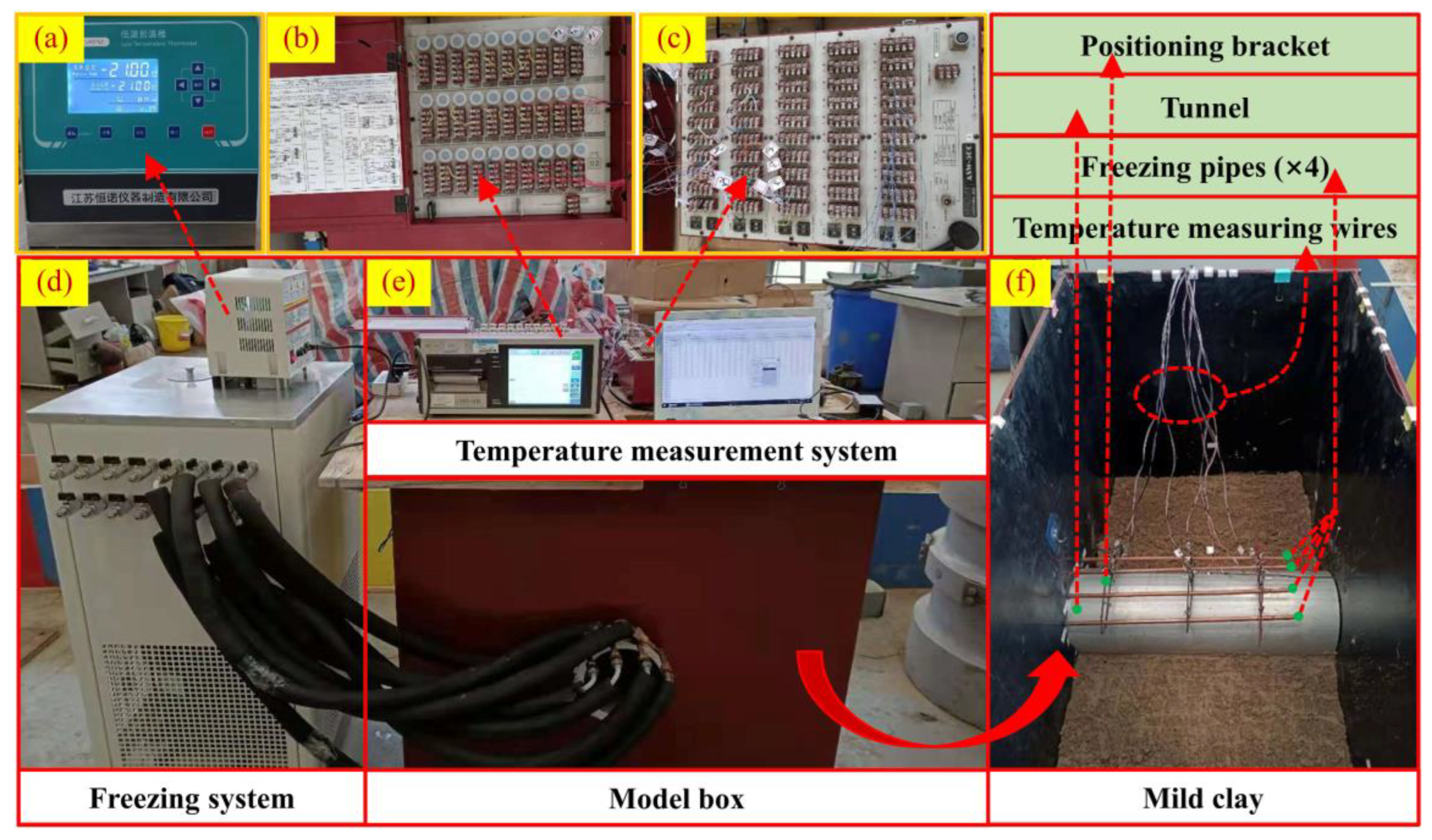
2.3. Model Test System

Figure 1 shows the tunnel horizontal freezing model test system, which includes a model box, freezing system and temperature measurement system.
(1)
Model box
The size of the model box in Figure 2e was 1000 mm × 800 mm × 700 mm, and freezing pipes in Figure 2f were set horizontally along the width direction of the box. The parameters of mild clay are shown in Table 2.
(2)
Freezing system
As shown in Figure 2a,d, the freezing equipment adopted the low-temperature thermostat produced by Jiangsu Hengnuo Instrument Manufacturing Co., Ltd. (Nanjing, China), which allowed alcohol to maintain a temperature of −21 °C for cycle operation. The test time was set as 72 min, where the positive time was 60 min, and the design thickness of the frozen wall was set as 40 mm. In this model test, 4 freezing pipes with an outer diameter of 8 mm were determined by the equivalent heat transfer and similarity criteria, and these pipes were symmetrically distributed above the tunnel at an angle of 28°. The structure of the freezing pipe is a coaxial sleeve, and the circulation mode of alcohol is entering from the inner pipe and leaving from the outer pipe, and its flow rate is 1.2 m3/h, as shown in Figure 3.
(3)
Temperature measurement system
A TDS-630 multi-point data acquisition instrument in Figure 2b,c was selected to record temperature, and the acquisition frequency was set as 1 min/time. In this model test, three temperature measurement sections were set along the length direction of the freezing pipe, that was 50 mm, 250 mm and 450 mm from the orifice of the freezing pipe. At each temperature measurement section, there were 23 measurement points in the soil and 4 measurement points on the freezing pipe wall, as shown in Figure 3.

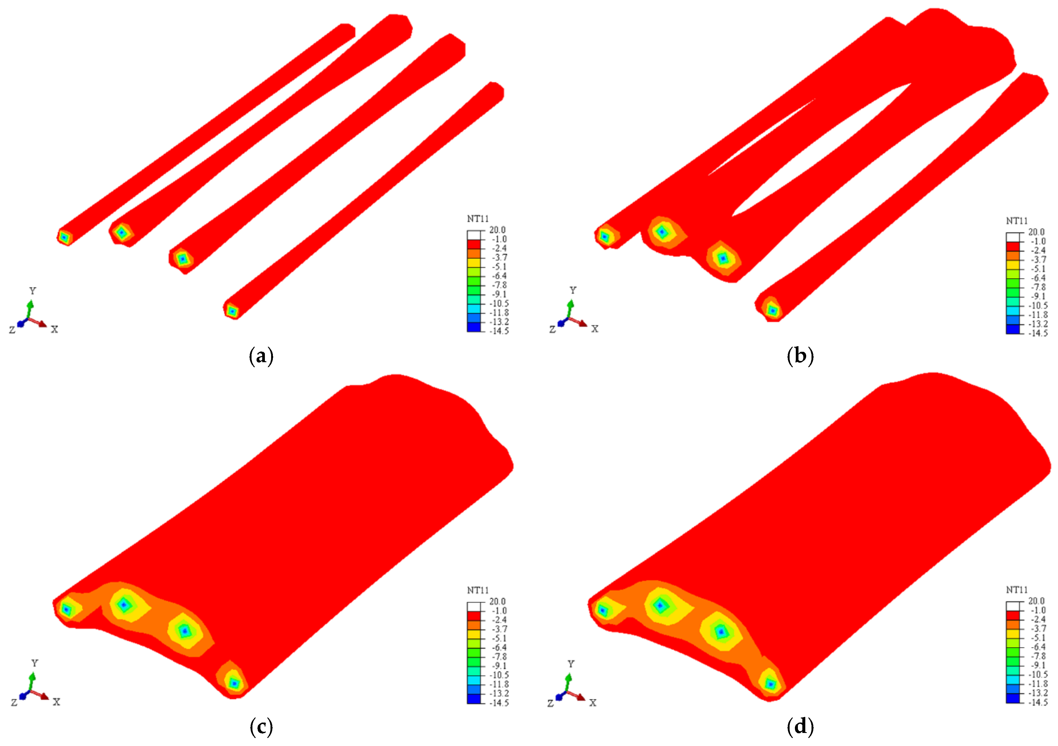
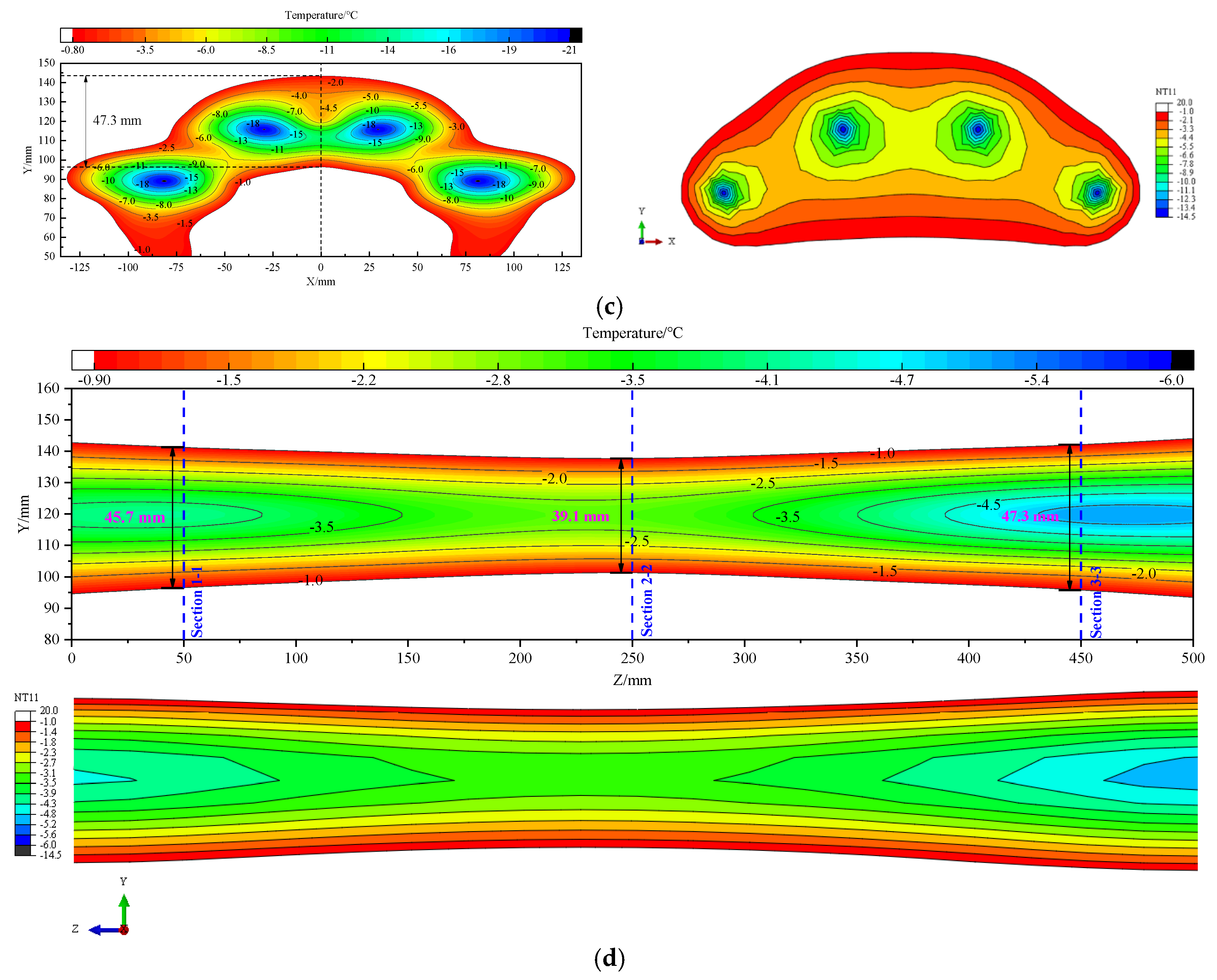
3. Model Test Results

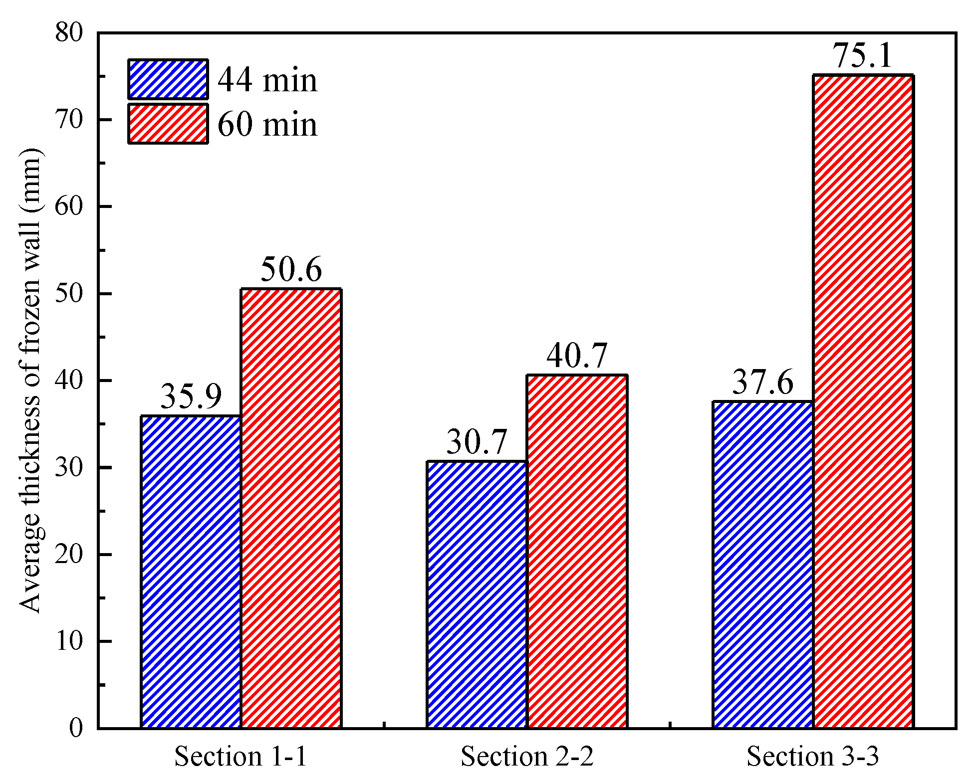
3.1. Temperature Variation Analysis

The temperature duration curves of each measurement point at three sections in the model test are shown in Figure 4.
Figure 4 shows that the temperature drop curves of the measurement points suffer from three periods: steep drop, slow drop and tending to be stable. The temperature of the measurement point between the adjacent two freezing pipes decreases faster, while that outside the freezing pipe decreases slower. Figure 4a shows that the temperatures of measurement points are all below –1 °C after freezing for 55 min. The temperature drop rates of measurement point ⑪ are 0.365, 0.182 and 0.024 °C/min at three periods; Figure 4b shows that the temperatures of measurement points are all below –1 °C after freezing for 70 min. The temperature drop rates of measurement point ⑪ are 0.318, 0.120 and 0.011 °C/min at three periods; Figure 4c shows that the temperatures of measurement points are all below –1 °C after freezing for 60 min. The temperature drop rates of measurement point ➅ are 0.334, 0.148 and 0.019 °C/min at three periods.

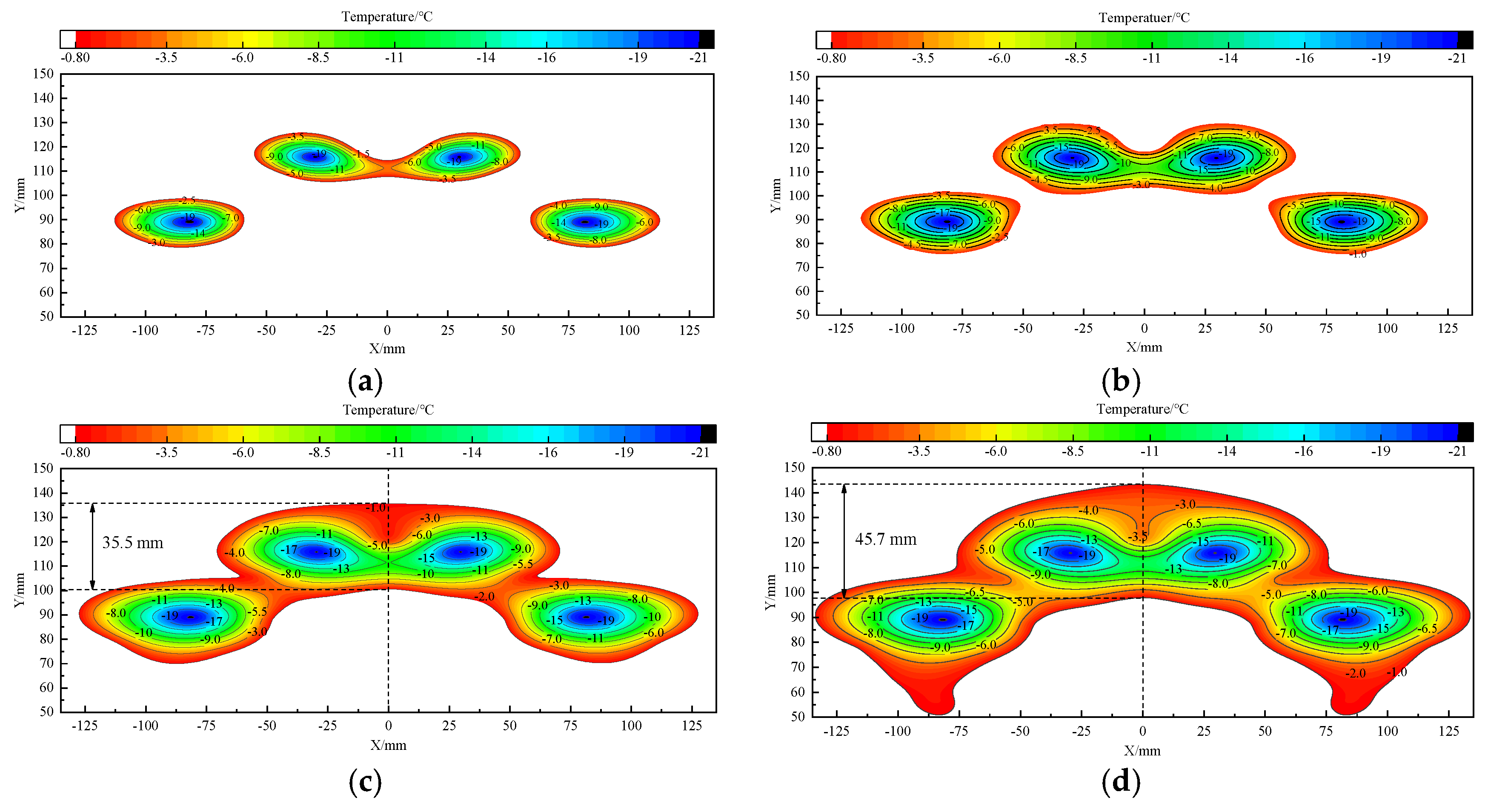
3.2. Temperature Field Evolution Perpendicular to Freezing Pipes

The freezing temperature fields at three sections are shown in Figure 5, Figure 6 and Figure 7 after freezing for 4 min, 28 min, 44 min and 60 min.
Figure 5, Figure 6 and Figure 7 show that after freezing for 4 min, a circular frozen soil column is formed around the freezing pipes. After freezing for 28 min, the diameter of the frozen soil columns further expands, the two frozen soil columns in the middle intersect first. After freezing for 44 min, the frozen wall basically intersects, the thickness of the frozen wall at the tunnel arch in three sections is 35.5 mm, 18.9 mm and 32.7 mm, respectively. After freezing for 60 min, the frozen wall completely intersects, and the thickness of the frozen wall at the tunnel arch in three sections is 45.7 mm, 39.1 mm and 47.3 mm, respectively. Moreover, the freezing temperature field can be calculated by the single pipe freezing theory within freezing for 28 min, while it can be calculated by the flat-panel freezing theory [31] after freezing for 28 min. After freezing for 60 min, the order of the freezing effect is Section 3-3 > Section 1-1 > Section 2-2.
To quantitatively analyze the non-uniformity of temperature distribution at three sections, the temperature on two characteristic planes (the main and vice planes) of the horizontal frozen wall are selected to draw curves. Where the main plane refers to the characteristic plane passing through the center of the tunnel and each freezing pipe, the vice plane refers to the characteristic plane passing through the center of the tunnel and the midpoint of the connecting line between adjacent freezing pipes, while the axis plane refers to the arrangement circle of freezing pipes, as shown in Figure 8.
Figure 9, Figure 10 and Figure 11 show that the temperature curves on the main and vice planes of the frozen wall present a “V” type; specifically, the temperature on the axis plane is the lowest, while it gradually rises with the increase in distance to the axis plane. Moreover, the temperature curve near the inner and outer edges (R = 100 mm and R = 140 mm) of the designed frozen wall tends to be flat, and the temperature at the inner edge (R = 100 mm) is always lower than that at the outer edge (R = 140 mm) during freezing for 60 min. It indicates that the dissipation capacity of the cooling capacity inside the axis plane of the frozen wall is less than that outside the axis plane.
In addition, at the early stage of freezing, the temperature drop rate inside the axis plane is bigger than that outside the axis plane. At Section 1-1, along the main plane, the average temperature drop rate outside the axis plane is approximately 0.254 °C/min, while it is approximately 0.259 °C/min inside the axis plane. Meanwhile, along the vice plane, the average temperature drop rate outside the axis plane is approximately 0.252 °C/min, while it is approximately 0.254 °C/min inside the axis plane. At the later stage of freezing, the temperature drop rate inside and outside the axis plane is roughly the same.
The duration curves of the average temperature gradient of the frozen wall at three sections are shown in Figure 12.
Figure 12 shows that the average temperature gradient at the inside and outside of the frozen wall first increases, then decreases and finally tends to be stable with the increase in freezing time. At Section 1-1, after freezing for 4 min, the average temperature gradient outside the axis plane is only 0.07 °C/mm, while it is 0.05 °C/mm inside the axis plane. After freezing for 28 min, the average temperature gradient outside the axis plane is only 0.446 °C/mm, while it is 0.395 °C/mm inside the axis plane. After freezing for 44 min, the average temperature gradient outside the axis plane is only 0.325 °C/mm, while it is 0.311 °C/mm inside the axis plane. After freezing for 60 min, the average temperature gradient outside the axis plane is only 0.288 °C/mm, while it is 0.280 °C/mm inside the axis plane. It is obvious that the average temperature gradient on the outside of the frozen wall is more than that on the inside of the frozen wall. Moreover, the order of the value of the average temperature gradient at three sections is Section 3-3 > Section 2-2 > Section 1-1.

3.3. Temperature Field Evolution Parallel to Freezing Pipes

The temperature field parallels to the freezing pipe at the tunnel vertical center line after positive freezing for 60 min is shown in Figure 13.
Figure 13 shows the morphology of the frozen wall, which is thicker at the ends and thinner in the middle; it is intuitive and obvious that the frozen wall is non-uniform. The average thickness of the frozen wall at three sections after positive freezing for 44 and 60 min is shown in Figure 14.
Figure 14 shows that the average thickness of the frozen wall at three sections is not all equal after freezing for 44 min and 60 min. After freezing for 44 min, the average thickness of the frozen wall at Sections 1-1, 2-2 and 3-3 is 35.9 mm, 30.7 mm and 37.6 mm, respectively; after freezing for 60 min, the average thickness of the frozen wall at Sections 1-1, 2-2 and 3-3 is 50.6 mm, 40.7 mm and 75.1 mm, respectively. The order of the average thickness of the frozen wall at three sections is Section 3-3 > Section 1-1 > Section 2-2, which presents the non-uniformity of a frozen wall along the length direction of the freezing pipe.
The pipe wall temperature fitting curves along the length direction of the freezing pipe are shown in Figure 15 after freezing for 4 min, 28 min, 44 min and 60 min.
Figure 15 shows that the pipe wall temperature first increases and then decreases along the length direction of the freezing pipe, where it reaches the maximum at Section 2-2. After freezing for 4 min, 28 min, 44 min and 60 min, the temperature fitting functions are as follows:
{ T = 0.00015625 z 2 + 0.06138 z + 14.92187 T = 0.00005 z 2 + 0.0215 z 11.55 T = 0.0000425 z 2 + 0.01725 z 12.25625 T = 0.000045 z 2 + 0.0205 z 13.5125 t = 4 min t = 28 min t = 44 min t = 60 min
The conclusion obtained from the model test is inconsistent with the common sense that the alcohol temperature in the outer pipe gradually rises from the distal end to the proximal end of the freezing pipe; the main reason lies in the structure of the freezing pipe. As shown in Figure 16, the freezing pipe used in this model test is composed of an outer pipe, an inner pipe and a three-pipe joint; it is also commonly used in practical engineering. The low-temperature alcohol enters from the inner pipe, flows through the inner pipe to the end of the freezing pipe, and then flows back to the three-pipe joint through the outer pipe. When the alcohol flows in the outer pipe, it indirectly cools the soil by absorbing the heat transferred by the soil to the pipe wall, so as to achieve the purpose of freezing soil. Usually, the temperature of the pipe wall should gradually rise along the flow direction of the alcohol in the outer pipe, and the temperature of the pipe wall on each section should be shown as Section 3-3 < Section 2-2 < Section 1-1. However, the alcohol flowing in the outer pipe not only has heat exchange with the outer pipe wall, but also has heat exchange with the inner pipe wall, and there is also heat exchange between the inner pipe wall and the alcohol flowing in the inner pipe. The complex heat exchange process eventually leads to the non-uniform distribution of the temperature of the outer pipe wall of the freezing pipe, and the specific thermodynamic theory needs further study.

4. Numerical Simulation Design

4.1. Establishment of Model

The numerical simulation can more intuitively unfold the development process of the frozen wall. Based on the pipe wall temperature fitting function calculated by the model test, a three-dimensional finite element model is established to simulate the freezing temperature field, as shown in Figure 17.
Figure 17 shows that the model size is 1000 mm × 800 mm × 500 mm. The element type is DC3D8 with good heat-transfer capability, and the number of elements is 59120, where the four freezing pipes are simplified as linear heat sources, and each freezing pipe consists of 25 linear elements.

4.2. Boundary Conditions

The initial temperature of soil elements is set as 20 °C, while the temperature of line elements of the freezing pipe is set as the temperature fitting function.

4.3. Material Parameters

The soil elements are given the material parameters of mild clay, as shown in Table 2.

5. Numerical Simulation Results

The validation of the numerical simulation results with model test results at temperature measuring point ⑪ at Section 3-3, which has a good representative, is shown in Figure 18.
As shown in Figure 18, the numerical simulation results are basically consistent with the model test results; the two curves both show a change process of steep drop first, then slow drop and finally stabilized. The difference between them mainly occurs at the steep drop stage, where the model test results are always lower than the numerical simulation results, and the maximum reaches 2.5 °C. The difference in refrigerating capacity may be due to the unstable ambient temperature in the laboratory or the influence of some unpredictable factors; that is, the model test results may have errors in reflecting the development of freezing temperature field. In contrast, the numerical simulation results can reflect the development of the freezing temperature field more reasonably.
The evolution law of the three-dimensional freezing temperature field is shown in Figure 19 after freezing for 4 min, 28 min, 44 min and 60 min.
Figure 19 shows that the three-dimensional freezing temperature field has obvious non-uniformity after freezing for 4 min, 28 min, 44 min and 60 min. The frozen walls at both ends of the freezing pipe connect at first, and the frozen walls in the middle of the freezing pipe connect subsequently. After freezing for 4 min, four independent frozen soil columns are formed with the characteristic that both ends are coarser and the middle is thinner. After freezing for 28 min, the two frozen soil columns in the middle connect in turn at Section 3-3 and Section 1-1, then expand along with the negative and positive directions of freezing depth, respectively, and eventually converge at Section 2-2. During this period, the frozen soil columns on both sides also gradually develop following this law. After freezing for 48 min, the frozen wall basically intersects, and the whole frozen wall still presents the law that is thin in the middle and thick at both ends. After freezing for 60min, the frozen wall completely intersects, and the thickness of the frozen wall meets the design requirements.
The comparison of the freezing temperature field calculated by numerical simulation and model test is shown in Figure 20 after freezing for 60 min.
Figure 20 shows that after freezing for 60 min, the thickness of the frozen wall at three sections is different; that is, the thickness of Section 1-1, 2-2 and 3-3 at tunnel arch is 45.7 mm, 39.1 mm and 47.3 mm in the model test, while it is 46.3 mm, 40.9 mm and 49.4 mm in the numerical simulation, respectively. The difference between them is 0.6 mm, 1.8 mm and 2.1 mm, and no matter the sections perpendicular or parallel to the length direction of the freezing pipes, the shapes of the frozen wall at each section are all basically consistent in the numerical simulation and the model test, which indicates that the numerical simulation method has high prediction accuracy after introducing the temperature fitting function of the freezing pipe wall.

6. Conclusions

In this paper, the evolution law of a three-dimensional non-uniform temperature field is analyzed by combining the physical model test and numerical simulation during the tunnel construction using a local horizontal freezing technique. The main conclusions are as follows:
The temperature drop curves of the measurement points suffer from three periods: steep drop, slow drop and tending to be stable, and the temperature of the measurement point between the adjacent two freezing pipes decreases faster, while that located outside the freezing pipes decreases slower.
The temperature curves on the main and vice planes of the frozen wall present a “V” type, specifically, and the temperature on the axis plane is the lowest, while it gradually rises with the increase in distance to the axis plane. The average temperature gradient at the inside and outside of the frozen wall first increases, then decreases and finally tends to be stable with the increase in freezing time.
After freezing for 60 min, the frozen wall presents an obvious non-uniformity along the length direction of the freezing pipe, and the thickness at Section 1-1, 2-2 and 3-3 at the tunnel arch is 45.7 mm, 39.1 mm and 47.3 mm, respectively, and the difference with the numerical simulation results is 0.6 mm, 1.8 mm and 2.1 mm, respectively, which indicates that the new numerical simulation method introducing the temperature fitting function of the freezing pipe wall has high accuracy in predicting the evolution law of the non-uniform temperature field.
The results of this study are helpful to understand the temperature field development of the soil around sleeve-type freezing pipes and can provide a certain reference for the design and construction of such freezing projects and other aspects of research. Next, research on the evolution law of non-uniform temperature fields in the whole process of freezing and thawing under complex formation conditions will be carried out, as well as its frost heave and thaw settlement effects.

Author Contributions

Data curation, R.H., M.L. and Z.Y.; Funding acquisition, H.C.; Writing—original draft, C.P. All authors have read and agreed to the published version of the manuscript.

Funding

This research was funded by the National Natural Science Foundation of China, grant number 51778004; Academic Funding for Top-notch Talents in University Disciplines (Majors) of Anhui Province, China, grant number gxbjZD10; Research on Graduate Science Project in Anhui Province, China, grant number YJS20210383; Graduate Innovation Fund Project of Anhui University of Science and Technology, grant number 2020CX2024; and Graduate Innovation Fund Project of Anhui University of Science and Technology, grant number 2022CX2047.

Data Availability Statement

The datasets generated and analyzed during the current study are available from the corresponding author upon reasonable request.

Acknowledgments

The authors would like to thank Fangxing Yao, Longfei Yang, Heyin Wang for the field data measurements.

Conflicts of Interest

The authors declare no conflict of interest.

References

  1. Li, S.Q.; Gao, L.X.; Chai, S.X. Significance and interaction of factors on mechanical properties of frozen soil. Rock Soil Mech. 2012, 33, 1173–1177. [Google Scholar]
  2. Hu, X.D.; Wu, Y.H.; Li, X.Y. A field study on the freezing characteristics of freeze-sealing pipe roof used in ultra-shallow buried tunnel. Appl. Sci. 2019, 9, 1532. [Google Scholar] [CrossRef]
  3. Trupak, N.G. The Freezing of Rock during Drilling; Ugliet Hizdat: Moscow, Russia, 1954. [Google Scholar]
  4. Bakholdin, B.V. Select the Best Ore Freezing Mode for Construction Purposes; State Press: Moscow, Russia, 1963. [Google Scholar]
  5. Sanger, F.J. Ground freezing in construction. J. Soil Mech. Found. Div. 1968, 94, 923–950. [Google Scholar] [CrossRef]
  6. Sanger, F.J.; Sayles, F.H. Thermal and rheological computations for artificially frozen ground construction. Dev. Geotech. Eng. 1979, 26, 311–337. [Google Scholar]
  7. Tobe, N.; Akimata, O. Temperature distribution formula in frozen soil and its application. Refrigeration 1979, 54, 3–11. [Google Scholar]
  8. Hu, X.D.; Chen, J.; Wang, Y.; Li, W.P. Analytical solution to steady-state temperature field of single-circle-pipe freezing. Rock Soil Mech. 2013, 34, 874–880. [Google Scholar]
  9. Hu, X.D.; Yu, J.Z.; Ren, H.; Wang, Y.; Wang, J.T. Analytical solution to steady-state temperature field for straight-row-piped freezing based on superposition of thermal potential. Appl. Therm. Eng. 2017, 111, 223–231. [Google Scholar] [CrossRef]
  10. Hu, X.D.; Fang, T.; Han, Y.T. Generalized analytical solution to steady-state temperature field of double-circle-piped freezing. J. China Coal Soc. 2017, 42, 2287–2294. [Google Scholar]
  11. Hu, X.D.; Fang, T.; Zhang, L.Y. Analytical solution to temperature distribution in frozen soil wall with wavy boundaries by single-row- and double-row-piped freezing. Cold Reg. Sci. Technol. 2018, 148, 208–228. [Google Scholar] [CrossRef]
  12. Hong, Z.Q.; Hu, X.D.; Fang, T. Analytical solution to steady-state temperature field of Freeze-Sealing Pipe Roof applied to Gongbei tunnel considering operation of limiting tubes. Tunn. Undergr. Space Technol. 2020, 105, 103571. [Google Scholar] [CrossRef]
  13. Aziz, A.; Lunardini, V.J. Perturbation techniques in phase change heat transfer. Appl. Mech. Rev. 1993, 46, 29–68. [Google Scholar] [CrossRef]
  14. Hosseini, S.M.; Akhlaghi, M.; Shaken, M. Transient heat conduction in functionally graded thick hollow cylinders by analytical method. Heat Mass Transfer. 2007, 43, 669–675. [Google Scholar] [CrossRef]
  15. Jiji, L.M.; Ganatos, P. Approximate analytical solution for one-dimensional tissue freezing around cylindrical cryoprobes. Int. J. Therm. Sci. 2009, 48, 547–553. [Google Scholar] [CrossRef]
  16. Jiang, B.S.; Wang, J.G.; Zhou, G.Q. Analytical calculation of temperature field around a single freezing pipe. J. China Univ. Min. Technol. 2009, 38, 463–466. [Google Scholar]
  17. Cai, H.B.; Xu, L.X.; Yang, Y.G.; Li, L.Q. Analytical solution and numerical simulation of the liquid nitrogen freezing-temperature field of a single pipe. AIP Adv. 2018, 8, 055119. [Google Scholar] [CrossRef]
  18. Yang, P.; Ke, J.M.; Wang, J.G.; Chow, Y.K.; Zhu, F.B. Numerical simulation of frost heave with coupled water freezing, temperature and stress fields in tunnel excavation. Comput. Geotech. 2006, 33, 330–340. [Google Scholar] [CrossRef]
  19. Yu, C.Y.; Lu, M.Y. Study on development characteristics of horizontal freezing temperature field in subway connecting passage. IOP Conf. Ser. Earth Environ. Sci. 2020, 619, 012086. [Google Scholar] [CrossRef]
  20. Yu, C.Y. Research on development law of horizontal freezing temperature field of complex curtain. IOP Conf. Ser. Mater. Sci. Eng. 2020, 780, 032029. [Google Scholar] [CrossRef]
  21. Fu, Y.; Hu, J.; Wu, Y.W. Finite element study on temperature field of subway connection aisle construction via artificial ground freezing method. Cold Reg. Sci. Technol. 2021, 189, 103327. [Google Scholar] [CrossRef]
  22. Cai, H.B.; Huang, Y.C.; Pang, T. Finite element analysis on 3D freezing temperature field in metro connected aisle construction. J. Railw. Sci. Eng. 2015, 12, 1436–1443. [Google Scholar]
  23. Hong, R.B.; Cai, H.B.; Li, M.K. Integrated prediction model of ground surface deformation during tunnel construction using local horizontal freezing technology. Arab. J. Sci. Eng. 2022, 47, 4657–4679. [Google Scholar] [CrossRef]
  24. Hu, J.; Yang, P. Numerical analysis of temperature field within large-diameter cup-shaped frozen soil wall. Rock Soil Mech. 2015, 36, 523–531. [Google Scholar]
  25. Shang, H.S.; Yue, F.T.; Shi, R.J. Model test of artificial ground freezing in shallow-buried rectangular cemented soil. Rock Soil Mech. 2014, 35 (Suppl. S2), 149–155+161. [Google Scholar]
  26. Shi, R.J.; Yue, F.T.; Zhang, Y.; Lu, L. Model test on freezing reinforcement for shield junction Part 1: Distribution characteristics of temperature field in soil stratum during freezing process. Rock Soil Mech. 2017, 38, 368–376. [Google Scholar]
  27. Cai, H.B.; Liu, Y.J.; Hong, R.B.; Li, M.K.; Wang, Z.J.; Ding, H.L. Model test and numerical simulation analysis on freezing effect of different freezers in freeze-sealing pipe-roof method. Geofluids 2022, 2022, 5350650. [Google Scholar] [CrossRef]
  28. Duan, Y.; Rong, C.X.; Cheng, H.; Cai, H.B.; Xie, D.Z.; Ding, Y.L. Model test of freezing temperature field of the freeze-sealing pipe roof method under different pipe arrangements. J. Glaciol. Geocryol. 2020, 42, 479–490. [Google Scholar]
  29. Zhang, J.X.; Qi, Y.; Yang, H.; Song, Y.W. Temperature field expansion of basin-shaped freezing technology in sandy pebble stratum of Beijing. Rock Soil Mech. 2020, 41, 2796–2813. [Google Scholar]
  30. Cai, H.B.; Li, P.; Wu, Z. Model test of liquid nitrogen freezing-temperature field of improved plastic freezing pipe. J. Cold Reg. Eng. 2020, 34, 04020001. [Google Scholar] [CrossRef]
  31. Cai, H.B.; Liu, Z.; Li, S.; Zheng, T.L. Improved analytical prediction of ground frost heave during tunnel construction using artificial ground freezing technique. Tunn. Undergr. Space Technol. 2019, 92, 103050. [Google Scholar] [CrossRef]
Figure 1. Three-dimensional diagram of model test system.
Applsci 12 08093 g001
Figure 2. Tunnel horizontal freezing model test system: (a) the control panel of low-temperature constant temperature bath; (b,c): TDS-630 multi-point data acquisition instrument; (d) low-temperature thermostat; (e) model box; (f) mild clay and freezing pipes in the model box.
Applsci 12 08093 g002
Figure 3. Temperature measurement points.
Applsci 12 08093 g003
Figure 4. Temperature variation curves of all measurement points at each section: (a) Section 1-1; (b) Section 2-2; (c) Section 3-3.
Applsci 12 08093 g004aApplsci 12 08093 g004b
Figure 5. Temperature field at Section 1-1: (a) 4 min; (b) 28 min; (c) 44 min; (d) 60 min.
Applsci 12 08093 g005
Figure 6. Temperature field at Section 2-2: (a) 4 min; (b) 28 min; (c) 44 min; (d) 60 min.
Applsci 12 08093 g006
Figure 7. Temperature field at Section 3-3: (a) 4 min; (b) 28 min; (c) 44 min; (d) 60 min.
Applsci 12 08093 g007
Figure 8. Characteristic planes of frozen wall.
Applsci 12 08093 g008
Figure 9. Temperature distribution on characteristic planes at Section 1-1: (a) main planes; (b) vice planes.
Applsci 12 08093 g009
Figure 10. Temperature distribution on characteristic planes at Section 2-2: (a) main planes; (b) vice planes.
Applsci 12 08093 g010
Figure 11. Temperature distribution on characteristic planes at Section 3-3: (a) main planes; (b) vice planes.
Applsci 12 08093 g011
Figure 12. Duration curve of average temperature gradient of frozen wall at three sections.
Applsci 12 08093 g012
Figure 13. The temperature field parallels to the freezing pipe at tunnel vertical center line.
Applsci 12 08093 g013
Figure 14. The average thickness of frozen wall at three sections.
Applsci 12 08093 g014
Figure 15. Pipe wall temperature fitting curves along the length direction of the freezing pipe.
Applsci 12 08093 g015
Figure 16. Diagram of freezing pipe structure.
Applsci 12 08093 g016
Figure 17. Three-dimensional finite element model.
Applsci 12 08093 g017
Figure 18. The validation of numerical simulation results with model test results.
Applsci 12 08093 g018
Figure 19. Evolution of three-dimensional freezing temperature field: (a) 4 min; (b) 28 min; (c) 44 min; (d) 60 min.
Applsci 12 08093 g019
Figure 20. Temperature contours of model test and numerical simulation after freezing for 60 min: (a) Section 1-1; (b) Section 2-2; (c) Section 3-3; (d) the section parallels the freezing pipe at tunnel vertical center line.
Applsci 12 08093 g020aApplsci 12 08093 g020b
Table 1. Similarity ratios.
ParameterSimilarity Ratio
Geometry (m)30
Time (s)900
Temperature (°C)1
Humidity (%)1
Density (kg/m3)1
Thermal conductivity (kcal·m−1·d−1·°C−1)1
Specific heat (kcal·kg−1·°C−1)1
Latent heat of phase change (kcal·kg−1)1
Table 2. Soil parameters.
ParameterDensity
/(kg/m3)
Thermal Conductivity
/(kcal/(m °C·d))
Specific Heat
/(kcal/(kg·°C))
Latent Heat of Phase Change
/(kcal/kg)
Freezing Temperature
/(°C)
Mild clayUnfrozen210023.000.3578.93−1
Frozen38.060.240
Publisher’s Note: MDPI stays neutral with regard to jurisdictional claims in published maps and institutional affiliations.

