Abstract
The existence of intra-class spectral variability caused by differential scene components and illumination conditions limits the improvement of endmember extraction accuracy, as most endmember extraction algorithms directly find pixels in the hyperspectral image as endmembers. This paper develops a quadratic clustering-based simplex volume maximization (CSVM) approach to effectively alleviate spectral variability and extract endmembers. CSVM first adopts spatial clustering based on simple linear iterative clustering to obtain a set of homogeneous partitions and uses spectral purity analysis to choose pure pixels. The average of the chosen pixels in each partition is taken as a representative endmember, which reduces the effect of local-scope spectral variability. Then an improved spectral clustering based on k-means is implemented to merge homologous representative endmembers to further reduce the effect of large-scope spectral variability, and final endmember collection is determined by the simplex with maximum volume. Experimental results show that CSVM reduces the average spectral angle distance on Samson, Jasper Ridge and Cuprite datasets to below 0.02, 0.06 and 0.09, respectively, provides the root mean square errors of abundance maps on Samson and Jasper Ridge datasets below 0.25 and 0.10, and exhibits good noise robustness. By contrast, CSVM provides better results than other state-of-the-art algorithms.
1. Introduction
Due to the limitation of spatial resolution and the complexity of ground object distribution, mixed pixels exist in hyperspectral images (HSIs) and reduce the accuracy of traditional pixel-level applications [1]. Therefore, it is necessary to perform hyperspectral unmixing for further analysis, which includes extracting pure pixels (endmembers) and determining the fractions of each endmember in pixels (abundance). The former is called endmember extraction, and the latter is called abundance estimation. Hyperspectral unmixing has been used in many fields to improve the related performance, such as subpixel target detection, precise land cover mapping and Earth change detection [2,3,4,5,6,7].
The mixing model is the basis for the research of hyperspectral unmixing, containing the linear spectral mixing model (LMM) and nonlinear spectral mixing model (NLMM) [8,9]. LMM assumes the photons arriving at the sensor interact with one ground object, so each mixed pixel is described as a linear combination of endmembers weighted by the corresponding abundance. As a matter of fact, the photons will go through multiple reflections and refractions between various ground objects, leading to NLMM. It has no fixed expression and needs to be determined for specific land cover class. Hence, LMM is utilized in most endmember extraction algorithms (EEAs) due to the simple structure and good performance, and it is also used in our work.
EEAs based on convex geometry are widely used in linear spectral unmixing. The pure pixel index (PPI) projects all pixels onto a set of vectors, and pixels that fall at the endpoints of these vectors the most are selected as endmembers [10]. Based on PPI, vertex component analysis (VCA) uses the orthogonal direction of the subspace spanned by the determined endmembers as projection axis, and pixels with the extreme value is taken as a new endmember [11]. N-FINDR works by finding the simplex with maximum volume in the space of the HSI, and pixels that constitute this simplex are regarded as endmembers [12]. As a variant of N-FINDR, the simplex growing algorithm (SGA) reduces the computational cost by including a process of growing simplexes one vertex at a time [13]. The alternating volume maximization (AVMAX) improves N-FINDR, using an alternating optimization strategy to pin down some convergence characteristics [14]. To enhance the noise robustness, the minimum volume simplex algorithm (MVSA) fits the minimum simplex volume to the data and reduces the effect of noise and outliers by imposing a hinge type soft constraint on the abundance [15]. The fast subspace-based module (FSPM) detects convex hull vertices for component pairs obtained by singular value decomposition and proposes a local outlier score measurement to remove outliers [16]. The statistics-based EEAs decompose the data into the product of endmember matrix and abundance matrix simultaneously, and iteratively solves the problem by adding prior constrained information. This type of method handles HSIs with a high mixing degree well but requires a lot of computations. The nonnegative matrix factorization (NMF) is a commonly used method. Based on NMF, several improved approaches have emerged by adding different constraints, such as minimum volume constrained NMF (MVC-NMF), -NMF and the robust collaborative NMF (Co-NMF) [17,18,19].
In HSIs, pure pixels are more likely to exist in homogeneous areas, and mixed pixels are more likely to be present in transition areas containing two or three features. The above two types of methods ignore such spatial properties and identify endmembers only by spectral features, resulting in limited endmember extraction performance. Therefore, EEAs that fuse spatial and spectral features have appeared, which improve the accuracy of endmember extraction to a certain extent. Automatic morphological endmember extraction (AMEE), the earliest algorithm to fuse spatial and spectral properties, enables unsupervised endmember extraction by performing multidimensional morphological dilation and erosion over an ever-increasing spatial neighborhood [20]. The entropy-based convex set optimization (ECSO), developed in recent years, exploits entropy as spatial information to choose two-band pairs and calculate the convex set for two-band data to determine endmembers [21].
As clustering can effectively utilize spatial and spectral information, it has been widely used in endmember extraction, further improving the performance of hyperspectral unmixing. For example, clustering and over-segmentation-based preprocessing (COPP) combines top–down over-segmentation (TDOS) with spectral clustering to generate homogeneous partitions, and the most spectrally pure average vectors are sent to spectral-based EEAs [22]. The regional clustering-based spatial preprocessing (RCSPP) performs regional clustering to obtain a set of clustered partitions that exhibit spectral similarity, then a subset of candidate pixels with high spectral purity is fed to endmember detection methods [23]. As a recently proposed method, spatial energy prior constrained maximum simplex volume (SENMAV) utilizes spatial energy prior obtained by spectral clustering as a regularization term of the maximum simplex volume model to constrain the selection of endmembers [24]. The spatial potential energy weighting endmember extraction (SPEW) adopts spectral angular distance and space potential energy derived from spectral clustering to weight pixels, and the weighted pixels that compose the maximum volume simplex are regarded as simplex [25]. K-medoids-based endmember extraction (KMEE) applies convex geometry for the selected two bands and uses K-medoids clustering to remove extra points, aiming to improve the noise robustness [26].
Spectral variability exists in HSIs due to the different scene components and illumination conditions, which blurs the identification of different types of ground objects and brings inaccurate endmember representation. Large-scope spectral variability refers to the phenomenon that homogeneous ground objects at different positions in an image show different spectral signatures. Local-scope spectral variability refers to the spectral difference exhibited by homogeneous ground objects in adjacent areas, which is small since the scene conditions may not change much in a local area. As most of the current methods directly find pixels in the image as endmembers, the influence of spectral variability cannot be avoided. Spatial purity-based endmember extraction (SPEE) attempts to address the problem by using the average of pure spatial neighborhoods to mitigate local-scope spectral variability and the merge of spatially related candidates to mitigate large-scope spectral variability [27].
In this paper, a novel quadratic clustering-based simplex volume maximization (CSVM) method is proposed to efficiently extract endmember, which exploits the advantages of clustering to make full use of spatial and spectral information and better deal with spectral variability. CVSM first adopts spatial clustering to segment HSI into homogeneous partitions, and the average of pure pixels obtained by spectral purity analysis in each partition is taken as representative endmember, which reduces the effect of local-scope spectral variability. Then CVSM performs spectral clustering to merge spectrally related representative endmembers to further alleviate large-scope spectral variability, and the final endmembers are determined by simplex with maximum volume. The CSVM shows its novelty in three ways. First, a local clustering criterion is proposed for spatial clustering based on simple linear iterative clustering (SLIC) to acquire a set of partitions with good spatial homogeneity, which combines spectral angle distance (SAD) and Euclidean distance () to constraint spectral measurement. Second, spectral clustering adopts an improved weighted k-means algorithm to adjust the clustering performance, which takes both spectral curve shape and distance into consideration to alleviate the large-scope spectral variability. Third, a set of candidates with a small number of pixels is obtained after quadratic clustering, which reduces the complexity of the simplex-based algorithm.
The major contributions of this paper are threefold. First, a quadratic clustering-based endmember extraction method is introduced to better deal with spectral variability, as it is one of the current limitations to improve the hyperspectral unmixing performance. Second, parameter analysis is conducted to choose the optimal value of each parameter involved in CSVM, thus enhancing the applicability of CSVM to different datasets. Finally, experiments using real hyperspectral prove that our algorithm has great improvements in endmember extraction, abundance estimation and anti-noise performance, which also indicates that the spectral variability cannot be ignored in hyperspectral unmixing.
2. Proposed Methods
The proposed method, CSVM, is implemented from spatial and spectral dimension, as shown in Figure 1. The processing in spatial dimension contributes to handle local-scope spectral variability, while the processing in spectral dimension aims to deal with large-scope spectral variability and makes the final decision on endmember extraction. CSVM will be introduced in four steps, which are spatial clustering, spectral purity analysis, spectral clustering and simplex volume maximization.
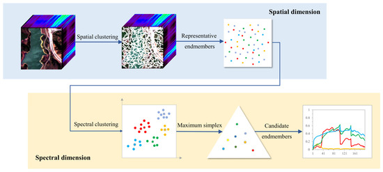
Figure 1.
The flowchart of CSVM algorithm.
2.1. Spatial Clustering
Spatial clustering can be achieved by superpixel segmentation algorithms. Here, the simple linear iterative clustering (SLIC) algorithm commonly used in two-dimensional image processing is enhanced for HSIs, as it has significant advantages in terms of calculation speed, memory efficiency and segmentation performance [28,29]. The enhancement mainly focuses on the adjustment to the clustering criterion, making it better meet the need of regional homogeneity in partitions. The details of spatial clustering are as follows.
The HSI is first divided into blocks with the size of as the initial clustering state. Take the center of each block as the cluster center. Considering that the centers located at the edge in the image may affect the clustering performance, the principal component analysis (PCA) is performed, and the projection of the image to the first principal component is chosen to calculate the gradient. The pixel with the lowest gradient in each block is regarded as new cluster center. In addition, PCA has good denoising effect, and the first principal component contains most of the information in the HSI.
Since good spatial homogeneity makes the representative endmembers more accurate, it is our primary consideration in determining the clustering principle. In some studies, clustering strategies have been developed to produce superpixels with regular sizes and shapes but poor spectral similarity, which is not suitable for us [30]. In this work, the combination of and provides constraints on spectral similarity as spectral measurement, and spatial Euclidean distance () is utilized as the spatial measurement. They are formulated as follows:
where refers to the location of a given pixel in the image,
is the center location of the partition that contains the pixel, is the length of the diagonal for the search scope used to normalize the , and are the spectra of the pixel and the cluster center respectively, and is the number of bands in the HSI.
Thereby, the spatial measurement and the spectral measurement are defined as follows:
The clustering criterion is defined as follows:
where is a weighting factor to balance and .
After initialization, spatial clustering can be iteratively conducted. In each iteration, calculate for pixels within the search scope of for each cluster center. Since a pixel may be searched for more than one time and obtain multiple , assign it to the cluster center corresponding to the smallest . Then update the cluster centers and their corresponding spectra to enter the next iteration. Pixels belonging to the same cluster center form a partition. The spatial clustering ends when all partitions no longer change. It should be noted that the designed search scope greatly reduces the computational complexity compared to global searching and makes it possible to accelerate our algorithm using parallel computation [31].
2.2. Spectral Purity Analysis
Spatial clustering obtains a set of homogeneous partitions, but the existence of mixed pixels in each partition cannot be avoided, which reduces the accuracy of representative endmembers. It is necessary to perform spectral purity analysis to choose pure pixels and remove the mixed pixels.
In the HSI, if all pixels are projected onto the same vector, endmembers will be projected to the endpoints of the vector, that is, endmembers will obtain maximum or minimum projection values. Given that each partition is considered to mainly contain one feature, pixels with higher projection values are more likely to be pure pixels. Based on that, PCA is performed on each partition, and a set of principal components decomposed by PCA is obtained denoted by . The first principal component is chosen as the projection vector, as it captures most of the information of the hyperspectral data. Then all pixels in each partition are projected on it as follows:
where is a partition containing pixels, and is a set of projection values of this partition.
To find pixels with high spectral purity, sort in descending order and obtain new vector . Choose pixels in order according to certain proportion Pt from , and take the average of the chosen pixels as a representative endmember for each partition, which alleviates the local-scope spectral variability and random noise.
2.3. Spectral Clustering
Since the wide area covered by one class, such as ocean and forest, will be segmented into several partitions due to the constraint of the search scope, representative endmembers from these partitions exhibit the same feature. The spectral clustering plays a role in merging the representative endmembers separated. On the one hand, it is of great significance to eliminate the effect of large-scope spectral variability. On the other hand, it can reduce the number of candidate endmembers, improving the computational efficiency of the subsequent processing.
The spectral clustering method is based on the k-means clustering algorithm [32]. The clustering criterion adopts a weighted spectral measurement strategy, which takes both spectra shape and distance into consideration. It is defined as follows:
where is a balance constant.
In spectral clustering, initialize cluster centers first. Then calculate between each representative endmember and the cluster centers. Each endmember is assigned to the center with the smallest . Next, update the cluster centers according to the classification results. Perform the above operations iteratively. Representative endmembers belonging to the same cluster center form a class. The spatial clustering ends when all classes no longer change. Finally, the cluster centers are regarded as candidate endmembers, which further suppresses the effect of large-scope spectral variability.
As the final endmembers will be chosen from candidate endmembers, that is, from the cluster centers, the performance of spectral clustering is particularly key, as is the determination of the two parameters involved.
2.4. Simplex Volume Maximization
The simplex composed of endmembers has the maximum volume. Based on that, the proposed method makes the final decision on endmembers.
Suppose that the set of candidate endmembers obtained by spectral clustering is . First, it is necessary to perform PCA on to reduce the dimension to and obtain a new set denoted by . represents the number of endmembers. The simplex volume is calculated as follows:
Iteratively select vectors from
and calculate the corresponding . The vectors with the largest are selected as the final endmembers. It can be formulated as follows:
3. Results and Discussion
In this section, parameter analysis is first carried out to choose the optimal value for each parameter in CSVM and improve the applicability of CSVM for future use. Then four experiments are performed on three datasets (the Samson dataset, Jasper Ridge dataset, and Cuprite dataset) to evaluate the performance of the proposed method. The comparison algorithms include VCA, SGA, AVMAX, MVSA, AMEE, ESCO, KMEE, FSPM, SENMAV, SPEW. Among them, VCA, SGA and AVMAX are convex geometry-based methods commonly used for comparison; AMEE and ESCO are typical methods that integrate spatial and spectral information; MVSA, KMEE and FSPM are noise-robust algorithms, and the result of FSPM is sent to VCA to determine the final endmembers, as it is a preprocessing module; SENMAV and SPEW combine clustering with a simplex-based algorithm, which is similar to our approach. Since hyperspectral unmixing involves endmember extraction and abundance estimation, the first two experiments aim to compare the performance of all test algorithms on endmember extraction and abundance estimation, respectively. The third experiment verifies the noise robustness of all algorithms by setting the signal-to-noise (SNR) level of the datasets to 15 dB, 20 dB, 25 dB, 30 dB, 35 dB and 40 dB. In the fourth experiment, the processing time of all methods are compared, and the acceleration possibility of the proposed method is analyzed. To ensure the reliability of the experimental results, each experiment is conducted five times and the average values are taken in this paper.
3.1. Input Data
3.1.1. Samson Dataset
Samson contains 156 bands covering the wavelength range from 401 nm to 889 nm with the spectral resolution of 3.13 nm. It has no blank channels or badly noised channels. To reduce the computational cost, the Samson dataset used in our experiment is partially cropped from the original image starting with the (252,332) pixel, which has the size of 95 × 95 and three endmembers corresponding to soil, tree, and water. The pseudo-color image and the spectral reflectance of endmembers are shown in Figure 2 [33].
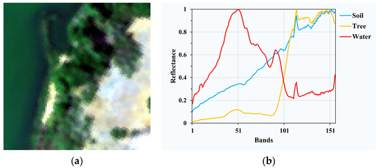
Figure 2.
(a) Pseudo-color image of Samson; (b) spectral signatures of endmembers in Samson.
3.1.2. Jasper Ridge Dataset
Jasper Ridge has 224 bands ranging from 380 nm to 2500 nm with the spectral resolution of 9.46 nm. Due to the dense water vapor and atmosphere effect, bands 1–3, 108–112, 154–166 and 220–224 are removed, and 198 bands are reserved for experiments. Additionally, a sub-image of 100 × 100 pixels starting with the (105,269) pixel from the original image is used, as shown in Figure 3. There are four endmembers in this data: road, soil, water and tree.
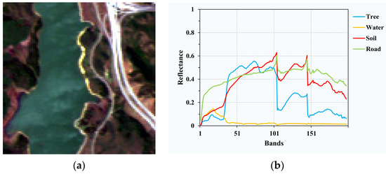
Figure 3.
(a) Pseudo-color image of Jasper Ridge; (b) spectral signatures of endmembers in Jasper Ridge.
3.1.3. Cuprite Dataset
Cuprite is one of the most widely used hyperspectral data for hyperspectral unmixing, which contains 224 bands ranging from 370 nm to 2480 nm. The noised bands (1–2 and 221–224) and the water absorption bands (104–113 and 148–167) are removed, and 188 bands are retained. A sub-image of 250 × 190 pixels is utilized in our experiments, including 14 minerals. To avoid the minor difference between the variants of the same mineral, 12 minerals are finally considered as endmembers, which are alunite, andradite, buddingtonite, dumortierite, kaolinite1, kaolinite2, muscovite, montmorillonite, nontronite, pyrope, sphene and chalcedony as shown in Figure 4.
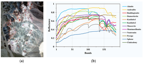
Figure 4.
(a) Pseudo-color image of Cuprite; (b) spectral signatures of endmembers in Cuprite.
3.2. Parameter Analysis
The input parameters for CSVM include , , , , and . The number of endmembers is denoted by , which can be obtained by endmember number estimation algorithms. The grid step s, the weighting factor and the proportion for representative endmember extraction will be set through the following spatial clustering analysis. The weighting factor and the number of clusters will be determined in the following spectral clustering analysis.
Indexes are first introduced to provide a quantitative assessment for the clustering performance, including , and corresponding to the following definitions.
where is the variance of HSI and is the variance of the ith partition.
where is the correlation coefficient between and the average vector in the ith partition, and is the number of pixels contained in this partition.
where is the jth singular value after singular value decomposition.
The smaller the value of Scatt and the larger the value of and , the better the clustering results.
3.2.1. Spatial Clustering Analysis
Spatial clustering involves the grid step and the weighting factor for spatial measurement . Two experiments are designed to determine the optimal values of them. To determine s, set to 0.9, and calculate , and on the input datasets clustered with from 5 to 30. The results are shown in Figure 5. To determine , set to 6, and , and are calculated on the input datasets clustered with from 0 to 1 at an interval of 0.05. The results are shown in Figure 6.
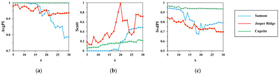
Figure 5.
The results of (a) ; (b) ; (c) with the change of .
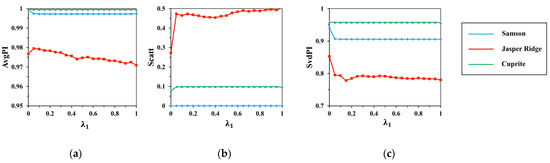
Figure 6.
The results of (a) ; (b) ; (c) with the change of .
From Figure 5, the indexes fluctuate significantly with the increase in , and from Figure 6, the indexes keep stable with the increase in . It shows that has a greater impact on the clustering performance than .
Of all the datasets, Cuprite is in sharp contrast with Samson and Jasper Ridge. The indexes on Cuprite turn out to be the most stable. Especially in Figure 5, the indexes have a relatively slight change, with rising from 5 to 30. This has relations with the spectral contrast of endmembers in datasets. As shown in Figure 4, Cuprite contains endmembers with minor difference, while endmembers in Samson and Jasper Ridge have high spectral contrast.
With the rise in , both and trend down and trends up. It can be inferred that a large will lead to high dispersion degree and low spectral correlation as each partition is expanded. However, a small will increase the computational cost. As is presented in Figure 5, the indexes keep steady as rises from 5 to 10, so the best range for is set to 5–10. In our experiments, is set to 6.
When is 0.05, the indexes have a sharp change, as the spatial measurement begins to constrain clustering. Then, the indexes tend to be stable because of the limitation of the search scope. Indexes on Samson and Cuprite have little change, but it is different on Jasper Ridge. Specifically, AvgPI and SvdPI fall steadily and Scatt rises slowly. It is away from our requirement of regional homogeneity. Hence, is set to 0.1 to keep the stability as well as good performance of spatial clustering.
Figure 7 shows the results of spatial clustering with the parameters set above. For better viewing, part of each image is enlarged and shown in the red box.
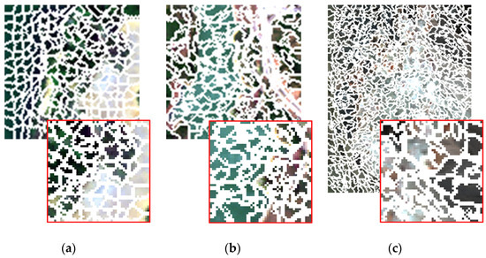
Figure 7.
The results of spatial clustering. (a) Samson; (b) Jasper Ridge; (c) Cuprite.
represents the percentage of pixels reserved from each partition for representative endmember generation. To analyze the impact of , an experiment is conducted. After completing the spatial clustering with and being 6 and 0.1, respectively, choose pixels in each partition with from 0.05 to 0.95 at an interval of 0.01, and the indexes are calculated each time. The results are shown in Figure 8.
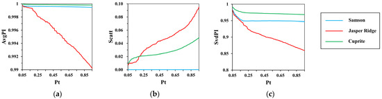
Figure 8.
The results of (a) ; (b) ; (c) with the change of .
Compared to Samson and Cuprite, indexes on Jasper Ridge have the most obvious change. It is caused by its poor spatial homogeneity. The increase in results in the decline in and and the rise in as more mixed pixels within each partition are preserved. In terms of dispersion degree and spectral correlation, the smaller the , the better the updated partitions. Considering the prevalence of spectral variability, a small cannot help dealing with it by average the reserved pixels, otherwise it brings errors. In our experiments, is set to 0.4, and the good performance will be demonstrated in subsequent experimental results.
Moreover, compared to the indexes in Figure 6, and increase to above 0.99 and 0.85, respectively, and decreases to below 0.1. It further shows the important role of spectral purity analysis on regional homogeneity.
3.2.2. Spectral Clustering Analysis
There are two parameters involved in spectral clustering: the weighting factor and the number of clusters . The experimental basis of spectral clustering analysis is the completion of spatial clustering with s of 6 and of 0.1 and representative endmember generation with of 0.4. To choose the best value for and , the following experiments are carried out. First, set to 0.4, calculate , and on the spectral clustering results with from to 10* at an interval of . The results are shown in Figure 9. Then, set to 5*, and indexes are calculated on the k-means clustering results as increases from 0 to 1 with an interval of 0.05. The results are demonstrated in Figure 10.
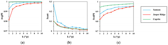
Figure 9.
The results of (a) ; (b) ; (c) with the change of .
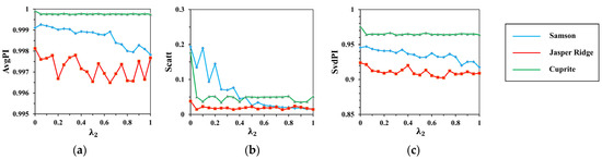
Figure 10.
The results of (a) ; (b) ; (c) with the change of .
It can be seen from the results that the response range of each index to is greater than that to , which indicates that has a greater impact on spectral clustering than . Similar to spatial clustering, indexes on Cuprite are the most stable compared to that on Samson and Jasper Ridge. This has relations with the different spectral contrast of endmembers in the datasets.
When is below 5*, and rise rapidly, and then tend to stabilize. shows a fall trend, and roughly takes of 5* as the cut-off point. That is, when the number of clusters is more than five times the number of endmembers, the spectral clustering keeps good performance with low dispersion degree and high spectral correlation within classes. At the same time, a large may lead to over-clustering, as the same feature with spectral variability will be divided into different classes. Taking all this into consideration, set to 5*. This number improves the computational efficiency of searching for the maximum simplex volume compared with other simplex-based algorithms.
With the increase in , all indicators show a falling trend. That is, the reinforcement of spectral distance constraint enhances the central tendency but weakens the spectral shape similarity. To keep low dispersion degree and good spectral correlation, the best value of is set to 0.4.
3.3. Evaluation Metrics
Metrics are used to evaluate the performance of all test algorithms in terms of endmember extraction, abundance estimation and noise robustness.
estimates the shape similarity between the spectra of the real endmember and the extracted endmember by calculating the angle of them. The smaller the value of , the more similar the two spectra.
The root mean square error () calculates the error between the real abundance vector and the estimated abundance vector for each endmember. The fully constrained least squares (FCLS) algorithm is utilized to obtain the abundance map in this work [34]. A smaller means a higher unmixing accuracy with the extracted endmembers.
3.4. Results for Endmember Extraction
In this part, the performance of all algorithms on endmember extraction is compared. According to the previous parameter analysis, , , , and are set to 6, 0.1, 0.4, 0.4 and 5* respectively. Figure 11, Figure 12 and Figure 13 give the comparison between the estimated and ground-truth endmember spectral signatures of Samson, Jasper Ridge and Cuprite, respectively. The calculation results are shown in Table 1.
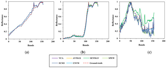
Figure 11.
Comparison between the estimated and ground-truth endmember spectral signatures on Samson. (a) Soil; (b) tree; (c) water.
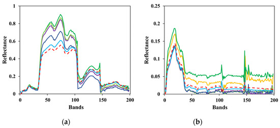
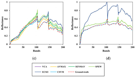
Figure 12.
Comparison between the estimated and ground-truth endmember spectral signatures on Jasper Ridge. (a) Tree; (b) water; (c) soil; (d) road.
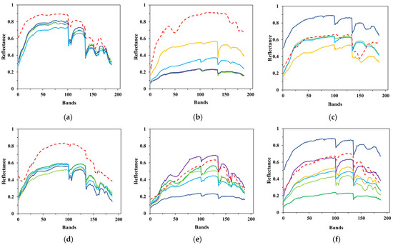
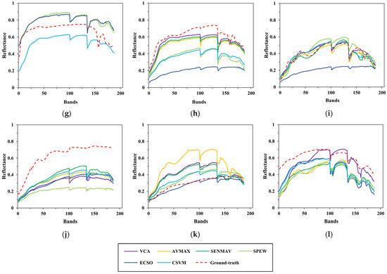
Figure 13.
Comparison between the estimated and ground-truth endmember spectral signatures on Cuprite. (a) Alunite; (b) andradite; (c) buddingtonite; (d) dumortierite; (e) kaolinite1; (f) kaolinite2; (g) muscovite; (h) montmorillonite; (i) nontronite; (j) pyrope; (k) sphene; (l) chalcedony.

Table 1.
SAD of all test algorithms on Samson, Jasper Ridge and Cuprite datasets.
To clearly show the comparison, the results of several test algorithms that perform better are drawn in the figures above, including VCA, AVMAX, SENMAV, SPEW and ECSO. From Figure 11, most algorithms can accurately extract soil and tree, but have a relatively large extraction error on water. CSVM achieves the best extraction accuracy on soil and water, as the curves almost coincide with the ground truth. Figure 12 shows the comparison for Jasper Ridge. According to the curves, all endmembers obtained by CSVM show the best consistency with ground truth in terms of shape and reflectance value. Figure 13 depicts the results for Cuprite. It is difficult to directly evaluate the algorithms through the curves since they all have difference with the ground truth in both shape and reflectance value. Therefore, quantitative analysis is necessary for further evaluation.
Table 1 shows the results of SAD. In Samson, CSVM obtains the best for Soil and Water. SGA fails to extract water, as it gets a more than 1, and KMEE fails to extract tree. CSVM provides best s on all endmembers in Jasper Ridge. SGA and KMEE are unable to extract water, and AMEE fails to extract road. All algorithms extract endmembers in Cuprite. CSVM gets the best results on dumortierite and chalcedony. CSVM does not achieve best extraction accuracy on all endmembers. For those that do not get the best , such as tree in Samson, muscovite in Cuprite and so on, CSVM obtains the results that are very close to the best values. Overall, CSVM provides the best averages for all datasets, corresponding to 0.0179, 0.0599 and 0.0873, respectively.
Compared to Cuprite, CSVM performs better on Samson and Jasper Ridge and greatly improves the extraction accuracy. The different performance on different datasets has relation to the spectral contrast of endmembers in the datasets. Cuprite has spectrally similar endmembers coupled with the effects of spectral variability, bringing difficulties to accurate extraction [35].
In conclusion, CSVM exhibits the best performance on endmember extraction, as it effectively alleviates the spectral variability. In addition, CSVM performs better for datasets with high spectral contrast of endmembers.
3.5. Results for Abundance Estimation
To evaluate the performance of all algorithms on abundance estimation, the endmembers obtained by these algorithms are adopted to generate abundance maps through the FCLS algorithm. RMSE is calculated between the estimated abundance vector and ground-truth abundance vector. The results are shown in Table 2. Because there are no ground-truth abundance maps for Cuprite, only Samson and Jasper Ridge are used in this section. It is noted that the unmixing result is an indirect verification of EEAs, as it also relies on the abundance estimation algorithm.
Table 2.
RMSE of all test algorithms on Samson and Jasper Ridge datasets.
From the results, CSVM obtains the best RMSE on soil and the best average for Samson. For Jasper Ridge, CSVM provides the best RMSE on tree, water and road and the best average. It indicates that the endmembers extracted by CSVM reduce the error of abundance estimation.
Therefore, compared with other EEAs, our method achieves better performance in hyperspectral unmixing considering endmember extraction and abundance estimation, comprehensively.
Figure 14 and Figure 15 demonstrate the comparison between estimated abundance maps using endmembers extracted by CSVM and the ground truth. As is shown in absolute error maps, CSVM obtains smaller estimation error on endmembers in Jasper Ridge than that in Samson, which means CSVM performs better on Jasper Ridge than on Samson. In addition, the results on both datasets show that the absolute error is large in areas with complex ground objects distribution, especially in the transition areas with different land cover types on both sides.
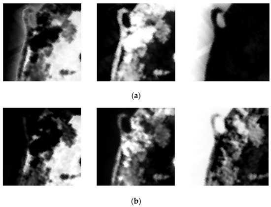
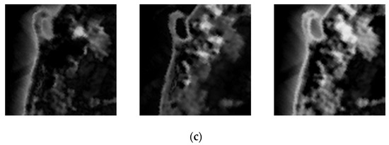
Figure 14.
From left to right are (a) the ground-truth abundance maps; (b) the estimated abundance maps; (c) absolute error maps of soil, tree and water in Samson.
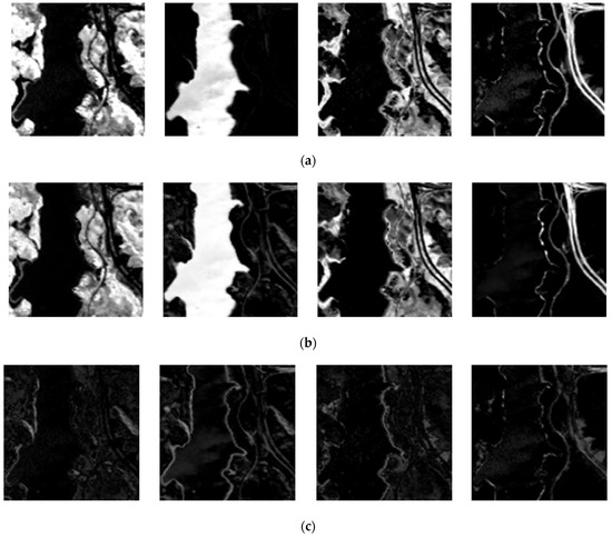
Figure 15.
From left to right are (a) the ground-truth abundance maps; (b) the estimated abundance maps; (c) absolute error maps of tree, water, soil and road in Jasper Ridge.
3.6. Results on Noisy Datasets
To verify the noise robustness of the test algorithms, set the SNR of the datasets to be 15 dB, 20 dB, 25 dB, 30 dB, 35 dB and 40 dB, then all algorithms are used to extract endmembers on the datasets. The average SAD between estimated endmembers and ground-truth endmembers are recorded in Table 3.
Table 3.
The average SAD of all test algorithms on noisy Samson, Jasper Ridge and Cuprite datasets.
It can be seen from the results that with the increase in SNR, the average s commonly decline and achieve the best results at 40 dB. It shows that noise will distort the spectra of endmembers and reduce the extraction accuracy. There are special cases in all test algorithms. Since SGA cannot extract all endmembers as previous analyzed, the results of it have a slight change with the increasing of SNR. KMEE has anti-noise ability, but its average SADs vary greatly due to the unstable endmember extraction results. FSPM exhibits strong noise robustness, especially on the Cuprite dataset. As MVSA replaces positive hard constraint on abundance with a soft constraint of hinge loss type, it also shows good robustness to noise.
In addition, when SNR is below 30 dB, the results change obviously; when SNR is above 30 dB, the results have little change. It can be inferred that when SNR is set to 30 dB and above, the datasets may reach their best quality, thus limiting the extraction accuracy. Compared to Samson and Jasper Ridge, most algorithms seem to show better anti-noise performance on Cuprite, as the average SADs on Cuprite rise slowly with the decrease in SNR. This could be resulted from its low spectral contrast of endmembers.
Overall, AMEE exhibits weak noise robustness. It has larger averages than other algorithms when SNR is at a low level. CSVM obtains best extraction accuracy for all endmembers of datasets and achieves the best anti-noise performance.
3.7. Comparison on Processing Time
All the algorithms are implemented on Matlab R2019a with an Intel Core i5-10210U CPU at 1.60 GHz. The processing time of each test algorithm is shown in Table 4.
Table 4.
CPU processing time of all test algorithms on Samson, Jasper Ridge and Cuprite datasets (in seconds).
It is noted that ECSO is the most time-consuming algorithm, which requires a lot of computations. VCA is the most efficient method, as it takes a short time and provides high accuracy on endmember extraction. CSVM consumes a certain time due to the spatial clustering operation. This issue can be solved by the graphics processing units (GPU) parallel platform, as it shows superior performance in floating-point operations and programming. The superpixel segmentation provides possibility for parallel acceleration of CSVM.
4. Conclusions
In this paper, an endmember extraction method based on quadratic clustering is proposed to better handle spectral variability. CVSM first adopts SLIC-based spatial clustering to segment HSI into homogeneous partitions, and the average of pure pixels obtained by spectral purity analysis in each partition is taken as representative endmember, which reduces the effect of local-scope spectral variability. Then CVSM performs spectral clustering to merge spectrally related representative endmembers to further alleviate large-scope spectral variability, and the final endmembers are determined by simplex with maximum volume. CSVM is implemented from spatial and spectral dimension, which takes full of spatial and spectral information and effectively eliminates the effect of spectral variability.
Experiments are conducted to evaluate the performance of CSVM in terms of endmember extraction, abundance estimation, noise robustness and processing time. Through parameter analysis, the optimal parameters are first set for our experiments and future use. From the experimental results, the following can be concluded: (1) CSVM greatly improves the extraction accuracy by reducing the effect of spectral variability and performs better on datasets with high spectral contrast between endmembers; (2) CSVM provides better performance on abundance estimation with FCLS abundance estimation algorithm; (3) because of the average operations after clustering, CSVM also shows strong noise robustness; and (4) clustering makes CSVM consume lots of time, and it is one of our future research topics to further accelerate our method.
Author Contributions
Conceptualization, X.Z.; methodology, X.Z.; software, X.Z.; validation, X.Z.; formal analysis, X.Z.; investigation, X.Z.; resources, X.Z.; data curation, X.Z.; writing—original draft preparation, X.Z.; writing—review and editing, T.X.; visualization, T.X.; supervision, Y.W.; project administration, Y.W. All authors have read and agreed to the published version of the manuscript.
Funding
This research received no external funding.
Institutional Review Board Statement
Not applicable.
Informed Consent Statement
Not applicable.
Data Availability Statement
Not applicable.
Conflicts of Interest
The authors declare no conflict of interest.
References
- Bioucas-Dias, J.M.; Plaza, A.; Camps-Valls, G. Hyperspectral Remote Sensing Data Analysis and Future Challenges. IEEE Geosci. Remote Sens. Mag. 2013, 1, 6–36. [Google Scholar] [CrossRef] [Green Version]
- Li, R.X. Improving Hyperspectral Subpixel Target Detection Using Hybrid Detection Space. J. Appl. Remote Sens. 2018, 12, 1. [Google Scholar] [CrossRef]
- Song, X.R.; Zou, L.; Wu, L.D. Detection of Subpixel Targets on Hyperspectral Remote Sensing Imagery Based on Background Endmember Extraction. IEEE Trans. Geosci. Remote Sens. 2021, 59, 2365–2377. [Google Scholar] [CrossRef]
- Zhang, Y.; Huang, X.D.; Hao, X.H. Fractional Snow-cover Mapping Using an Improved Endmember Extraction Algorithm. J. Appl. Remote Sens. 2014, 8, 84691. [Google Scholar] [CrossRef]
- Tao, X.W.; Cui, T.W.; Ren, P. Cofactor-Based Efficient Endmember Extraction for Green Algae Area Estimation. IEEE Geosci. Remote Sens. Lett. 2019, 16, 849–853. [Google Scholar] [CrossRef]
- Hasanlou, M.; Seydi, S.T.; Shah-Hosseini, R. A Sub-Pixel Multiple Change Detection Approach for Hyperspectral Imagery. Can. J. Remote Sens. 2018, 44, 601–615. [Google Scholar] [CrossRef]
- Seydi, S.T.; Shah-Hosseini, R.; Hasanlou, M. New Framework for Hyperspectral Change Detection Based on Multi-Level Spectral Unmixing. Appl. Geomat. 2021, 13, 763–780. [Google Scholar] [CrossRef]
- Wei, J.J.; Wang, X.F. An Overview on Linear Unmixing of Hyperspectral Data. Math. Probl. Eng. 2020, 2020, 1–12. [Google Scholar] [CrossRef]
- Bioucas-Dias, J.M.; Plaza, A.; Dobigeon, N. Hyperspectral Unmixing Overview: Geometrical, Statistical, and Sparse Regression-based Approaches. IEEE J. Sel. Top. Appl. Earth Obs. Remote Sens. 2012, 5, 354–379. [Google Scholar] [CrossRef] [Green Version]
- Chang, C.I.; Wen, C.H.; Wu, C.C. Relationship Exploration among PPI, ATGP and VCA via Theoretical Analysis. Int. J. Comput. Sci. Eng. 2013, 8, 361–367. [Google Scholar] [CrossRef]
- Nascimento, J.; Dias, J. Vertex Component Analysis: A Fast Algorithm to Unmix Hyperspectral Data. IEEE Trans. Geosci. Remote Sens. 2005, 43, 898–910. [Google Scholar] [CrossRef] [Green Version]
- Winter, M.E. N-FINDR: An Algorithm for Fast Autonomous Spectral Endmember Determination in Hyperspectral Data. In Proceedings of the SPIE’s International Symposium on Optical Science, Engineering, and Instrumentation, Denver, CO, USA, 18–23 July 1999. [Google Scholar]
- Chang, C.; Wu, C.C. A New Growing Method for Simplex-Based Endmember Extraction Algorithm. IEEE Trans. Geosci. Remote Sens. 2006, 44, 2804–2819. [Google Scholar] [CrossRef]
- Chan, T.H.; Ma, W.K. A Simplex Volume Maximization Framework for Hyperspectral Endmember Extraction. IEEE Trans. Geosci. Remote Sens. 2011, 49, 4177–4193. [Google Scholar] [CrossRef]
- Li, J.; Bioucas-Dias, J.M. Minimum Volume Simplex Analysis: A Fast Algorithm to Unmix Hyperspectral Data. In Proceedings of the 2008 IEEE International Geoscience and Remote Sensing Symposium, IGARSS 2008, Boston, MA, USA, 7–11 July 2008. [Google Scholar]
- Shen, X.F.; Bao, W.X. Subspace-Based Preprocessing Module for Fast Hyperspectral Endmember Selection. IEEE J. Sel. Top. Appl. Earth Obs. Remote Sens. 2021, 14, 3386–3402. [Google Scholar] [CrossRef]
- Miao, L.; Qi, H. Endmember Extraction from Highly Mixed Data Using Minimum Volume Constrained Nonnegative Matrix Factorization. IEEE Trans. Geosci. Remote Sens. 2007, 45, 765–777. [Google Scholar] [CrossRef]
- Qian, Y.; Jia, S.; Zhou, J. Hyperspectral Unmixing Via L1/2 Sparsity-Constrained Nonnegative Matrix Factorization. IEEE Trans. Geosci. Remote Sens. 2011, 49, 4282–4297. [Google Scholar] [CrossRef] [Green Version]
- He, W.; Zhang, H.Y.; Zhang, L.P. Sparsity-Regularized Robust Non-negative Matrix Factorization for Hyperspectral Unmixing. IEEE J. Sel. Top. Appl. Earth Obs. Remote Sens. 2016, 9, 4267–4279. [Google Scholar] [CrossRef]
- Plaza, A.; Martinez, P. Spatial/Spectral Endmember Extraction by Multidimensional Morphological Operations. Geosci. Remote Sens. 2002, 40, 2025–2041. [Google Scholar] [CrossRef] [Green Version]
- Shah, D.; Zaveri, T. Entropy-Based Convex Set Optimization for Spatial–Spectral Endmember Extraction from Hyperspectral Images. IEEE J. Sel. Top. Appl. Earth Obs. Remote Sens. 2020, 13, 4200–4213. [Google Scholar] [CrossRef]
- Kowkabi, F.; Ghassemian, H. Enhancing Hyperspectral Endmember Extraction Using Clustering and Oversegmentation-Based Preprocessing. IEEE J. Sel. Top. Appl. Earth Obs. Remote Sens. 2016, 9, 2400–2413. [Google Scholar] [CrossRef]
- Xu, X.; Li, J. Regional Clustering-Based Spatial Preprocessing for Hyperspectral Unmixing. Remote Sens. Environ. 2018, 204, 333–346. [Google Scholar] [CrossRef]
- Shen, X.F.; Bao, W.X. Spatial-Spectral Hyperspectral Endmember Extraction Using a Spatial Energy Prior Constrained Maximum Simplex Volume Approach. IEEE J. Sel. Top. Appl. Earth Obs. Remote Sens. 2020, 13, 1347–1361. [Google Scholar] [CrossRef]
- Song, M.P.; Li, Y. Spatial Potential Energy Weighted Maximum Simplex Algorithm for Hyperspectral Endmember Extraction. Remote Sens. 2022, 14, 1192. [Google Scholar] [CrossRef]
- Shah, D.; Zaveri, T. Convex Geometry and K-medoids Based Noise-Robust Endmember Extraction Algorithm. J. Appl. Remote Sens. 2020, 14, 34521. [Google Scholar] [CrossRef]
- Mei, S.H.; He, M.Y. Spatial Purity Based Endmember Extraction for Spectral Mixture Analysis. Geosci. Remote Sens. 2010, 48, 3434–3445. [Google Scholar] [CrossRef]
- Achanta, R.; Shaji, A. SLIC Superpixels Compared to State-of-the-Art Superpixel Methods. IEEE Trans. Pattern Anal. Mach. Intell. 2012, 34, 2274–2282. [Google Scholar] [CrossRef] [Green Version]
- Shen, X.F.; Bao, W.X. Superpixel-Guided Preprocessing Algorithm for Accelerating Hyperspectral Endmember Extraction Based on Spatial–Spectral Analysis. J. Appl. Remote Sens. 2021, 15, 26514. [Google Scholar] [CrossRef]
- Du, Y.Z.; Chang, C. New Hyperspectral Discrimination Measure for Spectral Characterization. Opt. Eng. 2004, 43, 1777. [Google Scholar]
- Plaza, A.; Martin, G.; Plaza, J. Recent Developments in Endmember Extraction and Spectral Unmixing. In Optical Remote Sensing; Prasad, S., Bruce, L., Eds.; Springer: Berlin/Heidelberg, Germany, 2011; Volume 3, pp. 235–267. [Google Scholar]
- Hartigan, J.A.; Wong, M.A. Algorithm AS 136: A K-Means Clustering Algorithm. J. R. Stat. Soc. Ser. 1979, 28, 100–108. [Google Scholar] [CrossRef]
- Ahmed, A.M.; Duran, O. Hybrid Spectral Unmixing: Using Artifificial Neural Networks for Linear/Non-Linear Switching. Remote Sens. 2017, 9, 775. [Google Scholar] [CrossRef] [Green Version]
- Heinz, D.C.; Chang, C.I. Fully Constrained Least Squares Linear Spectral Mixture Analysis Method for Material Quantification in Hyperspectral Imagery. IEEE Trans. Geosci. Remote Sens. 2001, 39, 529–545. [Google Scholar] [CrossRef] [Green Version]
- Rogge, D.M.; Rivard, B. Integration of Spatial–Spectral Information for the Improved Extraction of Endmembers. Remote Sens. Environ. 2007, 110, 287–303. [Google Scholar] [CrossRef]
Publisher’s Note: MDPI stays neutral with regard to jurisdictional claims in published maps and institutional affiliations. |
© 2022 by the authors. Licensee MDPI, Basel, Switzerland. This article is an open access article distributed under the terms and conditions of the Creative Commons Attribution (CC BY) license (https://creativecommons.org/licenses/by/4.0/).