A Grant-Free Random Access Process for Low-End Distribution System Using Deep Neural Network

Abstract

With the rising number of Internet of Things (IoT) devices joining the communication network, data exchange is increased tremendously resulting in network congestion. This paper deals with the optimal transmission of IoT devices to maximize the chances of success in random access procedures. With every machine trying to use the network for the transfer of data, IoT devices pose serious challenges to the already deployed infrastructure network. With a huge number of IoT devices and fixed limited resources, the existing handshaking-based random access process is not effective. To address this research gap, we propose a grant-free procedure while considering orthogonal transmission and devise a strategy to minimize collisions and idle events and maximize success. We use deep neural networks (DNN) that take channel conditions as an input to predict the device’s transmission for a successful maximization. In order to evaluate the performance of our proposed algorithm, we calculated the average delay with respect to channel coefficient and arrival rate in addition to the number of successes against the channel coefficient. Simulation results show that the proposed algorithm performs well and conforms with the claim of a successful maximization.

1. Introduction

The Internet of things (IoT) is shaping a world in which not only humans but also machines use the network to exchange data. In every field of life, the devices with which humans interact are becoming smarter [1,2]. Being a smarter device means that based on the available data, the device is able to perform the tasks independently and smartly. For example, in smart grids, using data, the loads are operated in such a way that they get energy from renewable resources, and the batteries are charged such that the peak hours are avoided [3,4]. In a smart e-health system, based on the input of the patient and available data, the device decides whether to advise the patient locally or to refer him/her to a physician [5,6]. The autonomous car decides to take the route with minimum traffic based on the available data. In short, in every aspect of life, it is inevitable to interact with smart devices using data to make decisions, which makes life easier and hassle-free [7,8]. Similarly the IoT finds applications in agriculture to combat plants’ health issues and improving yield [9,10]. The smart devices exchange data with other peer devices or with the servers on the network to make their decisions.

The IoT devices that are using data are increasing at a rapid pace. According to [11], the expected number of connected IoT devices is approximately 13.8 billion units in 2021; however, it is projected to jump to 30.9 billion in 2025. After 2010, IoT devices have increased exponentially whereas the number of non-IoT devices has been almost constant. The comparison of IoT vs. non-IoT connections over the years is represented in Figure 1 where dark blue color represents non-IoT devices and light blue color represents IoT devices. It can be seen that the sharp rise in IoT devices is in the last decade, which incidentally is also the rise of the long-term evolution/long-term-evolution-advanced (LTE/LTE-A) standards. IoT devices require a network that can be used to transfer data between the devices or between devices and a server. Before the advent of LTE/LTE-A technology, the data services of the infrastructure networks were not adequate because of a lesser data rate. With LTE/LTE-A technology, the data pipe has also widened and the data rate has also increased [12,13]. This allows IoT devices to use infrastructure networks such as LTE/LTE-A networks to exchange data.

Prior to fourth generation (4G) networks, i.e., LTE/LTE-A, the infrastructure network (2G/3G) was human-centered such that both voice and data traffic were assumed to be human-centric. With the rise of the data rate in 4G networks, both humans and machines were considered for the traffic. With the popularity of the IoT and the devices outnumbering humans, the tendency has shifted to machine-centric traffic. This can be seen in the recommendations by International Telecommunication Union (ITU) for 5G [14,15]. We can see that the requirements for connection density, mobility, data rate, etc., have increased and the latency has decreased. The connection density and the latency of IoT devices specifically have values of 10⁶/km² and 1 ms (end-to-end), respectively. Grant-free transmission in the random access process of 5G technology and beyond is a process in which the devices transmit without the handshaking process described in the next section. This grant-free transmission reduces access delay for the devices.

Apart from the increase in data rate, machine/deep learning has been of massive help in smart decision-making IoT devices. As already mentioned, the devices exchange data, and based on the available data they make decisions, but with the help of techniques such as a machine or deep learning. Deep learning has been widely used in IoT applications in recent years [16,17,18,19]. IoT systems require different analytic approaches compared to traditional machine learning techniques, which should be in line with the hierarchical structure of data generation and management [20]. The IoT and deep learning for big data go hand in hand because the IoT is the source of data generation, and deep learning uses the data to improve the performance of the IoT [21,22,23]. With grant-free transmission and deep learning, a random access process can be developed which gives lesser access delay, and we deal with this problem in this work.

The contributions of our work are as follows:

• A grant-free transmission model is considered, which reduces access delay compared to conventional random access process.
• A naive Bayesian technique is used to train DNN model to predict idle, success, or collision event.
• The prediction is used to select the preamble/channel such that the probability of success is maximum, thus increasing the throughput of the system.

The rest of the paper is organized as follows: Related works is given in Section 2. The system model and the algorithm are explained in Section 3 and Section 4, while the discussion on the optimal T (threshold) is given in Section 5. The use of deep learning is explained in Section 6, the simulation results are given in Section 7, and then the paper is concluded in Section 8.

2. Related Work

As mentioned in the previous section, IoT devices can be large in numbers, which creates a serious challenge for managing the service with limited resources. After the registration of the device to the network, the provision of resources to the device is the responsibility of the eNodeB. The eNodeB schedules the transmission of the device such that the transmission is guaranteed albeit with some delay [24]. However, before the association with the network, getting connected to the network is a random process. So the access of a device is of two types, random and scheduled. Generally, more resources are allocated for the scheduled access than the random access. When the number of devices is large, the resources for random access may prove insufficient, resulting in congestion. The delay in random access becomes important since it affects the overall efficiency of the network. Moreover, if a device cannot complete the random access process successfully, it cannot have service from the network. Hence with IoT devices, the random access process becomes extremely important, and it is imperative that the devices experience less delay in this process [25,26].

In LTE/LTE-A networks, random access is a four-step handshake process between the device and eNodeB [27,28]. In the first step, the device chooses a preamble that was broadcast by eNodeB and transmits it to eNodeB. In the second step, the eNodeB responds with the random access response (RAR) message. In the third step, the device sends a connection request message to the eNodeB, and in the fourth and last step, the eNodeB sends a contention resolution to the eNodeB. 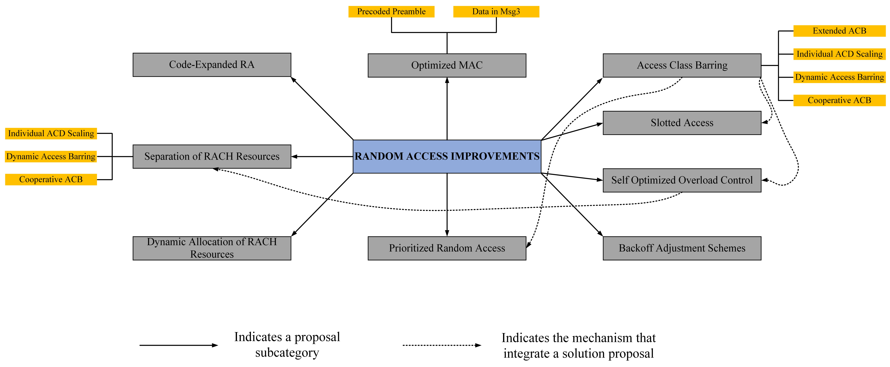The details of the random access process in LTE/LTE-A networks can be found in [29,30]. For a device to have a successful random access process, this four-step handshake process needs to be completed successfully. The problem occurs when more than one of the devices select the same preamble, which leads to the collision and the failure of the random access process of the devices involved. Therefore, controlling congestion in the random access process means minimizing the number of collisions and increasing the successful transmission. There has been a lot of work in the literature on how to control the congestion in the random access process. The techniques are discussed in [31], and in pictorial form, they are given in Figure 2.

Of all the techniques mentioned in Figure 2, access class barring (ACB) [32,33] and extended access barring (EAB) [34] have been accepted by the third-generation partnership project (3GPP) as potential solutions to overcome congestion [35]. In EAB, each device is assigned a class number ranging from zero to nine. Only one class is allowed to transmit while the other classes are barred from the transmission. The eNodeB broadcasts a bitmap consisting of 10 bits with all bits zero except the one which is allowed to transmit and it has a value of one. Each device is also assigned a paging frame (PF) and paging occasion (PO). Each device wakes up at its PO within its PF and checks whether its class is allowed to transmit or not. If allowed, it transmits, otherwise it waits for the next PF and PO. The chances of collision in EAB are less but the delay is larger due to a large idle time. The devices have to wait for longer periods of time for successful transmission. In ACB, the eNodeB broadcasts an ACB factor (a transmission probability). Each device generates a random number and if this random number is less than the ACB factor, the device transmits, otherwise it is barred from the transmission and it waits for the next chance. In ACB, the idle time is less, but the collisions are more, and the delay in ACB is less than that of EAB. In ACB, the ACB factor is of prime importance and needs to be optimal to have a maximum success probability. In [29], it was derived that the optimal transmission probability can be written as:

$$p_{opt}=min\left(1,\frac{M}{n}\right),$$

(1)

where M is the number of preambles (or channels), and n is the number of devices.

The focus is now shifting to the grant-free transmission, i.e., when $p_{opt}=1$. With $p_{opt}<1$, there can be some devices that are barred from the transmission and hence experience delay. If $p_{opt}=1$, all the devices transmit, reducing the delay. The four-step handshake process also induces a delay. With the grant-free procedure, each device can transmit at any time of its choice. It does not need to take permission from the eNodeB for transmission. However, with the grant-free transmission, there comes a challenge. If all the devices transmit simultaneously, collisions can take place. If the number of resources is larger than the number of devices, the grant-free process outperforms the conventional handshake-based random access process. However, if number of devices is larger than the number of resources, which is generally the case, collisions can take place and the performance will be worse than the conventional random access process. Therefore, in order to make the grant-free process work, a sophisticated technique or algorithm is required such that the collisions are minimized and success is maximized. In [36], the authors studied grant-free transmission, where the resource pool was increased virtually, such as in pattern division multiple access (PDMA) [37]. In [38], the authors used multiple antennas to increase the success probability of the preambles; however, the model used in our work is simpler as it only considers a single antenna. In [39], the authors used collision reduction to solve the problem of congestion in grant-free random access process in a massive MIMO scenario. Again, the receiver complexity was the issue, which is nonexistent in our scenario. The authors in [40] used sparsity and then used signal processing techniques at the receiver to decode which transmitter had transmitted on the channel; however, it increased the receiver complexity, while the algorithm in our work requires a simple receiver. In this way, there are enough resources for the devices to choose separate channels and hence collisions can be reduced.

So far, we have discussed grant-based random access, grant-free random access, and the techniques that are used to implement the grant-free transmission. Most of the techniques used signal processing techniques or nonorthogonal transmission to resolve the problem of collision. We did not find any work where grant-free transmission was obtained without complex signal processing at the receiver and orthogonal transmission. In this paper, we take this challenge and propose an algorithm for grant-free transmission without receiver complexity and orthogonal transmission with the objective to minimize collisions. We use deep learning techniques to realize our algorithm. In the first step, our deep learning model is trained based on the scenarios of idle, success, and collisions. Then, the deep learning model is used to predict the run time and which device needs to transmit such that there is a maximum chance of success and a minimum chance of collision.

3. System Model

As already mentioned above, for the system model, we consider a grant-free transmission. Let us denote by M the total number of preambles or channels, and D the total number of IoT devices trying to transmit to the network. Unlike in [36], in which the resource pool was increased to incorporate a large number of IoT devices, we take a slightly different approach by introducing stations N. 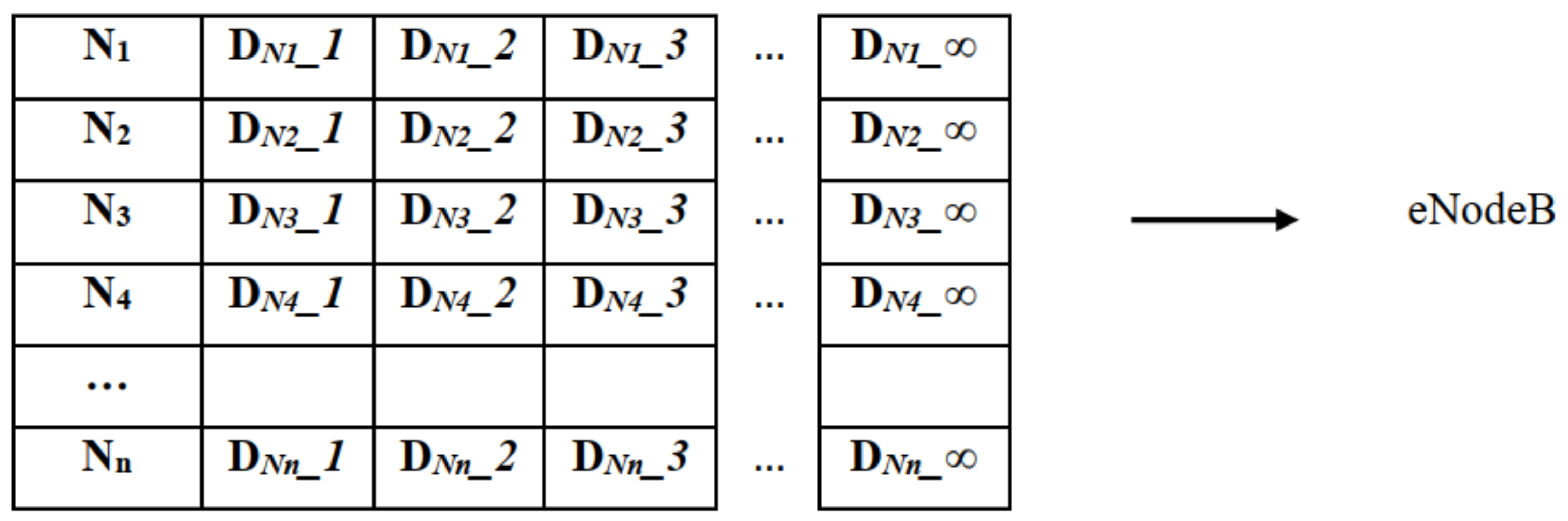The IoT devices, instead of transmitting directly to the eNodeB, transmit to any of the N stations randomly. If there is no queue in the station, the device directly transmits to the eNodeB, otherwise, it waits until the queue ends. Each station has an infinite queue to incorporate a large number of IoT devices. The IoT device emulates a unit buffer queue or a node, and it has one packet. Any real time IoT device can be considered, especially the devices that send data on a consistent basis. The devices may have the following properties: a unit buffered queue, small size of the transmitted data, and a Poisson based distribution. The devices can be considered as operating from batteries because of the small size of the packet and sporadic transmission. The device leaves the system as soon as it achieves success and competes for the channel again after obtaining a packet. The pictorial representation of the system model is given in Figure 3.

We see that in Figure 3, the rows represent different stations and the columns in each row represent the devices. The number of stations is limited while the number of devices that transmits via stations is infinite. $D_{N1\_1}$ represents the first device in station $N_1$ and $D_{N3\_2}$ represents the second device in station 3, etc. The devices arrive in the system based on a Poisson arrival process, with $\lambda$ being the arrival rate. Each device has only one packet, and as soon as it gets successful, it leaves the system and tries again when it has a packet. So, in our scenario, devices and packets are the same things and may be used interchangeably throughout the text.

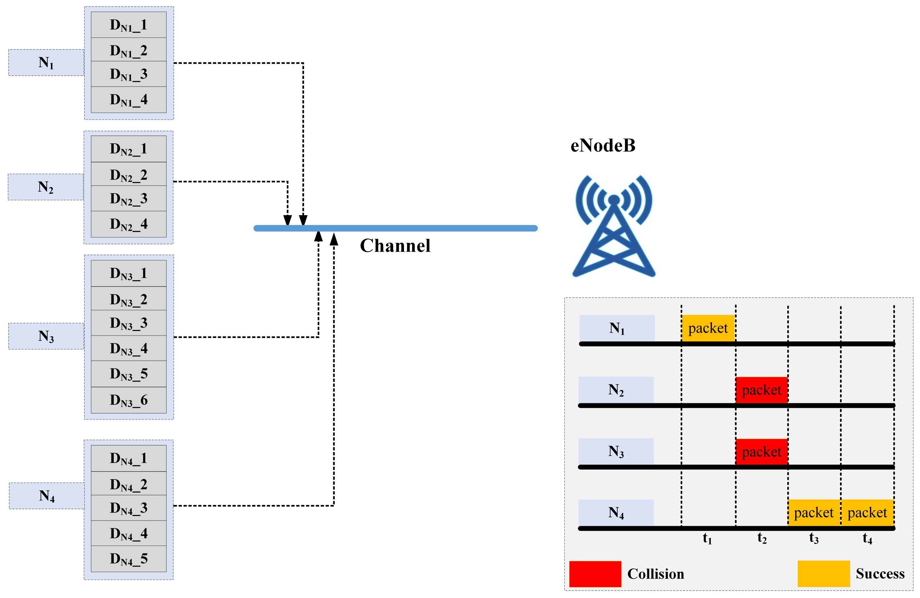
When the device arrives at the station, it checks whether there is a queue ahead of it or not. If there is no queue, which means there is only one device in that station, the device immediately transmits, otherwise, it enters the queue. If there are multiple devices in a queue, the device with maximum waiting time transmits, i.e., it follows the first-in-first-out (FIFO) rule.

At the start of each time slot, the station which has the device transmits the packet to the eNodeB. If only one station transmits and others remain idle, the event is a success, whereas if more than one of the stations have a packet and they transmit, it results in a collision. If queues of all the stations are empty, the event is idle. This is depicted in Figure 4.

Since the handshake process and ACB are not used in grant-free transmission, it needs a sophisticated algorithm to keep the number of collisions to a minimum and the number of successes to a maximum. The proposed algorithm is able to predict which station should transmit to have a minimum number of collisions and maximum number of successes. The algorithm is explained in the next section.

4. The Algorithm

As already mentioned, the algorithm tells which station needs to transmit. To achieve this feat, we divide our task into two parts. In the first part, we use our proposed algorithm, Algorithm 1, to train the DNN model. In the second part, the trained DNN is used to predict the transmission of the desired station. Here, we first explain the algorithm, and then later, the DNN model is also explained. The main parameter on which the algorithm depends is the channel coefficient represented by $CC\in (0,1)$. The other secondary but equally important parameters are the channel outcome represented by $CO$ and the previous three transmissions, represented by $PT$. $CO$ is the outcome of the channel such as idle, success, and collision, represented by 0, 1, and 2, respectively. $PT$ is the previous three transmissions of each station, whether the previous three transmissions have collided or not. Let us denote by T, the threshold used to make decisions based on $CC$.

For each device, the $CC$ is checked to see whether it is above the threshold T or not. $CC$ is the representation of the channel between the station and the eNodeB. A higher value of $CC$ represents a good channel whereas a bad channel has a smaller value of $CC$. If no device has $CC>T$, this means that no device in any station is eligible for the transmission, and the outcome of the channel is considered to be idle. This condition happens in lightly loaded traffic, where the arrival of the devices at stations is very sporadic. If only one device meets the condition $CC>T$, then it is a success, because it is the only device that is eligible for transmission. The other devices simply refrain from transmitting as they are not eligible. However, if more than one device fulfills the condition $CC>T$, then success cannot be guaranteed, and other conditions also need to be checked. At this point, the other parameter with the condition $PT\ne 3$ is checked. If only one device fulfills this condition, then it is a success. The other devices that fulfill the $CC>T$ condition but could not fulfill the $PT\ne 3$ condition are prevented from transmitting, resulting in success. It is possible that more than one device fulfills both the above-mentioned conditions, and then comes the third condition $CO=1$. Similarly, if only one device has $CO=1$ then it is a success, otherwise, it is a collision. So, by incorporating multiple conditions, the probability of success is increased. It becomes extremely useful especially in lightly loaded conditions where the arrival of devices is not in bursts. Therefore, we see that the algorithm largely depends on T and associated conditions. A careful choice of T may result in a better performance of the system which is discussed in the next section.

Algorithm 1 Algorithm to train the DNN

1: Initialize N, M, $CO=0$, $PT=0$ 2: For each device check the channel coefficient $CC>T$ 3: if no device has $CC>T$ then 4:      the event is idle 5: else if one device has $CC>T$ then 6:      the event is a success 7: else if more than one device has $CC>T$ then 8:      check for a value of $PT\ne 3$ 9:      if one device has $PT\ne 3$ then 10:         the event is a success 11:    else if then 12:         check for the value of $CO=1$ 13:         if one device has $CO=1$ then 14:            the event is a success 15:         else if then 16:            the event is collision 17:         end if 18:      end if 19: end if 20: Update $CO$ and $PT$

5. Optimal T

The threshold T plays an important role in enhancing the performance of the system by affecting performance metrics such as the delay and success rate. T should not be constant across all arrival rates as it may badly affect the performance of the system on some arrival rates. If the arrival rate is low and T is also low, it means that the traffic is sparse and may not qualify for transmission due to the low value of T. The result is more idle traffic. On the other hand, if the arrival rate is high and T is also high, the large number of devices may qualify for transmission, and hence collisions will take place. Therefore, the value of T should vary with the arrival rates and should be optimal such that the idle traffic and collisions are minimized and success is maximized. Hence, we face another subproblem of constrained optimization.

$$\begin{array}{cc}\hfill \underset{T,PT,CO}{max}\hspace{1em}& Success\hfill \end{array}$$

(2)

To find out the optimal T, the number of successes is calculated for a value of the arrival rate with changing values of T, $PT$, and $CO$. Then, the value of T and other parameters are chosen that give a maximum value to the number of successes. Then, the optimal value of T is used afterwards.

6. The Use of Deep Learning

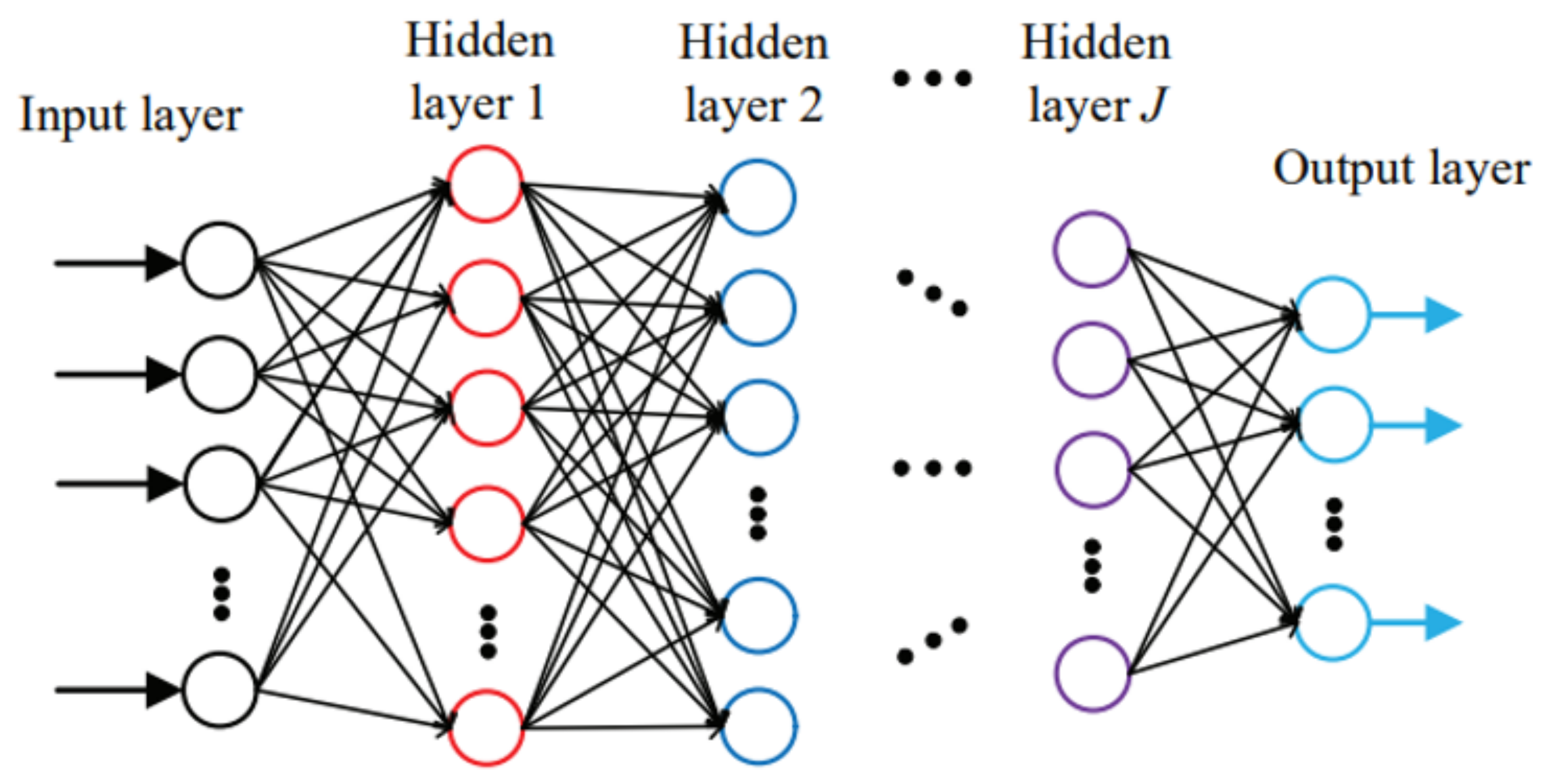
To solve our problem, we considered a four-layer feed-forward neural network. Unlike ML, where the optimal solution can be found by using one or two layers of data transformation to learn the output representation, deep learning provides a multilayer approach to learning the data representations typically performed with a multilayer neural network. There are different ways to model in deep learning and the most common and simplest of them is a feed-forward neural network also known as multilevel perceptron. The pictorial representation of the feed-forward neural network is shown in Figure 5.

As we can see from Figure 5, there are four entities in neural networks, namely, the input layers, hidden layers, output layers, and weights. Normally, a classifier maps an input x to the output y via a $y=f(x\ast )$ function, whereas, in deep learning, the feed-forward network defines a new mapping $y=f(x;\theta )$ and then learns the value of the parameter $\theta$ that can make the best approximation of the function. The models are called feed-forward because the information is evaluated using x through the function f while using the computations in the intermediate layers, and based on these values, the output y is calculated. There are no feedback connections among the layers as opposed to the backpropagation model where we can also go in the backward direction.

Normally, the output of a neuron is 0 or 1, but in this model, since weighted sums are involved, the output of a neuron is no longer 0 or 1 but a real number. This calls for a decision methodology based on some threshold, which is called the activation function.

We used a sigmoid as an activation function where the output is +1 or 0 for the inputs above or below the threshold, respectively, if the selected threshold is taken to be 0.5. The sigmoid function, which has a mathematical representation of $F=\frac{1}{1+e^{-}x}$, is represented as in Figure 6:

7. Simulation Results

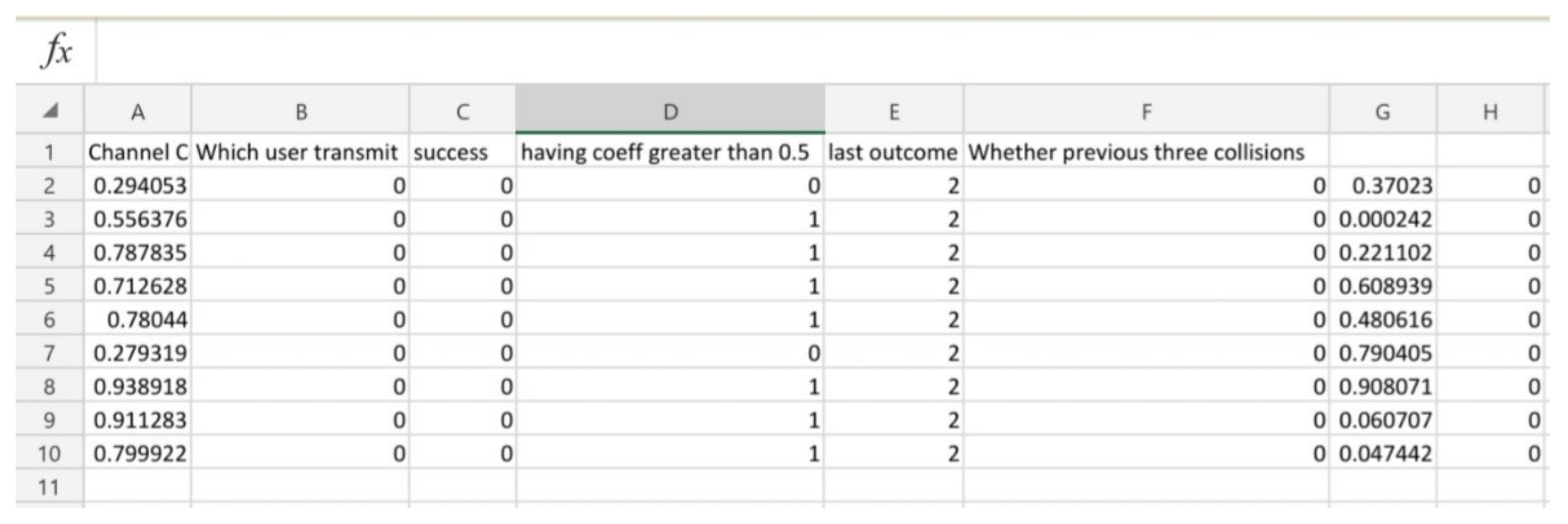
Before discussing the simulation results, let us explain the feature extraction and training process of the DNN. Figure 7 shows a screenshot of the features extracted. We see that there are 10 rows with each row representing a station and within each station, there is an infinite number of devices that are represented by columns. For each device, six features are extracted and stored. The first six columns of the first row represent the features of the first device in the first station. The columns from 7 to 12 in the first row represent features of the second devices of the first station and so on. The features extracted are as follows:

• The channel coefficient;
• The transmitting device;
• The successful device;
• The devices that have coefficients greater than the threshold;
• The last outcome of the channel;
• An indicator whether the previous three transmissions of the device are collisions.

Figure 7. Extracted features to train the DNN.

Figure 7. Extracted features to train the DNN.

A channel coefficient is a random number between zero and one drawn from a normal distribution. The second feature tells us whether the device transmits or remains idle. If its value is one, it means that the device has transmitted whereas zero represents an idle scenario. The third feature tells us which device among all is successful. Since there is only one channel, only one device can be successful, in which case this feature’s value is one, otherwise, it is zero. The fourth feature is a flag that has a value of one when the device has a channel coefficient greater than the threshold. If the value of the channel coefficient is less than the threshold, its value is zero. The last outcome of the channel means whether the previous outcome of the channel was a success, a collision, or an idle event. It is an important parameter as it tells us whether there is a large number of devices attempting transmissions or not. The last feature is related to the outcome of individual devices, whether successful, idle or a collision. This feature is different from the previous one, as in the previous feature the outcome of the channel was discussed while in this feature, the outcome of the individual device is considered.

With all the features in hand, we needed to accumulate success scenarios such that the features vividly point to the successful device. Once it was done, then the data were fed to the DNN, which extracted the features depending on the success scenario. Then, the fully trained DNN was able to tell us in real-time which device needed to transmit to get maximum success and minimum collisions.

Let us discuss the simulation results after we apply Algorithm 1 to our system model. The number of stations for the simulation was taken to be four and an infinite number of devices were allowed to arrive and access the channel. In case of collision or idle event for a device, which can result from the channel being busy, the devices could queue up at the stations. The stations randomly accessed the channel based on a slotted ALOHA protocol; however, the transmission was governed by Algorithm 1. The arrival distribution was assumed to be Poisson with the arrival rate changing for each set of simulations. The output parameters considered were the average access delay, the number of successes, and the number of collisions. The idle, success, and collision events were recorded to form a dataset that served as input for training the DNN. The DNN was eventually used in real-time to predict which device needed to transmit to maximize success and minimize access delay.

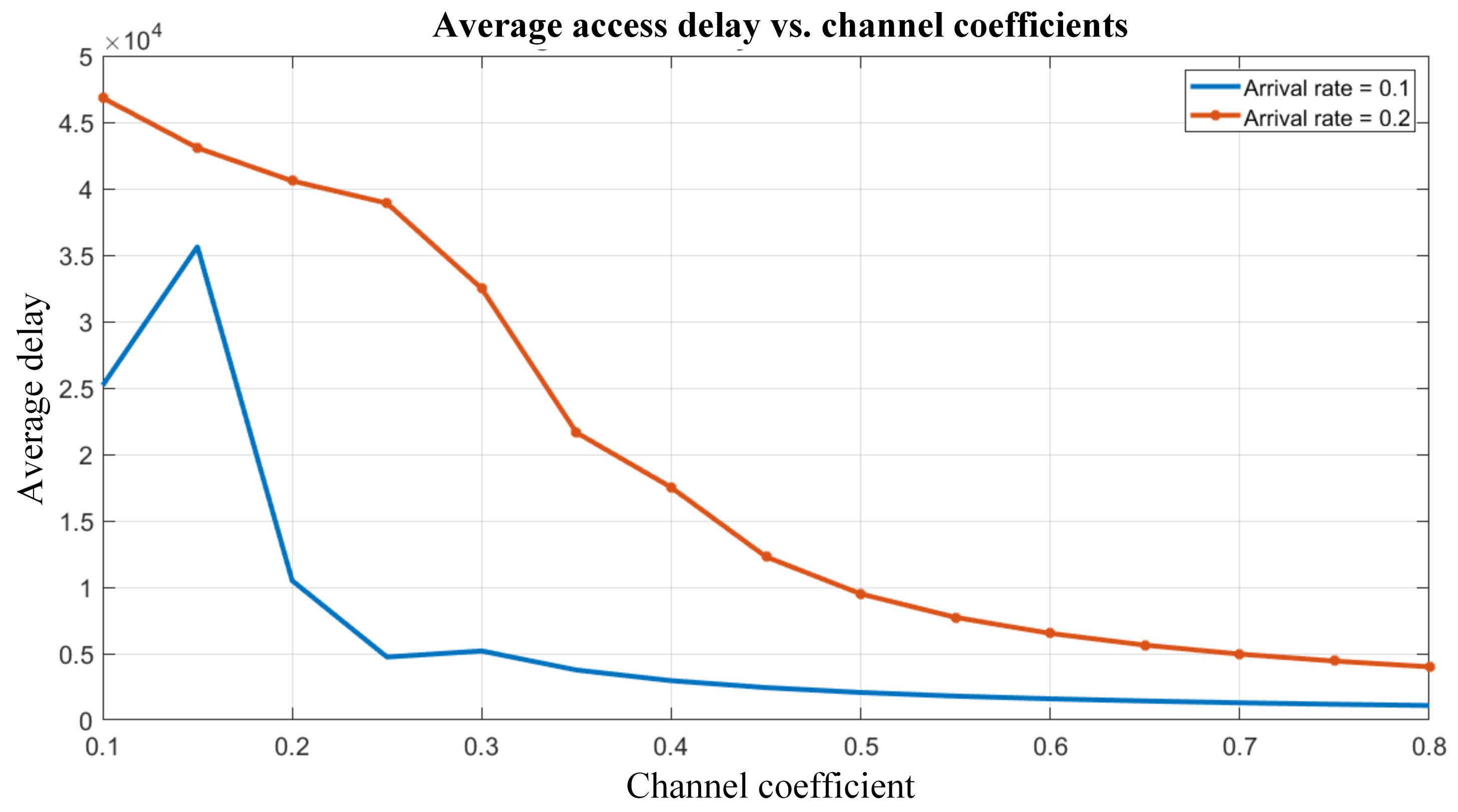
In Figure 8, we plotted the average access delay versus the channel coefficient while the arrival rate was kept constant. The access delays were plotted for two values of arrival rates, i.e., $\lambda =0.1,0.2$. It is obvious that the lower arrival rate exhibits a lesser access delay as shown in the figure. With an increasing value of channel coefficient, the average access delay decreases because larger values of the channel coefficient represent good channel conditions and vice versa.

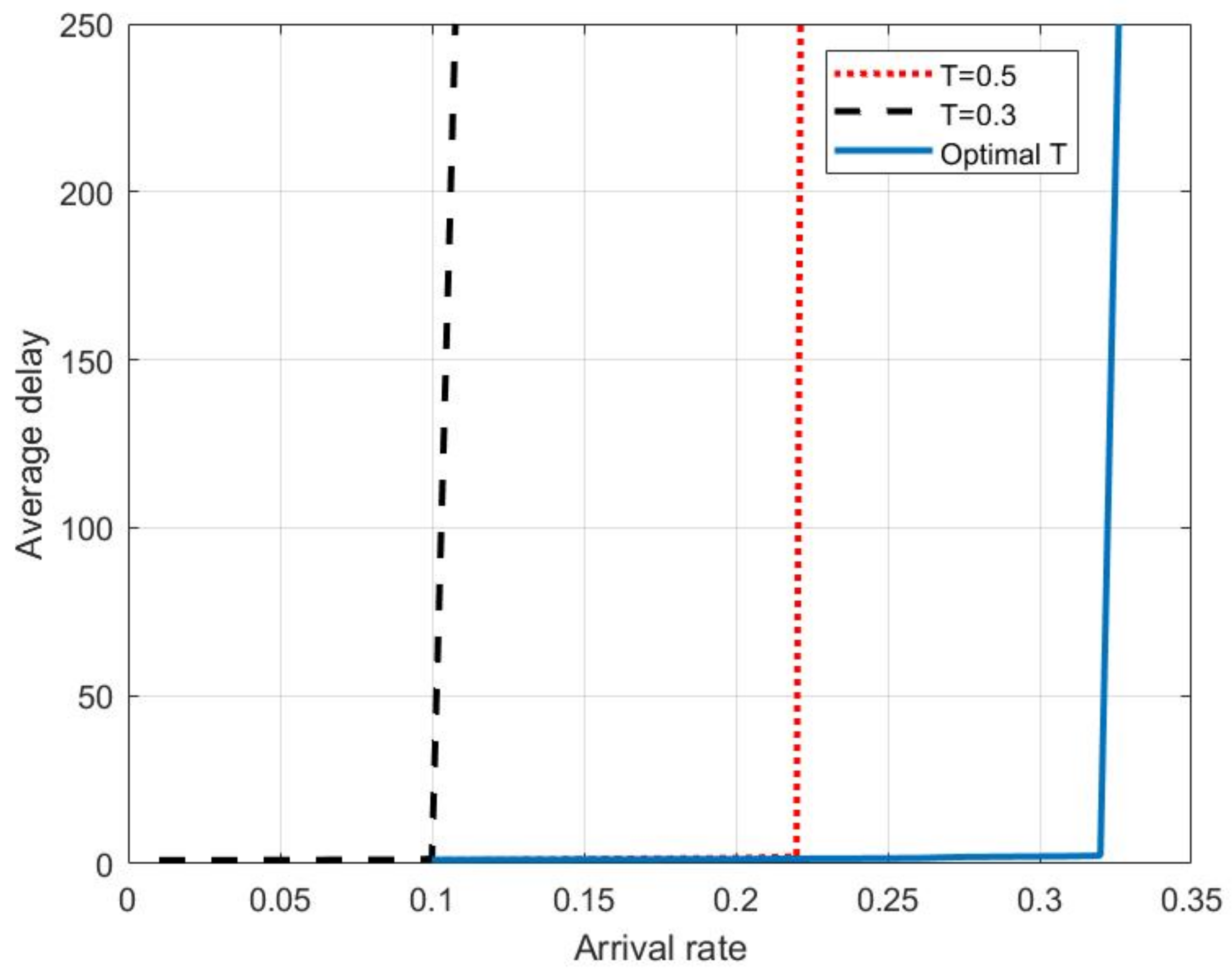
In Figure 9, we plotted the average access delay versus the arrival rate when the arrival rate varied from 0.1 to 0.3. The devices transmitted according to the scenario mentioned in Algorithm 1. We see that the access delay is small when the arrival rate is small and keeps on increasing with the increase of the arrival rate. This is understandable as more and more devices try to transmit to the channel when the arrival rate is large and hence, they need to wait more in the queues, which results in an increased access delay.

The plots in Figure 9 are shown for the scenarios where the thresholds on the channel coefficient are 0.3, 0.5, and the optimal T are represented in back, red, and blue colors, respectively. We see that when the threshold on the channel coefficient for transmission is 0.3 or 0.5, the average delay is large. This is because when the threshold is 0.3 and 0.5, too many devices transmit and this results in collisions, which increase the access delay. Similarly, when the threshold is optimal, a relatively fewer number of devices transmit, resulting in successful events. Moreover, it also reduces the number of idle events, and we see that when it is optimal, the delay is less as compared to 0.3 and 0.5.

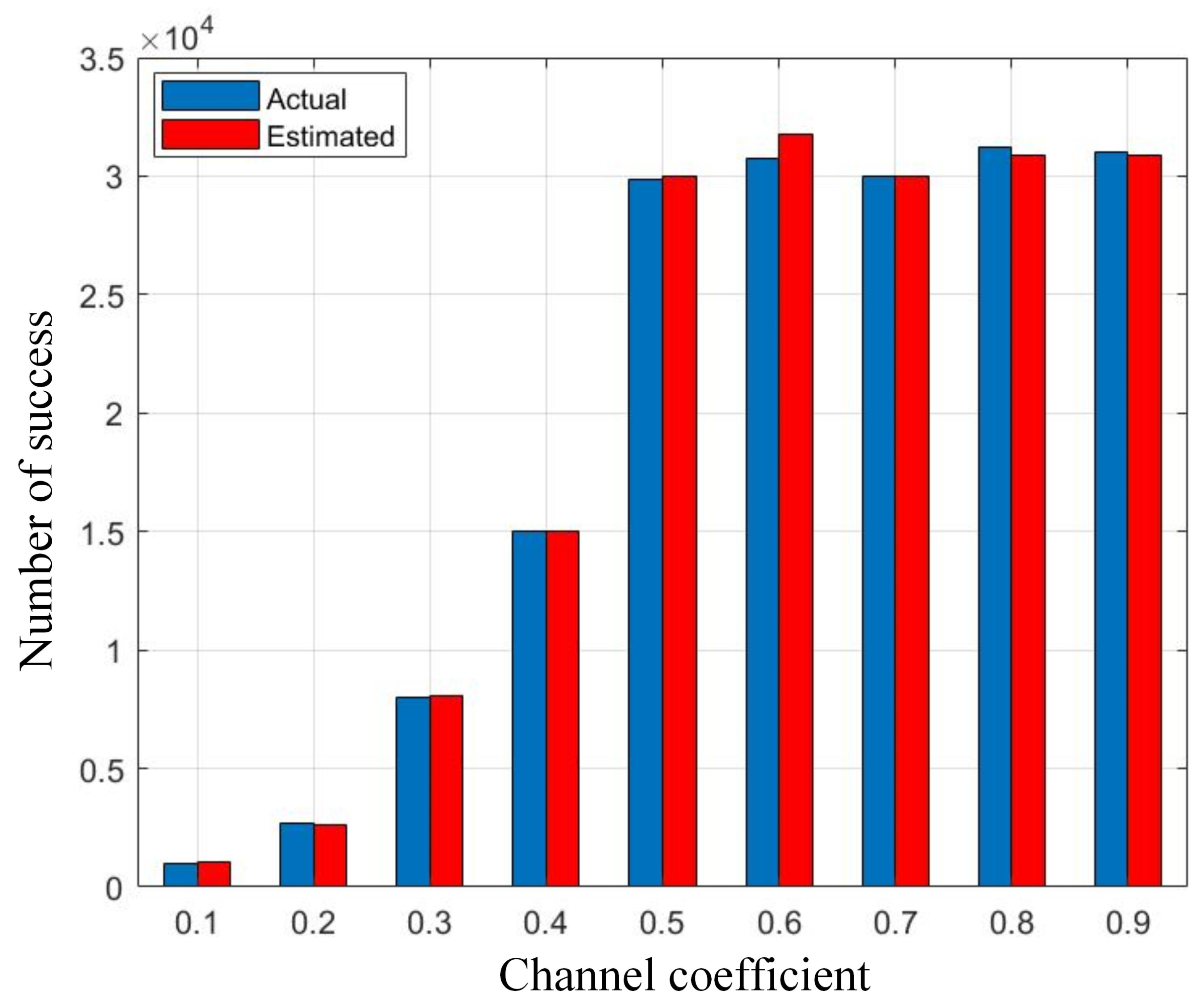
In Figure 10, we plotted the number of successes versus the channel coefficient threshold for the arrival rate of 0.2. We see that the number of successes is small when the threshold is low. It is because a large number of devices qualify for the transmission and it results in collisions.

As the threshold increases, a smaller number of devices transmit, thus increasing the chance of success. At the thresholds of zero and one, there is no success because the channel coefficients are generated in (0, 1), so no device qualifies for transmission, hence zero success. Moreover, we also plotted the number of successes in a scenario where the transmitting device was predicted through the DNN. The graph in blue color represents the actual number of successes whereas the estimated one in red color closely follows the actual ones. This shows that our algorithm works fine and that the DNN predicts the transmitting device such that success is maximized.

In Figure 11, we plotted the backlog of each station in actual and DNN-applied scenarios. The backlog at each station is the number of IoT devices waiting for transmission. In the actual scenario, the devices transmitted based on the Algorithm defined above for learning purposes. In the applied DNN scenario, the devices transmitted based on the prediction by the DNN. Please note that the DNN predicted which device needed to transmit to have maximum chances of success. We see that the backlogs of both scenarios are close to each other. Moreover, the backlog in the applied DNN scenario follows the actual backlog, which determines that the prediction is quite good and the actual scenario coincides with the applied DNN scenario.

Along the same lines as Figure 11, Figure 12 represents how the DNN erroneously selected a different device other than the actual one. In this figure, we present whether the DNN successfully predicts the transmitting device not. Since in each time slot, only one device transmits, the graph is either one or zero with one representing the transmission of a device and zero representing the idle scenario. We see that our DNN model performs correctly as we advance in time because we do not have a match in only some instances. We also observe that the DNN estimated graph closely follows the actual one which states that the DNN is performing well.

8. Conclusions and Future Works

The conventional LTE-A random access procedure uses an access-barring scheme to control congestion that arises due to a large number of IoT devices. This induces extra delay during the transmission, and the overall efficiency of the system is affected. This paper dealt with the grant-free transmission of IoT devices and coping with the collision problem which is associated with it. The paper proposed an efficient algorithm that took channel conditions into account and managed the transmission such that the successes were maximum and the collisions were minimum. The algorithm was used to train a DNN model using an optimal threshold and then the DNN model was used to predict which device needed to transmit to have maximum chances of success. We see that by using the proposed algorithm in grant-free transmission, the delay can be reduced and the overall system efficiency can be increased. As machine/deep learning can be used to maximize the success rate, it can also be used in other issues in random access networks. One such example is choosing eNodeB in dense deployments such that the probability of success is maximum. Since the eNodeBs can be large in number in dense deployments and the available traffic of devices may not be uniform, it is possible that some eNodeBs face sever congestion while others may not have any traffic. If the devices do not select the eNodeB intelligently, they may end up facing long queuing delays and consequently have less throughput. We observe that the devised algorithm selected the eNodeB such that the probability of success was maximum and hence it improved the overall efficiency of the system. So this algorithm can help alleviate congestion issues in dense deployment scenarios.

There can be different directions in which the work related to this topic can be done in the future. One research direction can be to prioritize the access of devices based on their importance using machine/deep learning. Currently, ACB is widely used as an access-barring technique and the devices compete for the transmission. However, there are certain devices which have time-critical data such as banks, hospitals, etc. A large delay can hinder their performance. Therefore, an algorithm can be devised to set the priorities of the devices and transmissions can be made based on the proposed algorithm such that the throughput is maximum, and the access delay of time-critical devices is minimum. Machine/deep learning can be used to predict the traffic of certain prioritized classes and the traffic can be routed to more lightly loaded eNodeBs in case of congestion. Different machine/deep learning techniques can also be used to select the best among them.

Another research direction can be to increase the throughput in grant-free random access, and again, machine/deep learning can help to solve the problem. Currently the transmission in random access is orthogonal, i.e., only one device can transmit on one channel in a given time and frequency resource. If more than one of the devices transmit on the same channel, it results in a collision, i.e., the receiver is unable to decode the transmission of each of the transmitting devices. Nonorthogonal transmission can be a solution to the problem where instead of taking it as a loss, it can be thought of as an advantage, and deliberately, more than one of the devices transmit on a single channel. At the receiving end, the receiver decodes the transmission of each of the transmitting devices using machine/deep learning. Based on the available parameters, machine/deep learning can help the receivers in decoding the received signals.