Smart-Median: A New Real-Time Algorithm for Smoothing Singing Pitch Contours

Featured Application

Some of the applications of this study are improving pitch estimation, removing outliers and errors, singing analysis, voice analysis, singing assessment, and singing information retrieval.

Abstract

Pitch detection is usually one of the fundamental steps in audio signal processing. However, it is common for pitch detectors to estimate a portion of the fundamental frequencies incorrectly, especially in real-time environments and when applied to singing. Therefore, the estimated pitch contour usually has errors. To remove these errors, a contour smoother algorithm should be employed. However, because none of the current contour-smoother algorithms has been explicitly designed to be applied to contours generated from singing, they are often unsuitable for this purpose. Therefore, this article aims to introduce a new smoother algorithm that rectifies this. The proposed smoother algorithm is compared with 15 other smoother algorithms over approximately 2700 pitch contours. Four metrics were used for the comparison. According to all the metrics, the proposed algorithm could smooth the contours more accurately than other algorithms. A distinct conclusion is that smoother algorithms should be designed according to the contour type and the result’s final applications.

1. Introduction

Estimating the fundamental frequency is usually one of the main steps in audio signal processing algorithms. However, it is common for pitch detector algorithms to make some incorrect estimations, resulting in a pitch contour that is not smooth and includes errors. These errors are often due to doubling or halving estimates of the true pitch value, and are therefore impulsive in appearance rather than random [1,2,3,4,5]. Furthermore, incorrect pitch estimation often happens in real-time pitch detection, especially when the sound source is a human voice [5]. Therefore, a contour-smoother algorithm is necessary to filter the incorrectly estimated F0 before further analysis.

Generally, contour smoothers can be divided into two categories: 1—contour smoothing to show the data trend; and 2—contour smoothing to remove errors, noise, and outlier points.

There are several algorithms for showing contour trend, such as polynomial [6], spline [7,8], Gaussian [9], Locally Weighted Scatterplot Smoothing (LOWESS) [10,11], and seasonal decomposition [12]. One of the applications of trend detection using pitch contours is to find the similarity between melodies [13,14,15,16]. Other contour smoothers, such as moving average [17] and Median filter, function by attenuating or removing outliers in the contour [5]. None of these contour-smoother algorithms was explicitly designed for smoothing pitch contours; they can be used for any contour from any data series. They have been applied to the smoothing of pitch contours, such as in the study by Kasi and Zahorian [18] that used the Median filter. However, there are certain adjusted versions of these algorithms for smoothing estimated pitches; for example, Okada et al. [19] and Jlassi et al. [20] introduced pitch contour algorithms based on the Median filter. In the following, some of these adjusted algorithms are discussed.

Zhao et al. [2] introduced a pitch smoothing method for the Mandarin language based on autocorrelation and cepstral F0 detection approaches. They first used two pitch estimation techniques to estimate two separate pitch contours, and then both were smoothed. Finally, combining the two estimated pitch contours created the smoothed contour. Generally, their approach was very similar to the idea of this paper, moving through a pitch contour to identify noisy estimates by comparing each point to its previous and succeeding points, and finally editing out the noise. However, their approach involved altering some correct parts of the data, which impacted peaks that were not incorrect. Moreover, in their evaluation, they only checked the error reduction capability of their algorithm for removing octave-doubling and sharp rises in estimated F0s. It would have been preferable to compare their smoothed contours with ground truth, to show how well their algorithm could adjust the estimated contour to make it similar to that of the ground truth.

Liu et al. [21] introduced a pitch-contour-smoother algorithm for Mandarin tone recognition. They used several thresholds for finding half, double, and triple errors by comparing each point with its previous point. Then, an incorrect frequency was doubled, halved, or divided by three, according to the type of error detected. They indicated that experiments should determine the threshold values, but did not provide any guidelines for selecting or adjusting these. In addition, the threshold values they used were not revealed. Therefore, it is unclear how one could change the thresholds to optimize the result. In addition, they tested their algorithm only on an isolated Mandarin syllabus, although realistically they should also have tried their approach on continuously spoken language. Moreover, they did not compare the accuracy of their algorithm with other contour-smoother algorithms to show how well their method performed compared to others.

The smoothing approach presented by Jlassi et al. [20] was designed for spoken English. Their smoothing system was based on the moving average filter. However, they only calculated the average of the two immediately previous F0 points for those points that showed more than a 30 Hz difference from their previous and following points. They compared their algorithm with the Median filter and Exponentially Weighted Moving Average (EWMA), and found improved accuracy using their approach. However, the dataset [22] used in their study was small (15 people reading a phonetically balanced text, “The North Wind Story”). Their results would have been much more convincing if they had evaluated their algorithm with a more extensive dataset generated by various pitch-detector algorithms. Moreover, several metrics could have been employed to measure how well they smoothed the errors. Furthermore, their algorithm considered a difference of more than 30 Hz from both the immediately previous and following points as an error; therefore, it was unable to identify and smooth any errors existing over more than one point on the contour.

Ferro and Tamburini [1] introduced another pitch-smoother technique for spoken English, based on Deep Neural Networks (DNN) and implemented explicitly as a Recurrent Neural Network (RNN). However, they did not provide a comparison between the improvement offered by their approach and that of any other method. In addition, comparison of their datasets and the mixture of datasets suggests that their DNN architecture may not work well with a new dataset.

As exemplified above, many pitch detection algorithms have been designed for and tested on speech. However, although both speech and singing are produced with the same human vocal system, because of the differences between speaking and singing, separate studies are required for pitch analysis of singing [23]. In addition, in real-time environments, the smoother algorithm should alter the contour with a reasonable delay, mainly based on previous data because future data is unavailable.

We believe that the smoother algorithm should be based on the features and applications of the contour, similar to the approach taken by Ferro and Tamburini [1] and the studies by So et al. [3] on smoothing contours generated from speech. In other words, expected error types in the pitch contours for the specific data type should be identified. Then, an investigation for a targeted contour-smoother algorithm to solve these errors should be made. In addition, the applications of the smoothed contour should also be considered. For example, when a highly accurate estimate of the F0 value at each point is required, the smoother algorithm should not change any data except those points identified as incorrectly estimated. Moreover, in real-time environments the smoother algorithm should not have a long delay.

This paper, therefore, introduces a new contour-smoother algorithm based on the features and applications of pitch contours that are derived only from singing. For this purpose, after describing the methodology applied, several typical contour-smoother algorithms are described. Then, the proposed algorithm is explained in Section 4, followed by the results and discussion. Finally, a conclusion and suggestions for future work are provided in Section 7.

2. Materials and Methods

2.1. Dataset

The VocalSet dataset [24] was used to evaluate the algorithms’ accuracy. This dataset includes more than 10 h of recordings of 20 (11 males and 9 females) professional singers. VocalSet includes a complete set of vowels and a diverse set of voices that exhibit many different vocal techniques, singing in contexts of scales, arpeggios, long tones, and melodic excerpts. For this study, a portion of VocalSet was selected; the scales and arpeggios sung across the vowels in loud slow and fast performances. The total number of files used from VocalSet was 511.

2.2. Ground Truth

In order to evaluate the accuracy of each of the smoother algorithms, ground truth pitch contours were required to compare the smoothed pitch contours. In other words, in this study, the best smoothing algorithm was considered the one that produced contours most similar to the ground truth. According to studies by Faghih and Timoney [4,5], a reliable offline pitch detector algorithm called PYin [24] was used. The pitch contours estimated by PYin were saved in several CSV files with two columns, time in seconds and F0. These were all plotted to ensure the accuracy of the pitch contours estimated by PYin. Those that included irrational jumps were considered incorrect and deleted. Therefore, after removing those contours, the number of the ground truth files remaining was 447.

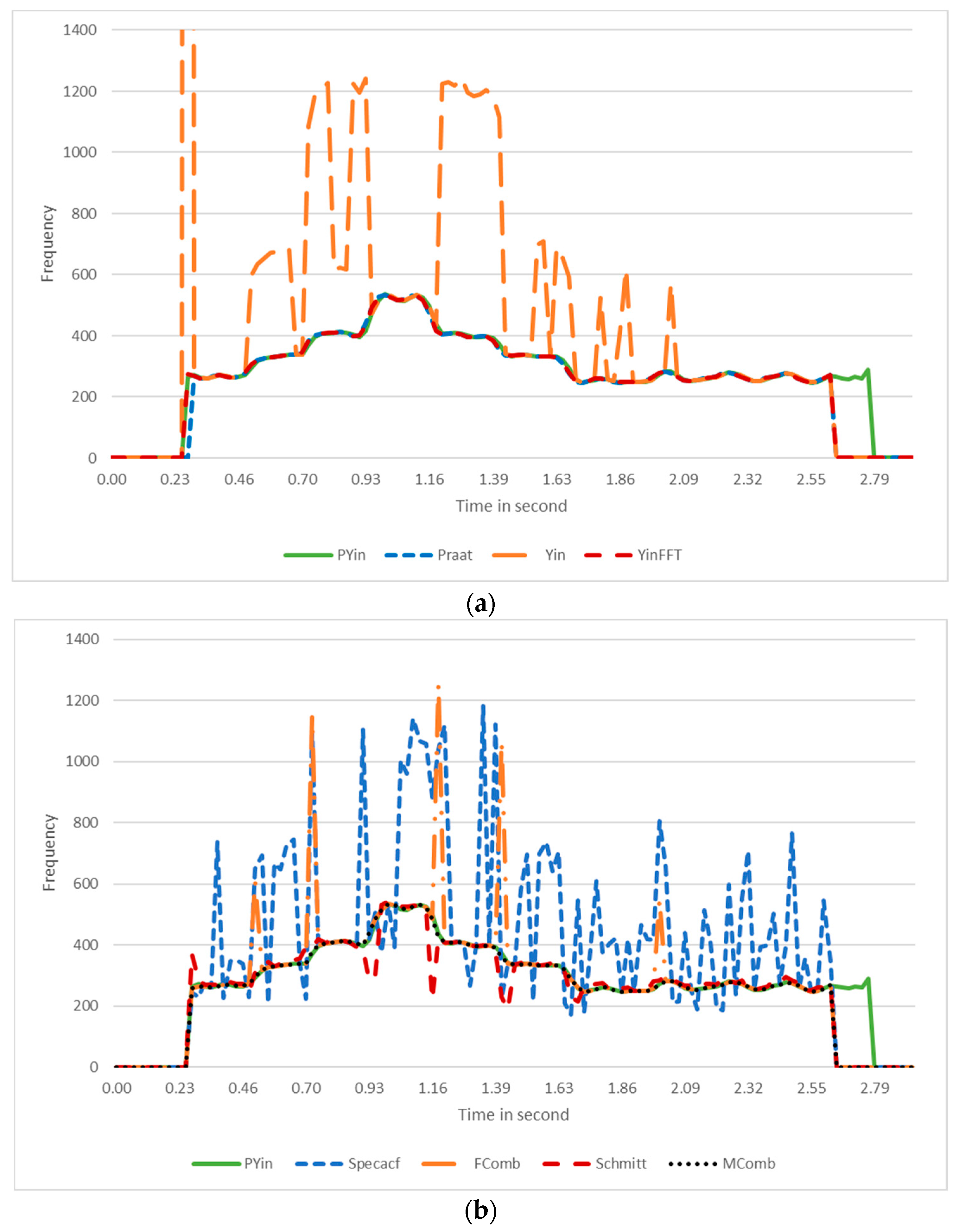
2.3. Pitch Detection Algorithms to Generate Pitch Contours

To evaluate the proposed smoother algorithm, we used a similar approach as [1], employing several pitch contours with different random error (unsmoothed) points. As Faghih and Timoney’s [5] study discussed, six real-time pitch detection algorithms with different estimated contours were employed to obtain the required contours. The pitch detector algorithms were Yin [25], spectral YIN or YIN Fast Fourier transform (YinFFT), Fast comb spectral model (FComb), Multi-comb spectral filtering (Mcomb), Schmitt trigger, and the spectral auto-correlation function (specacf). The implementation for these algorithms came from a Python library, Aubio (https://aubio.org/manual/latest/cli.html#aubiopitch, accessed on 10 June 2021) [26], a well-known library for music information retrieval. Since the focus of this paper is on smoothing pitch contours, descriptions of these algorithms are not provided in this paper but can be found in [5,27]. The reason for selecting these real-time pitch estimators was that, based on the study by Faghih and Timoney [5], none of them can estimate F0s without error in singing signals. In addition, the accuracy of these algorithms varies, which helped us evaluate the contour-smoother algorithms in different situations.

In addition, to compare the accuracy of the algorithms in conditions where the pitch contours included no or only a few errors, an offline pitch-detector algorithm provided in the Praat tool [28] based on the Boersma algorithm [29] was used. According to Faghih and Timoney’s studies [4,5], the Praat and Pyin accuracies tend to be similar.

The settings used for pitch detection for women’s voices were 44,100 for sample rate, 1024 for window size, and 512 for hop size. The related settings for men’s voices were 44,100, 2048, and 1024 for sample rate, window size, and hop size, respectively. Therefore, the distance between two consecutive points in a pitch contour for women’s voices was 11.61 milliseconds, and for men’s voices was 23.22 milliseconds.

As shown in Figure 1, the contours generated by the different pitch detectors exhibited various errors. Therefore, the total number of contours used to evaluate the smoother algorithms was 2682 (corresponding to the six pitch detectors run on each of the 447 wav files).

All the provided files, such as the dataset and codes, are available in a GitHub repository at https://github.com/BehnamFaghihMusicTech/Smart-Median, accessed on 6 July 2022.

2.4. Evaluation Method

Several evaluation metrics were used to compare the accuracy of the smoothing algorithms. The metrics used for the evaluations were R-squared (R²), Root-Mean-Square Error (RMSE), Mean-Absolute-Error (MAE), and F0 Frame Error (FFE). A well-known Python library called Sklearn [30] was used for the metrics, except for the FFE metric that was created by this paper’s authors. These metrics are explained in the following subsections.

2.4.1. R-Squared (R²)

The formula for this metric is as follows (1) [31]:

$$R^2=1-\frac{{{\displaystyle \sum }}_{i=1}^N{\left(G{T}_i-S{M}_i\right)}^2}{{{\displaystyle \sum }}_{i=1}^N{\left(G{T}_i-mean\left(GT\right)\right)}^2}=1-\frac{\mathrm{Regression}\mathrm{Sum}\mathrm{of}\mathrm{Squares}\left(RSS\right)}{\mathrm{Total}\mathrm{Sum}\mathrm{of}\mathrm{Squares}\left(TSS\right)}$$

(1)

where $N$ is the total number of frames, $GT$ is the ground truth contour, $SM$ is the smoothed contour, and the $mean\left(GT\right)=\frac{1}{N}{\displaystyle \sum }_{i=1}^{N}G{T}_i$.

In the best case, when all the points in the ground truth contour and the estimated contour are similar, $R^2$ is equal to 1; otherwise, $R^2$ is less than 1. A value closer to 1 means more similarity between the two contours.

2.4.2. Root-Mean-Square Error (RMSE)

This metric is calculated according to the following Formula (2):

$$RMSE=\sqrt[2]{\frac{{{\displaystyle \sum }}_{i=1}^N{\left(G{T}_i-S{M}_i\right)}^2}{N}}$$

(2)

In the best case, when the two contours have precisely the same values, the RMSE is 0; otherwise, it is more significant than 0. Closer values to 0 mean more similarity between two contours.

2.4.3. Mean-Absolute-Error (MAE)

Equation (3) shows how to calculate this metric:

$$MAE=\frac{{{\displaystyle \sum }}_{i=1}^N\mid G{T}_i-S{M}_i\mid }{N}$$

(3)

MAE is similar to RMSE, but, because of the squared difference, RMSE can be considered a more significant penalty for points at a greater distance from corresponding points in the ground truth contour.

2.4.4. F0 Frame Error (FFE)

FFE is the proportion of frames within which an error is made. Therefore, FFE alone can provide an overall performance measure of the accuracy of the pitch detection algorithm [32]. This metric calculates the percentage of points in the estimated pitch contour that are within a Threshold distance of corresponding points in the ground truth pitch contour (4):

$$FFE=\frac{{{\displaystyle \sum }}_{i=0}^N\{\begin{array}{c}1\left|\frac{S{M}_i}{G{t}_i}\right|\le Threshold\\ 0otherwise\end{array}}{N}\times 100$$

(4)

where $N$ is the total number of frames/points.

For the $Threshold$, in studies such as [1], a constant value, e.g., 16 Hz, was used as an acceptable variation from the ground truth. However, as is discussed by Faghih and Timoney [5], a fixed distance from the ground truth may not be a good approach, because the perceptual effect of 16 Hz is different when the estimated pitch is 100 Hz compared to 1000 Hz. However, it is also common to use a percentage, usually 20%, as the threshold [20], and a similar approach is used in this study.

Higher values of this metric indicate a higher similarity between the smoothed pitch contour and the ground truth pitch contour.

It should be mentioned that there are other algorithms for finding the similarities between pitch contours, such as those of Sampaio [13], Wu [14], and Lin et al. [15]. However, these aim to determine perceptual similarity between two pitch contours. In other words, those researchers were seeking to determine the similarity of one melody to another. The purpose of the current paper is not to ascertain the overall similarities between two tunes, but rather the numerical relationship between each point on two different pitch contours. Therefore, those algorithms were not suitable for this study.

3. Current Contour Smoother Algorithms

Several contour-smoother algorithms are commonly used to smooth pitch contours. This section provides a list of these algorithms.

To refer to the smoother algorithms within this paper, a code has been assigned to each algorithm listed in

Table 1. Code of each of the contour smoother algorithms.

Code	Algorithm
00	Smart-Median
01	Gaussian (sigma = 1)
02	Savitzky–Golay filter
03	Exponential
04	Window-based (window_type = ‘rectangular’)
05	Window-based (window_type = ‘hanning’)
06	Window-based (window_type = ‘hamming’)
07	Window-based (window_type = ‘bartlett’)
08	Window-based (window_type = ‘blackman’)
09	Direct Spectral
10	Polynomial
11	Spline (type = ‘linear_spline’)
12	Spline (type = ‘cubic_spline’)
13	Spline (type = ‘natural_cubic_spline’)
14	Gaussian (sigma = 0.2, n_knots = 10)
15	Binner
16	LOWESS
17	Decompose (type = ‘Window-based’, method = ‘additive’)
18	Decompose (type = ‘lowess’, method = ‘additive’)
19	Decompose (type = ‘natural_cubic_spline’, method = ‘additive’)
20	Decompose (type = ‘natural_cubic_spline’, method = ‘multiplicative’)
21	Decompose (type = ‘lowess’, method = ‘multiplicative’)
22	Decompose (type = ‘natural_cubic_spline’, method = ‘multiplicative’)
23	Kalman (component = ‘level’)
24	Kalman (component = ‘level_trend’)
25	Kalman (component = ‘level_season’)
26	Kalman (component = ‘level_trend_season’)
27	Kalman (component = ‘level_longseason’)
28	Kalman (component = ‘level_trend_longseason’)
29	Kalman (component = ‘level_season_longseason’)
30	Kalman (component = ‘level_trend_season_longseason’)
31	Moving Average (simple = True)
32	Moving Average (simple = False)
33	Median Filter
34	Okada Filter
35	Jlassi Filter

.

Figure 2 illustrates the effect of the smoother algorithms on a single estimated pitch contour. A female singer sang an arpeggio in the C major scale, and the FComb algorithm estimated the pitches. The smoothed contours are plotted in eight different panels. Each panel includes ground truth (GT), the original estimated (ST) contours, and the smoothed contours generated by some of the smoother algorithms.

In addition, the Python libraries employed to implement these smoothers are listed in Appendix A.

Each of the algorithms is described below.

3.1. Gaussian Filter

Generally, in signal processing, filtering removes or modifies unwanted error and noise signals from a series of data. Therefore, Gaussian filters smooth out fluctuations in data by convolution with a Gaussian function [9]. The one-dimensional Gaussian filter is expressed as (5):

$$S{m}_i=\frac{1}{\sqrt{2\pi \sigma }}\exp \left(-\frac{{\left(E{s}_i\right)}^2}{2{\sigma }^2}\right)$$

(5)

where $E{s}_i$ is the original signal at position $i$, and $S{m}_i$ is the smoothed signal at position $i$. In addition, ${\sigma }^2$ indicates the variance of the Gaussian filter. The smoothing degree depends on the variance value size [9]. Although the Gaussian filter smooths out the noise, as shown in Figure 2a, some correctly estimated F0 may also change, i.e., become distorted [9].

3.2. Savitzky–Golay Filter

This particular type of low-pass filter was introduced into analytical chemistry, but soon found many applications in other fields [33]. It can be considered a weighted moving average [34], and is defined as follows (6):

$$S{m}_i={\displaystyle \sum }_{k=-M}^M{h}_{k}E{s}_{i-k}$$

(6)

where $E{s}_i$ is the original signal at position $i$, and $S{m}_i$ is the smoothed signal at position $i$. $M$ is window length and $h_k$ are the filter coefficients that indicate the boundaries of the data. The drawback of the Savitzky–Golay (SG) filter, according to Schmid et al. [35], is that the data near the edges is prone to artefacts. Figure 2a illustrates its effect on a contour.

3.3. Exponential Filter

This approach is based on weighting the current values by the previously observed data, assuming that the most recent observations are more important than the older ones. The smoothed series starts with the second point in the contour. It is calculated by [36], (7):

$$S{m}_i=\alpha E{s}_{i-1}+\left(1-\alpha \right)S{m}_{i-1}0<\alpha \le 1\mathrm{i}\ge 3.$$

(7)

where $\alpha$ is called the smoothing constant. An illustration of this smoothing effect can be seen in Figure 2a.

3.4. Window-Based Finite Impulse Response Filter

In this approach, a window works as a mask to filter the data series. Different window shapes can be considered for filtering data. Each window point is usually between 0 and 1. Therefore, this method uses weighted windows. If $E{s}_i$ is considered a signal at index $i$, and a window at index $i$ as $w_i$, the smoothed signal $S{m}_i$ is calculated as follows, (8):

$$S{m}_i=w_{i}E{s}_i$$

(8)

The window types used in this study are described below.

3.4.1. Rectangular Window

This means that the window’s values all equal one; Figure 2b.

3.4.2. Hanning Window

The Hanning window is defined as follows, from [37] (9):

$$W_H\left(i\right)=\{\begin{array}{c}0.5\left[1-\cos \left(2\pi \frac{i}{N}\right)\right]\\ 0otherwise\end{array}0\le i=N-1$$

(9)

where $N$ is the length of the window; Figure 2b.

3.4.3. Hamming Window

The Hamming window is defined as follows, from [37] (10):

$$w_{HM}\left(i\right)=\{\begin{array}{c}0.54+0.46\cos \left(2\pi \frac{i}{N}\right)0\le n\le N-1\\ 0otherwise\end{array}$$

(10)

where $N$ is the length of the window; Figure 2b.

3.4.4. Bartlett Window

The Bartlett (triangular) window is defined [37] using (11), Figure 2b:

$$w_b\left(i\right)=\{\begin{array}{c}10\le i\le N-1\\ 0otherwise\end{array}$$

(11)

3.4.5. Blackman Window

The Blackman window is defined [38] by (12):

$$w_{black}\left(i\right)=a_0+a_1+a_2\cos \frac{4\pi i}{N-1}for-\frac{N-1}{2}\le i\le \frac{N-1}{2}$$

(12)

where $N$ is the window length, and $a_0,a_1\mathrm{and}{a}_2$ are constants (13):

$$a_0=\frac{1-\alpha }{2},a_1=\frac{1}{2},a_2=\alpha /2$$

(13)

The $\alpha$ is static, and equals $0.16$; Figure 2c.

3.5. Direct Spectral Filter

In this approach, a time series is smoothed by employing a Fourier Transformation. The essential frequencies remain, and others are removed. It operates similarly to multiplying the frequency domain by a rectangular window. In other words, it is a circular convolution generated by transforming the window in the time domain; Figure 2c.

3.6. Polynomial

This approach uses weighted linear regression on an ad-hoc expansion basis to smooth the time series. It is a generalization of the Finite Impulse Response (FIR) filter that can better preserve the desired signal’s higher frequency content without removing as much noise as the average [39]. The first derivative of the polynomial evaluated at the midpoint of the N-interval is generated by multiplying the position data $E{s}_i$ by coefficients and adding these multiplications, as shown in (14) [6]:

$$S{m}_{\left(N+1\right)/2}={\displaystyle \sum }_{i=1}^N{W}_{i}E{s}_i\left(N=\mathrm{number}\mathrm{of}\mathrm{data}\mathrm{points}\left(\mathrm{odd}\right)\right)$$

(14)

where $W_i$ are the weights (coefficients) of the polynomial fit of degree $p$. The weights depend on the degree $p,$ and the number of points, N, used in the fit; Figure 2c is an example.

3.7. Spline

This approach employs Spline functions to eliminate the noise from the data. It works by estimating the optimum amount of smoothing required for the data. Three types of spline smoothing were used in this study: ‘linear’ (Figure 2c), ‘cubic’ (Figure 2d), and ‘natural cubic’ (Figure 2d). The details of this approach are provided in [7,8].

3.8. Binner

This approach applies linear regression on an ad-hoc expansion basis within a time series. The features created by this method are obtained via binning the input space into intervals. An indicator feature is designed for each bin, indicating into which bin a given observation falls. The input space consists of a single continuous increasing sequence in the time series domain [40]; an illustration is shown in Figure 2d.

3.9. Locally Weighted Scatterplot Smoothing (LOWESS) Smoother

This is a non-parametric regression method. LOWESS attempts to fit a linear model to each data point, based on local data points; Figure 2e. This makes the procedure more versatile than simply including a high-order polynomial [10,11].

3.10. Seasonal Decomposition

One of the considerations in analysing time series data is dealing with seasonality. A seasonal decomposition deconstructs a time series into several components: a trend, a repeating seasonal time series, and the remainder. One of the benefits of seasonal decomposition is its capacity to locate anomalies and errors in data [12]. Seasonal decomposition can estimate the notes and seasons in a pitch contour, but the vibrations sung in each note are removed. Therefore, it can show the movements between seasons and notes in a pitch contour, as shown in Figure 2e,f.

Two seasonal component assessments may be used: ‘additive’ and ‘multiplicative’. In the additive method, the variables are assumed to be mutually independent and calculated by summation of the variables. The multiplicative approach considers that components are dependent on each other, and it is calculated by the multiplication of the variables [41].

Seasonal decomposition can be employed using different smoothing techniques. The smoothing techniques used in this study are Window-based, ‘LOWESS’, and ‘natural_cubic_spline’.

3.11. Kalman Filter

The Kalman filter is a set of mathematical equations that provides an efficient recursive means to estimate the state of a process in a way that minimises the norm of the squared error. The Kalman filter uses a form of feedback control, assessing the process state and then obtaining feedback in the form of (noisy) measurements. The equations for the Kalman filter have two parts: time update equations and measurement update equations. The time update equations operate as predictor equations, while the measurement update equations are corrector equations. Thus, the overall estimation algorithm is close to a predictor–corrector algorithm, i.e., correcting to improve the predicted value. In the standard Kalman filter, it is assumed that the noise is Gaussian, which may or may not reflect the reality of the system that is being modelled [42]. Thus, the more accurate the model used in the Kalman algorithm, the better the performance.

The Kalman smoother can be represented in the state space form. Therefore, a matrix representation of all the components is required. Four structure presentations in the contours are considered: ‘level’, ‘trend’, ‘seasonality’ and ‘long seasonality’, and a combination of these structures can be considered. Examples of the effects of different variations of the Kalman filter are shown in Figure 2f,g.

3.12. Moving Average

This simple filter aims to reduce random noise in a data series [17] by following the Formula (15):

$$S{m}_i=\frac{1}{n}{\displaystyle \sum }_{j=0}^{n-1}E{s}_{i+j}$$

(15)

where $Es$ is the original pitch contour, $Sm$ is the smoothed pitch contour, and $n$ is the number of points analysed at any given time and is referred to as the window length of the filter. The larger the value of n, the greater the level of smoothing. An example can be seen in Figure 2h.

3.13. Median Filter

The Median filter approach is similar to the moving average. Still, instead of calculating the average of a window of length n, the Median of the window is considered (16). Unlike the moving average filter, which is a linear system, this filter is nonlinear, rendering a more complicated analysis:

$$S{m}_i=Median\left(E{s}_i,E{s}_{i+1},E{s}_{i+2},\dots ,E{s}_{i+n-2},E{s}_{i+n-1}\right)$$

(16)

where $Es$ is the original pitch contour, $Sm$ is the smoothed pitch contour, and $n$ is the number of points to calculate the Median at each instant. Figure 2h illustrates the effect of this method.

3.14. Okada Filter

This filter is an exciting combination of moving average and Median filter. This filter aims to remove the outliers from a contour while closely retaining its shape, by not incurring softening of contour definition at transitions typically observed with smoothing. Each of the estimated points $E{s}_i$ in a contour is compared with its immediate previous and successive points, $E{s}_{i-1}\mathrm{and}E{s}_{i+1}$, respectively. If $E{s}_i$ is the median of $E{s}_{i-1},E{s}_i,$ and $E{s}_{i+1}$, then it does not need to be changed, otherwise $E{s}_i$ will be replaced by the average of $E{s}_{i-1}\mathrm{and}E{s}_{i+1}$, as shown in (17). In this case, the first and the last point will not be changed [19].

$$S{m}_i=E{s}_i+\frac{E{s}_{i-1}+E{s}_{i+1}-2E{s}_i}{2\left(1+e^{-\alpha \left(E{s}_i-E{s}_{i-1})(E{s}_i-E{s}_{i+1}\right)}\right)}$$

(17)

When α is sufficiently large, it can perform two operations: (1) if $\left(E{s}_i-E{s}_{i-1})(E{s}_i-E{s}_{i+1}\right)\le 0$, $E{s}_i$ is assigned to $S{m}_i$; and (2) if $\left(E{s}_i-E{s}_{i-1})(E{s}_i-E{s}_{i+1}\right)>0$, $S{m}_i$ is assigned by $\left(E{s}_{i-1}+E{s}_{i+1}\right)/2$.

Figure 2h provides an example of this algorithm effect.

3.15. Jlassi Filter

This technique was presented by Jlassi et al. [20]. This approach has two main steps, first, finding the incorrect points in the pitch contour by considering those that exhibit a difference of more than a set threshold from both their previous and successive points. Second, replacing the incorrect point with the average of the last two points (18):

$$S{m}_i=\{\begin{array}{c}\frac{E{s}_{i-2}+E{s}_{i-1}}{2}\left|E{s}_i-E{s}_{i-1}\right|>Thresholdand\left|E{s}_i-E{s}_{i+1}\right|>Threshold\\ E{s}_{i}otherwise\end{array}$$

(18)

The value for $Threshold$ is assumed to be 30, as mentioned in the original paper. Figure 2h illustrates the effect of the algorithm.

4. Smart-Median: A Real-Time Pitch Contour Smoother Algorithm

The approach applied in this study to adjust the incorrectly determined pitch values was based on the Median method, and has been named Smart-Median. The Smart-Median method is based on the belief that each contour should be smoothed based on its data features and intended applications. In other words, a general contour smoother may not be suitable for all applications. The considerations for designing the Smart-Median are given below.

4.1. Considerations

The Smart-Median algorithm is based on the following considerations:

• Only the incorrectly estimated pitches need to be changed. Therefore, it is necessary to decide which jumps in a contour are incorrect.
• To calculate the median, some of the estimated pitches around the incorrectly detected F0 should be selected. This represents the window length for calculating the median. Therefore, the decision on the number of estimated pitches before and/or after the erroneously estimated pitches provides the median window length. Thus, a delay is required in real-time scenarios to ensure sufficient successive pitch frequencies are available when correcting the current pitch frequency.
• There is a minimum duration for which a human can sing.
• There is a minimum duration for which a human can rest between singing two notes.
• There is a maximum frequency that a human can sing
• There is a maximum interval during which humans can move from one note to another when singing.
• A large pitch interval in a very short time is impossible.

The following section explains our decisions regarding each of the above considerations.

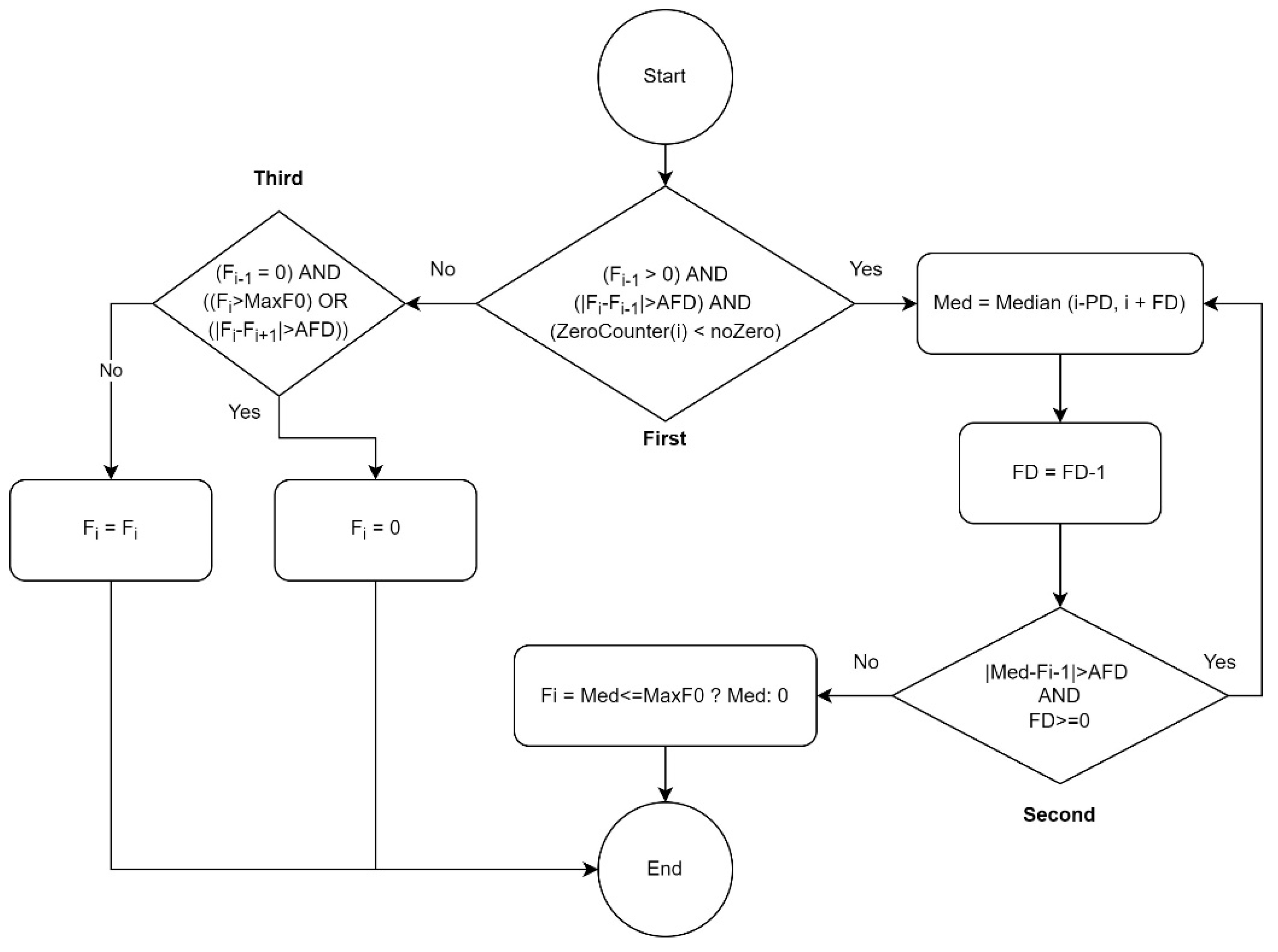
4.2. Smart-Median Algorithm

The flowchart shown in Figure 3 illustrates how incorrectly estimated pitches can be distinguished. In addition, it indicates which estimated pitches should be selected to calculate the median for the wrongly detected pitches.

There are several variables and functions in the flowchart, explained as follows:

• F_i refers to the frequency at index i.
• AFD (Acceptable Frequency Difference) indicates the maximum pitch frequency interval acceptable for jumping between two consequent detected pitches. In two studies on speech contour-smoother algorithms [2,20], 30 Hz was selected as the AFD according to the researchers’ experiences. Because the frequency range that humans use for singing is wider than for speaking, a larger AFD is needed for singing. According to the dataset used, the largest interval between two consequently notes sung by men was from C4 to F4, at frequencies of approximately 261 Hz and 349 Hz, respectively, so the maximum interval was 88 Hz for men. The largest interval between notes sung by women was C5 to F5, at frequencies of approximately 523 Hz and 698 Hz, respectively. Therefore, the biggest interval for women was 175 Hz. According to our observations of pitch contours, the human voice cannot physically produce such a big jump within a 30 ms timestep; i.e., for moving from C4 to F4 or from C5 to F5, more than 30 ms is needed. Therefore, it was found that an AFD with a value of 75 Hz was an acceptable choice for pitch contours comprised mostly of frequencies less than 300 Hz (male voices). For those with frequencies that mostly greater than 300 Hz (female singers), 110 Hz was a good choice of AFD.
• noZero: this is the minimum number of consequent zero pitch frequencies that should be considered a correctly estimated silence or rest. In this study, 50 milliseconds was regarded as the minimum duration for silence to be accepted as correct [43]; otherwise, the silence requires adjustment to the local median value.
• The ZeroCounter(i) method calculates how many frequencies (pitches) of zero value exist after index i. The reason for checking the number of zero values (silence) is to ascertain whether or not the pitch detector algorithm has estimated a region of silence correctly or in error.
• Median(i,j): calculates the median based on pitch frequencies from index i to index j.
• PD (Prior Distance): this indicates how many estimated pitches before the current pitch frequency should be considered for the median. In this study, the PD was calculated to cover three estimated pitch frequencies, approximately 35 and 70 milliseconds for men’s and women’s voices, respectively. Nevertheless, the algorithm does not need to wait until this duration becomes available, e.g., at a time of 20 milliseconds, covering 20 milliseconds with PD is sufficient.
• FD (Following Distance): indicates how many estimated pitches after the current pitch frequency should be considered for the median. In this study, the number three was assigned to FD, meaning that to calculate the median of the current wrongly estimated pitch required 35 milliseconds for women’s voices and 70 milliseconds for men’s voices. Therefore, in real-time environments a delay is required until three more estimated pitches are available.
• MaxF0: indicates the maximum acceptable frequency. In this study, for male voices, a value of 600 Hz (near to tenor) and for female voices, a maximum of 1050 Hz (soprano) were considered for MaxF0. Rarely, male and female voices may exceed these boundaries. However, if the singer’s voice range is higher than these boundaries, a higher value can be considered for MaxF0.

The first condition in Figure 3 aims to calculate whether the frequency at index $i$ is valid. There are three conditions for considering invalid estimates of pitch frequency. First, the previously estimated pitch should not be zero, because after a silence there should naturally be a significant difference between the current pitch frequency and the rest. Second, the absolute difference between the current estimated pitch and the previous one should be greater than the AFD. Finally, the number of consecutive zeros from the current index should be less than noZero. This condition checks whether the current index is zero, but it cannot be considered a proper rest.

If the current estimated pitch is not a good frequency, it branches to the right to “Yes”. The algorithm then continues by reducing the value of FD until the second condition is no longer true. In other words, the window for calculating the median shrinks until the difference between the calculated median and the previous point is less than the AFD. Finally, the correct median is held in the $Med$ variable. This should be less than the MaxF0 if it is considered a valid replacement value; otherwise, a zero will be substituted instead.

Since several incorrect estimated pitches have been observed after silences, the third condition in Figure 3 checks whether the estimated F0 immediately follows a silence. In this case, the difference between the current estimated F0 and the next estimated F0 is considered. If neither the first nor the third conditions are correct, the estimated F0 is assumed to be accurate, and it does not need to be changed.

For more detail, the algorithm’s source code is available from the GitHub repository mentioned above.

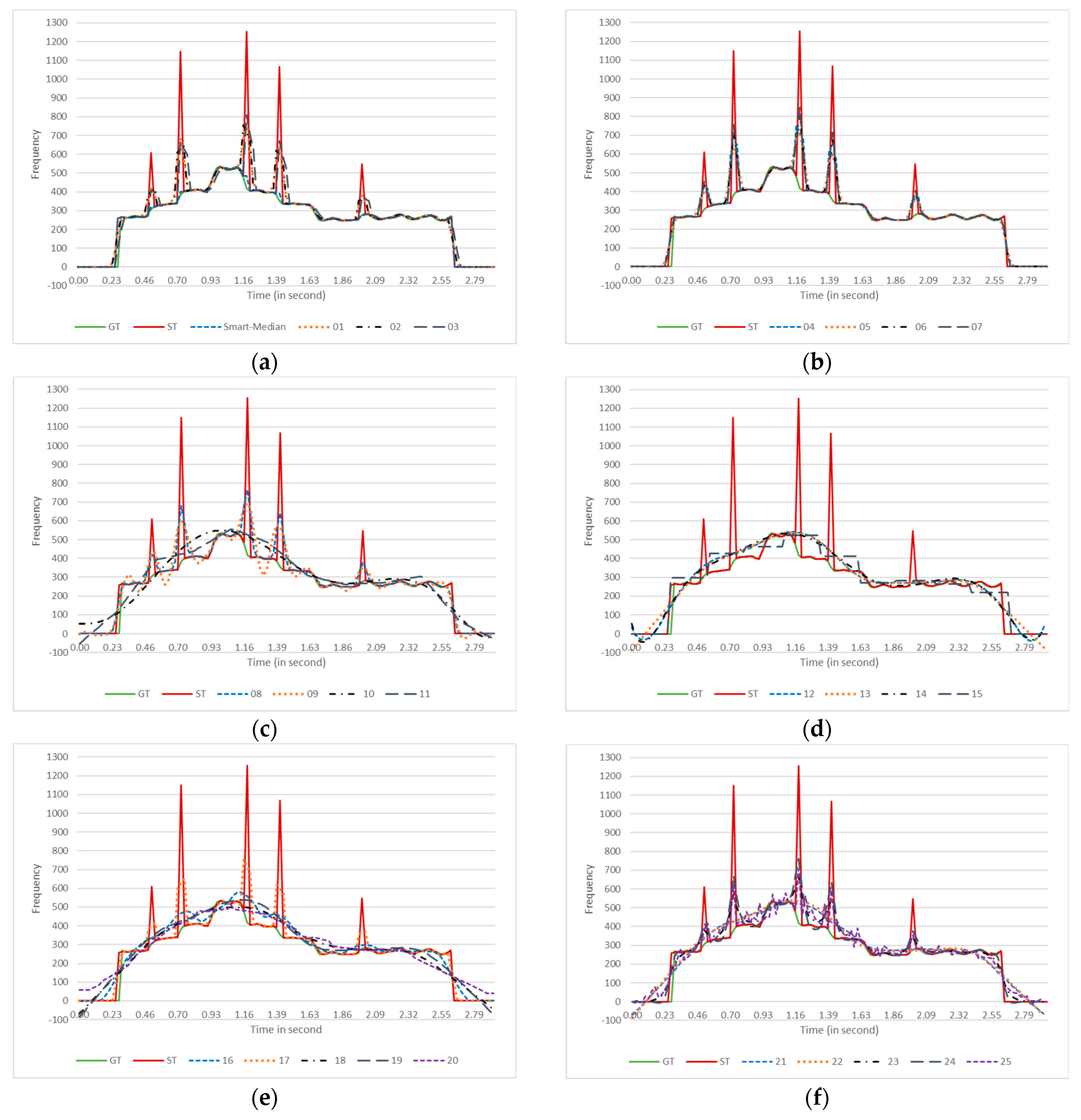
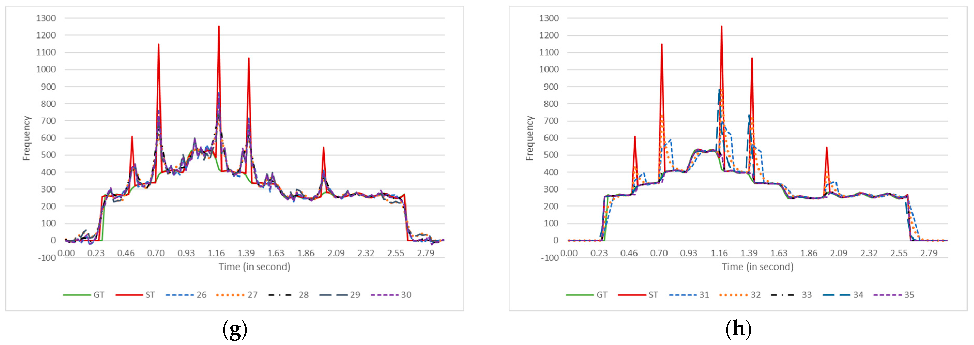
5. Results

This section provides the results of the comparisons between the Smart-Median algorithm and the other 35 contour smoothers mentioned in Section 3.3. Three groups of data were obtained for evaluation. These groups were 1—the ground truth pitch contour (GT), 2—the original estimated pitches (ES), and 3—the smoothed contour. The metrics explained in Section 3.5 were employed to compare these data groups. The data series were compared two by two, i.e., GT with ES, GT with SM, and ES with SM.

Table A4. Comparing pitch estimators and contour smoothers algorithms by ground truth based on the mean absolute error (MAE) metric. GT = Ground Truth, ES = Estimated pitch contour, SM = Smoothed contour.

Algorithm	Specacf			Schmitt			FComb			MComb			Yin			YinFFT			Praat			PYin (GT)
	GT-ES	GT-SM	ES-SM	GT-ES	GT-SM	ES-SM	GT-ES	GT-SM	ES-SM	GT-ES	GT-SM	ES-SM	GT-ES	GT-SM	ES-SM	GT-ES	GT-SM	ES-SM	GT-ES	GT-SM	ES-SM	GT-ES	GT-SM	ES-SM
00	256	123	208	68	61	26	123	42	108	46	32	28	588	114	543	61	26	39	14	14	0.7	0	1.2	1.2
01	256	233	112	68	63	20	123	122	56	46	47	15	588	581	291	61	60	35	14	14	0.2	0	3	3
02	256	236	128	68	64	21	123	122	59	46	47	15	588	584	316	61	60	37	14	14	0.2	0	2.7	2.7
03	256	234	118	68	62	26	123	122	62	46	47	20	588	583	302	61	58	40	14	13	1.2	0	5.5	5.5
04	256	236	128	68	64	21	123	122	59	46	47	15	588	584	316	61	60	37	14	14	0.2	0	2.7	2.7
05	256	232	124	68	63	23	123	122	63	46	48	17	588	582	325	61	60	40	14	14	0.3	0	3.4	3.4
06	256	235	104	68	64	18	123	122	51	46	47	13	588	582	266	61	60	32	14	14	0.2	0	2.5	2.5
07	256	237	96	68	64	16	123	122	44	46	47	11	588	584	237	61	60	28	14	14	0.1	0	2	2
08	256	233	113	68	64	20	123	122	56	46	47	15	588	582	291	61	60	35	14	14	0.2	0	2.9	2.9
09	256	244	147	68	69	30	123	137	83	46	54	24	588	743	545	61	77	59	14	14	0.5	0	5.6	5.6
10	256	226	208	68	77	72	123	138	146	46	72	64	588	628	624	61	87	100	14	43	38.2	0	44.3	44.3
11	256	227	184	68	68	55	123	131	122	46	59	46	588	626	567	61	74	81	14	21	13.4	0	23.6	23.6
12	256	227	181	68	68	52	123	131	120	46	58	44	588	648	579	61	74	79	14	21	13.1	0	21.5	21.5
13	256	227	190	68	71	59	123	133	128	46	63	52	588	613	580	61	77	87	14	21	13.9	0	28.7	28.7
14	256	226	186	68	68	56	123	132	127	46	60	48	588	660	619	61	77	84	14	22	14.3	0	24.2	24.2
15	256	227	189	68	72	61	123	132	126	46	64	53	588	580	535	61	76	84	14	25	17.5	0	31.2	31.2
16	256	223	168	68	64	44	123	123	104	46	53	37	588	580	478	61	66	67	14	18	10	0	16.9	16.9
17	256	236	128	68	64	21	123	122	59	46	47	15	588	584	316	61	60	37	14	14	0.2	0	2.7	2.7
18	256	214	195	68	69	64	123	126	132	46	62	55	588	571	569	61	74	88	14	23	15.8	0	31.1	31.1
19	256	227	190	68	71	59	123	133	128	46	63	52	588	613	580	61	77	87	14	21	13.9	0	28.7	28.7
20	256	227	190	68	71	59	123	133	128	46	63	52	588	613	580	61	77	87	14	21	13.9	0	28.7	28.7
21	264	227	189	68	66	56	128	129	125	47	58	47	591	577	519	62	72	83	14	21	13.7	0	24.5	24.5
22	256	227	190	68	71	59	123	133	128	46	63	52	588	613	580	61	77	87	14	21	13.9	0	28.7	28.7
23	256	225	136	68	62	32	123	121	78	46	50	26	588	576	381	61	62	52	14	14	0.8	0	7.3	7.3
24	256	234	116	68	64	22	123	124	60	46	48	17	588	599	322	61	62	39	14	14	0.2	0	3.2	3.2
25	256	231	137	68	65	38	123	129	87	46	54	32	588	665	483	61	73	61	14	14	1.7	0	11.9	11.9
26	256	245	102	68	66	20	123	132	57	46	50	16	588	703	380	61	72	41	14	14	0.3	0	3.6	3.6
27	256	229	133	68	64	30	123	125	76	46	51	25	588	623	410	61	67	51	14	14	1.5	0	9	9
28	256	235	122	68	65	23	123	126	65	46	49	18	588	634	373	61	66	43	14	14	0.3	0	4.5	4.5
29	256	236	114	68	65	27	123	128	67	46	52	23	588	656	386	61	71	47	14	14	1.5	0	9	9
30	256	244	105	68	66	21	123	131	59	46	50	17	588	694	380	61	72	41	14	14	0.4	0	4.4	4.4
31	261	235	153	69	62	39	126	125	88	47	51	30	600	592	411	62	61	57	14	13	2	0	9.4	9.4
32	256	232	97	68	61	23	123	121	54	46	47	18	588	580	258	61	58	35	14	13	1.3	0	5.7	5.7
33	256	228	96	68	63	11	123	108	33	46	45	6	588	417	201	61	48	20	14	14	0	0	0.3	0.3
34	256	226	122	68	62	20	123	113	54	46	46	13	588	510	292	61	54	35	14	14	0.1	0	1.9	1.9
35	256	234	102	68	64	9	123	107	36	46	44	5	588	410	240	61	46	19	14	14	0	0	0	0

,

Table A5. Comparing pitch estimators and contour-smoother algorithms by ground truth based on the R-squared (R²) metric. GT = Ground Truth, ES = Estimated pitch contour, SM = Smoothed contour.

Algorithm	Specacf			Schmitt			FComb			MComb			Yin			YinFFT			Praat			PYin (GT)
	GT-ES	GT-SM	ES-SM	GT-ES	GT-SM	ES-SM	GT-ES	GT-SM	ES-SM	GT-ES	GT-SM	ES-SM	GT-ES	GT-SM	ES-SM	GT-ES	GT-SM	ES-SM	GT-ES	GT-SM	ES-SM	GT-ES	GT-SM	ES-SM
00	−28	−3	0	−0.5	−0.3	0.7	−22	−1	0.3	−1	0.2	0.7	−1153	−3	−0.4	−22	1	0.7	0.8	0.84	1	1	0.97	0.97
01	−28	−20	0.8	−0.5	−0.2	1	−22	−17	0.8	−1	−0.9	1	−1153	−462	0.7	−22	−10	0.9	0.8	0.81	1	1	0.99	0.99
02	−28	−20	0.7	−0.5	−0.3	0.9	−22	−17	0.8	−1	−0.9	0.9	−1153	−516	0.6	−22	−11	0.9	0.8	0.81	1	1	0.99	0.99
03	−28	−20	0.7	−0.5	−0.3	0.9	−22	−17	0.8	−1	−0.9	0.9	−1153	−526	0.6	−22	−11	0.9	0.8	0.81	1	1	0.98	0.98
04	−28	−20	0.7	−0.5	−0.3	0.9	−22	−17	0.8	−1	−0.9	0.9	−1153	−517	0.6	−22	−11	0.9	0.8	0.81	1	1	0.99	0.99
05	−28	−19	0.7	−0.5	−0.2	0.9	−22	−16	0.8	−1	−0.8	0.9	−1153	−428	0.6	−22	−10	0.9	0.8	0.81	1	1	0.99	0.99
06	−28	−20	0.8	−0.5	−0.3	1	−22	−17	0.9	−1	−0.9	1	−1153	−501	0.7	−22	−11	0.9	0.8	0.81	1	1	0.99	0.99
07	−28	−21	0.8	−0.5	−0.3	1	−22	−18	0.9	−1	−1	1	−1153	−561	0.8	−22	−12	0.9	0.8	0.81	1	1	1	1
08	−28	−20	0.7	−0.5	−0.3	1	−22	−17	0.8	−1	−0.9	1	−1153	−469	0.7	−22	−11	0.9	0.8	0.81	1	1	0.99	0.99
09	−28	−20	0.6	−0.5	−0.3	0.9	−22	−17	0.8	−1	−0.9	0.9	−1153	−490	0.5	−22	−11	0.8	0.8	0.81	1	1	0.99	0.99
10	−28	−15	0.4	−0.5	0	0.6	−22	−10	0.5	−1	−0.4	0.7	−1153	−191	0.2	−22	−5	0.6	0.8	0.6	0.7	1	0.79	0.79
11	−28	−17	0.5	−0.5	0	0.8	−22	−13	0.6	−1	−0.5	0.8	−1153	−239	0.3	−22	−6	0.7	0.8	0.8	1	1	0.93	0.93
12	−28	−17	0.5	−0.5	0	0.8	−22	−13	0.6	−1	−0.5	0.8	−1153	−267	0.4	−22	−7	0.7	0.8	0.8	1	1	0.94	0.94
13	−28	−16	0.4	−0.5	0	0.7	−22	−12	0.6	−1	−0.5	0.8	−1153	−204	0.3	−22	−6	0.7	0.8	0.8	1	1	0.9	0.9
14	−28	−16	0.4	−0.5	0	0.8	−22	−12	0.6	−1	−0.5	0.8	−1153	−245	0.3	−22	−6	0.7	0.8	0.79	1	1	0.93	0.93
15	−28	−16	0.4	−0.5	0	0.7	−22	−12	0.5	−1	−0.5	0.7	−1153	−238	0.3	−22	−6	0.6	0.8	0.77	0.9	1	0.85	0.85
16	−28	−17	0.5	−0.5	0	0.8	−22	−13	0.6	−1	−0.5	0.8	−1153	−259	0.4	−22	−6	0.7	0.8	0.81	1	1	0.95	0.95
17	−28	−20	0.7	−0.5	−0.3	0.9	−22	−17	0.8	−1	−0.9	0.9	−1153	−517	0.6	−22	−11	0.9	0.8	0.81	1	1	0.99	0.99
18	−28	−15	0.4	−0.5	0.2	0.7	−22	−10	0.5	−1	−0.3	0.7	−1153	−155	0.3	−22	−4	0.6	0.8	0.8	0.9	1	0.89	0.89
19	−28	−16	0.4	−0.5	0	0.7	−22	−12	0.6	−1	−0.5	0.8	−1153	−204	0.3	−22	−6	0.7	0.8	0.8	1	1	0.9	0.9
20	−28	−16	0.4	−0.5	0	0.7	−22	−12	0.6	−1	−0.5	0.8	−1153	−204	0.3	−22	−6	0.7	0.8	0.8	1	1	0.9	0.9
21	−30	−17	0.4	−0.6	0.1	0.7	−24	−12	0.5	−1	−0.4	0.8	−1208	−194	0.3	−23	−5	0.7	0.8	0.8	1	1	0.92	0.92
22	−28	−16	0.4	−0.5	0	0.7	−22	−12	0.6	−1	−0.5	0.8	−1153	−204	0.3	−22	−6	0.7	0.8	0.8	1	1	0.9	0.9
23	−28	−18	0.7	−0.5	−0.1	0.9	−22	−14	0.8	−1	−0.6	0.9	−1153	−288	0.6	−22	−7	0.8	0.8	0.81	1	1	0.98	0.98
24	−28	−20	0.7	−0.5	−0.3	0.9	−22	−17	0.8	−1	−0.9	1	−1153	−457	0.7	−22	−10	0.9	0.8	0.81	1	1	0.99	0.99
25	−28	−18	0.7	−0.5	0	0.9	−22	−14	0.8	−1	−0.6	0.9	−1153	−349	0.7	−22	−8	0.8	0.8	0.81	1	1	0.98	0.98
26	−28	−21	0.8	−0.5	−0.3	1	−22	−17	0.9	−1	−0.9	1	−1153	−584	0.8	−22	−13	0.9	0.8	0.81	1	1	1	1
27	−28	−18	0.7	−0.5	−0.1	0.9	−22	−14	0.8	−1	−0.6	0.9	−1153	−353	0.6	−22	−9	0.9	0.8	0.81	1	1	0.98	0.98
28	−28	−19	0.7	−0.5	−0.2	0.9	−22	−16	0.8	−1	−0.8	0.9	−1153	−449	0.7	−22	−10	0.9	0.8	0.81	1	1	0.99	0.99
29	−28	−19	0.8	−0.5	−0.1	0.9	−22	−15	0.9	−1	−0.7	0.9	−1153	−468	0.8	−22	−11	0.9	0.8	0.81	1	1	0.99	0.99
30	−28	−21	0.8	−0.5	−0.3	1	−22	−17	0.9	−1	−0.9	1	−1153	−563	0.8	−22	−13	0.9	0.8	0.81	1	1	0.99	0.99
31	−31	−22	0.6	−0.7	−0.3	0.8	−25	−18	0.7	−2	−1	0.8	−1308	−478	0.5	−25	−11	0.8	0.8	0.81	1	1	0.96	0.96
32	−28	−20	0.8	−0.5	−0.2	0.9	−22	−17	0.9	−1	−0.8	0.9	−1153	−501	0.8	−22	−11	0.9	0.8	0.81	1	1	0.99	0.99
33	−28	−23	0.6	−0.5	−0.4	1	−22	−19	0.8	−1	−1.1	1	−1153	−266	0.4	−22	−12	0.8	0.8	0.81	1	1	1	1
34	−28	−20	0.6	−0.5	−0.3	0.9	−22	−17	0.7	−1	−0.9	0.9	−1153	−389	0.5	−22	−9	0.8	0.8	0.81	1	1	0.99	0.99
35	−28	−22	0.5	−0.5	−0.4	0.9	−22	−20	0.7	−1	−1.1	0.9	−1153	−376	0.4	−22	−11	0.8	0.8	0.81	1	1	1	1

,

Table A6. Comparing pitch estimators and contour-smoother algorithms by ground truth based on the Root-Mean-Square Error (RMSE) metric. GT = Ground Truth, ES = Estimated pitch contour, SM = Smoothed contour.

Algorithm	Specacf			Schmitt			FComb			MComb			Yin			YinFFT			Praat			PYin (GT)
	GT-ES	GT-SM	ES-SM	GT-ES	GT-SM	ES-SM	GT-ES	GT-SM	ES-SM	GT-ES	GT-SM	ES-SM	GT-ES	GT-SM	ES-SM	GT-ES	GT-SM	ES-SM	GT-ES	GT-SM	ES-SM	GT-ES	GT-SM	ES-SM
00	394	161	370	111	96	73	258	79	240	96	66	62	2086	153	2077	194	58	159	21	21	3.1	0	4.5	4.5
01	394	307	188	111	97	36	258	206	112	96	84	32	2086	1342	1210	194	137	102	21	21	1.1	0	9.5	9.5
02	394	315	220	111	99	40	258	211	127	96	86	36	2086	1417	1405	194	143	117	21	21	1.1	0	10.2	10.2
03	394	315	201	111	96	48	258	210	131	96	84	43	2086	1427	1306	194	141	115	21	20	2.4	0	14.8	14.8
04	394	315	220	111	99	40	258	211	127	96	86	36	2086	1417	1405	194	143	117	21	21	1.1	0	10.2	10.2
05	394	302	207	111	96	40	258	202	124	96	84	36	2086	1291	1332	194	134	113	21	21	1.2	0	10.7	10.7
06	394	312	176	111	99	33	258	210	104	96	85	30	2086	1396	1130	194	142	95	21	21	1	0	8.6	8.6
07	394	321	165	111	101	30	258	216	95	96	87	27	2086	1475	1054	194	148	88	21	21	0.9	0	7.7	7.7
08	394	308	190	111	98	36	258	206	113	96	85	32	2086	1351	1221	194	138	103	21	21	1.1	0	9.5	9.5
09	394	311	228	111	101	47	258	211	141	96	87	42	2086	1373	1484	194	141	127	21	21	1.3	0	12.4	12.4
10	394	256	300	111	96	97	258	167	218	96	91	90	2086	818	1839	194	117	185	21	53	46.8	0	60.6	60.6
11	394	265	277	111	88	77	258	172	192	96	80	70	2086	936	1768	194	110	165	21	27	17.5	0	34.8	34.8
12	394	266	274	111	88	75	258	173	190	96	79	67	2086	990	1741	194	113	161	21	27	17.1	0	31.5	31.5
13	394	263	281	111	90	81	258	172	198	96	82	74	2086	851	1816	194	109	171	21	27	17.9	0	40.6	40.6
14	394	260	280	111	87	79	258	167	196	96	79	70	2086	940	1770	194	110	165	21	28	18.6	0	34.3	34.3
15	394	266	285	111	95	87	258	176	202	96	88	81	2086	906	1800	194	119	175	21	33	23.8	0	49.1	49.1
16	394	266	263	111	87	67	258	172	176	96	77	60	2086	964	1685	194	110	152	21	24	13.4	0	28	28
17	394	315	220	111	99	40	258	211	127	96	86	36	2086	1417	1405	194	143	117	21	21	1.1	0	10.2	10.2
18	394	243	288	111	86	86	258	155	205	96	80	79	2086	772	1836	194	102	175	21	29	20.5	0	44.2	44.2
19	394	263	281	111	90	81	258	172	198	96	82	74	2086	851	1816	194	109	171	21	27	17.9	0	40.6	40.6
20	394	263	281	111	90	81	258	172	198	96	82	74	2086	851	1816	194	109	171	21	27	17.9	0	40.6	40.6
21	403	259	283	110	84	78	265	164	200	96	78	72	2038	823	1739	199	105	172	21	27	17.8	0	36.7	36.7
22	394	263	281	111	90	81	258	172	198	96	82	74	2086	851	1816	194	109	171	21	27	17.9	0	40.6	40.6
23	394	279	216	111	89	49	258	183	138	96	78	44	2086	1071	1404	194	117	123	21	21	1.9	0	14.6	14.6
24	394	306	192	111	98	38	258	206	116	96	85	34	2086	1331	1235	194	137	105	21	21	1.2	0	9.9	9.9
25	394	284	203	111	88	53	258	183	137	96	78	48	2086	1199	1278	194	126	116	21	21	2.9	0	18.5	18.5
26	394	322	153	111	100	31	258	215	94	96	87	27	2086	1511	954	194	150	81	21	21	1	0	8	8
27	394	287	207	111	92	45	258	190	129	96	81	41	2086	1197	1334	194	127	116	21	21	2.7	0	15.5	15.5
28	394	304	197	111	97	39	258	204	119	96	84	35	2086	1332	1268	194	137	107	21	21	1.2	0	10.5	10.5
29	394	303	169	111	93	39	258	198	108	96	82	36	2086	1376	1052	194	140	93	21	21	2.5	0	14.3	14.3
30	394	319	158	111	99	32	258	212	96	96	86	28	2086	1495	978	194	149	84	21	21	1.1	0	8.7	8.7
31	397	303	247	112	93	65	261	200	168	97	82	59	2109	1294	1613	196	130	147	21	19	3.9	0	22	22
32	394	311	162	111	93	40	258	205	106	96	81	36	2086	1400	1044	194	138	93	21	20	2.5	0	13.4	13.4
33	394	319	250	111	103	33	258	219	127	96	90	26	2086	790	1591	194	124	123	21	21	0.6	0	1.5	1.5
34	394	305	249	111	97	46	258	206	144	96	86	39	2086	1143	1566	194	132	131	21	21	0.9	0	9.1	9.1
35	394	317	277	111	105	43	258	220	142	96	90	28	2086	729	1779	194	117	123	21	21	0.6	0	0	0

,

Table A7. Comparing pitch estimators and contour-smoother algorithms by ground truth based on the F0 Frame Error (FFE) metric. GT = Ground Truth, ES = Estimated pitch contour, SM = Smoothed contour.

Algorithm	Specacf			Schmitt			FComb			MComb			Yin			YinFFT			Praat			PYin (GT)
	GT-ES	GT-SM	ES-SM	GT-ES	GT-SM	ES-SM	GT-ES	GT-SM	ES-SM	GT-ES	GT-SM	ES-SM	GT-ES	GT-SM	ES-SM	GT-ES	GT-SM	ES-SM	GT-ES	GT-SM	ES-SM	GT-ES	GT-SM	ES-SM
00	40	48	61	67	69	89	77	82	84	84	87	92	45	52	63	88	90	97	95	95.1	99.8	100	99.8	99.8
01	40	33	60	67	64	86	77	63	72	84	77	86	45	36	77	88	81	85	95	95.1	100	100	95.7	95.7
02	40	35	61	67	66	90	77	66	77	84	79	91	45	39	83	88	84	91	95	95.1	100	100	98.3	98.3
03	40	36	64	67	67	87	77	67	78	84	80	91	45	40	83	88	84	91	95	95.1	100	100	98.3	98.3
04	40	35	61	67	66	90	77	66	77	84	79	91	45	39	83	88	84	91	95	95.1	100	100	98.3	98.3
05	40	34	61	67	65	88	77	64	74	84	78	88	45	37	79	88	82	88	95	95.1	100	100	97.4	97.4
06	40	35	65	67	65	89	77	65	76	84	79	89	45	38	81	88	82	88	95	95.1	100	100	97.4	97.4
07	40	36	69	67	66	92	77	66	80	84	79	92	45	39	85	88	84	91	95	95.1	100	100	98.3	98.3
08	40	34	63	67	65	89	77	65	75	84	78	89	45	38	80	88	82	88	95	95.1	100	100	97.4	97.4
09	40	20	41	67	52	70	77	47	54	84	65	73	45	15	43	88	64	68	95	95.1	100	100	84.6	84.6
10	40	21	32	67	46	51	77	41	42	84	54	58	45	13	33	88	55	57	95	83.3	86.9	100	72	72
11	40	21	36	67	49	58	77	44	46	84	60	65	45	17	44	88	61	63	95	95.2	99.6	100	80.1	80.1
12	40	21	36	67	49	59	77	44	47	84	61	66	45	17	42	88	62	64	95	95.2	99.6	100	81.3	81.3
13	40	21	35	67	47	56	77	42	44	84	57	62	45	16	41	88	58	60	95	95.2	99.6	100	76.8	76.8
14	40	20	35	67	48	58	77	43	45	84	60	65	45	13	35	88	60	62	95	95.2	99.5	100	80.6	80.6
15	40	27	42	67	55	64	77	51	54	84	65	70	45	26	56	88	68	70	95	94.5	98.8	100	83.2	83.2
16	40	27	44	67	56	68	77	52	55	84	67	73	45	26	58	88	70	72	95	95.2	99.7	100	86	86
17	40	35	61	67	66	90	77	66	77	84	79	91	45	39	83	88	84	91	95	95.1	100	100	98.3	98.3
18	40	22	34	67	47	54	77	43	44	84	56	61	45	17	41	88	58	60	95	95.3	99.4	100	75.6	75.6
19	40	21	35	67	47	56	77	42	44	84	57	62	45	16	41	88	58	60	95	95.2	99.6	100	76.8	76.8
20	40	21	35	67	47	56	77	42	44	84	57	62	45	16	41	88	58	60	95	95.2	99.6	100	76.8	76.8
21	38	21	36	66	50	58	76	45	47	83	60	65	43	18	47	88	62	64	95	95.3	99.6	100	79.8	79.8
22	40	21	35	67	47	56	77	42	44	84	57	62	45	16	41	88	58	60	95	95.2	99.6	100	76.8	76.8
23	40	22	45	67	52	70	77	50	56	84	64	72	45	22	59	88	67	71	95	95.1	100	100	85.1	85.1
24	40	23	49	67	53	74	77	53	61	84	67	75	45	25	64	88	70	74	95	95.1	100	100	86.7	86.7
25	40	21	43	67	51	67	77	47	53	84	63	70	45	16	43	88	63	66	95	95.1	99.9	100	83.3	83.3
26	40	21	51	67	53	76	77	51	61	84	66	76	45	19	54	88	66	70	95	95.1	100	100	84.8	84.8
27	40	22	45	67	52	71	77	50	57	84	65	74	45	21	56	88	67	71	95	95.1	99.9	100	84.7	84.7
28	40	22	47	67	53	73	77	51	59	84	66	74	45	22	59	88	68	72	95	95.1	100	100	84.6	84.6
29	40	21	49	67	52	74	77	50	59	84	66	74	45	19	52	88	66	70	95	95.1	99.9	100	84.8	84.8
30	40	21	50	67	53	75	77	50	60	84	66	76	45	19	53	88	66	71	95	95.1	100	100	84.9	84.9
31	39	34	57	66	66	80	76	64	72	83	78	87	44	37	76	88	82	87	95	95.2	99.9	100	97.2	97.2
32	40	30	60	67	60	80	77	61	70	84	74	82	45	32	72	88	77	82	95	95.1	100	100	92.8	92.8
33	40	42	80	67	69	95	77	79	94	84	84	98	45	45	95	88	89	99	95	95.1	100	100	100	100
34	40	34	61	67	63	81	77	68	76	84	77	85	45	36	78	88	81	85	95	95.1	100	100	94.7	94.7
35	40	42	82	67	69	96	77	80	94	84	84	98	45	45	95	88	89	99	95	95.1	100	100	100	100

and

Table A8. Comparing the mean of pitch estimators and contour-smoother algorithms by ground truth based on the four metrics. GT = Ground Truth, ES = Estimated pitch contour, SM = Smoothed contour.

Algorithm	MAE			R2			RMSE			FFE
	GT-ES	GT-SM	ES-SM	GT-ES	GT-SM	ES-SM	GT-ES	GT-SM	ES-SM	GT-ES	GT-SM	ES-SM
00	165	59	136	−175	−1	0.4	451	91	426	71	75	84
01	165	160	76	−175	−73	0.9	451	313	240	71	64	81
02	165	161	82	−175	−81	0.8	451	327	278	71	66	85
03	165	160	81	−175	−82	0.8	451	327	264	71	67	85
04	165	161	82	−175	−81	0.8	451	327	278	71	66	85
05	165	160	85	−175	−68	0.8	451	304	265	71	65	82
06	165	161	69	−175	−79	0.9	451	324	224	71	66	84
07	165	161	62	−175	−87	0.9	451	338	209	71	66	87
08	165	160	76	−175	−74	0.9	451	315	242	71	65	83
09	165	191	127	−175	−77	0.8	451	321	296	71	51	64
10	165	181	179	−175	−32	0.5	451	228	397	71	45	51
11	165	172	153	−175	−39	0.7	451	240	367	71	50	59
12	165	175	153	−175	−43	0.7	451	248	361	71	50	59
13	165	172	158	−175	−34	0.6	451	228	377	71	48	57
14	165	178	162	−175	−40	0.6	451	239	368	71	49	57
15	165	168	152	−175	−39	0.6	451	241	379	71	55	65
16	165	161	130	−175	−42	0.7	451	243	345	71	56	67
17	165	161	82	−175	−81	0.8	451	327	278	71	66	85
18	165	163	160	−175	−26	0.6	451	210	384	71	48	56
19	165	172	158	−175	−34	0.6	451	228	377	71	48	57
20	165	172	158	−175	−34	0.6	451	228	377	71	48	57
21	168	164	147	−184	−32	0.6	448	220	366	70	50	60
22	165	172	158	−175	−34	0.6	451	228	377	71	48	57
23	165	159	101	−175	−47	0.8	451	262	282	71	53	67
24	165	164	82	−175	−72	0.9	451	312	246	71	55	71
25	165	176	120	−175	−55	0.8	451	283	262	71	51	63
26	165	183	88	−175	−91	0.9	451	344	192	71	53	70
27	165	168	104	−175	−56	0.8	451	285	268	71	53	68
28	165	170	92	−175	−71	0.9	451	311	252	71	54	69
29	165	175	95	−175	−73	0.9	451	316	214	71	53	68
30	165	182	89	−175	−88	0.9	451	340	197	71	53	69
31	168	163	111	−199	−76	0.7	456	303	329	70	65	80
32	165	159	70	−175	−78	0.9	451	321	212	71	61	78
33	165	132	52	−175	−46	0.8	451	238	307	71	72	94
34	165	146	76	−175	−62	0.8	451	284	311	71	65	81
35	165	131	59	−175	−61	0.7	451	228	342	71	72	95

show the accuracy of each of the pitch detector algorithms, and the accuracy of contour-smoother algorithms applied to the estimated pitch contours to bring them closer to the ground truth pitch contour. The GT–ES columns show the initial difference between ground truth and the original estimated pitch contour. Next, the differences between ground truth and the smoothed contours are shown in the GT–MS columns. Finally, the results of comparing the initially estimated pitch contour and the smoothed pitch contour are provided in the ES–SM columns. The metrics comparing GT and SM are more important than those comparing GT–ES and ES–SM, because the values of GT–SM illustrate the resulting improvement supplied by each algorithm. For example, in the Specacf column in Table A7, the first row (smoother algorithm with code 00) shows that according to the FFE metric GT–ES = 40, GT–SM = 48, and ES–SM = 61. That is, 40 per cent of the pitches estimated by the Specacf algorithm were correct. Then, the smoother algorithm improved this to 48 per cent acceptable data. Finally, 61 per cent of the values in the estimated pitch and smoothed contour remained in the same range; i.e., the smoother algorithm significantly changed 39 per cent of the values.

According to Table A4, Table A5, Table A6 and Table A7, the Smart-Median was the best algorithm for all pitch contours estimated by Specacf, FComb, MComb, Yin, or YinFFT. However, the best accuracy for the pitch contours calculated by Praat was recorded by the contour smoother code 33 (standard median). However, there was no agreement between the metrics employed to select the best smoother of pitch contours generated by Schmitt or PYin.

Table A8 aggregates all the data in Table A4, Table A5, Table A6 and Table A7. It can be observed in Table A8 that all the metrics agree that the Smart-Median worked better than the other smoother algorithms.

Only the GT–SM column was considered to have found significant differences between the accuracy of the algorithms. All the algorithms in the range of the column average plus/minus standard deviation were considered to exhibit a similar accuracy. The algorithms with values outside this range were considered to be in the best or worst category, as shown in

Table 2. Dividing the contour smoother algorithms into three categories (best, normal, and worst) based on the standard deviation.

	Best Code (Value)	Normal		Worst Code (Value)
MAE	00 (58.71) 33 (131.85) 35 (131.3)	Avg = 162.56	Std = 21.25	09 (190.95)
		Min = 141.31	Max = 183.81
		All the other algorithms
R2	00 (−0.72) 10 (−31.59) 13 (−34.07) 18 (−26.9) 19 (−34.7) 20 (−34.07) 21 (−32.46) 22 (−34.07)	Avg = −58.01	Std = 21.98	02 (−80.79) 03 (−82.22) 04 (−80.81) 07 (−87.46) 17 (−80.81) 26 (−90.75) 30 (−87.66)
		Min = −79.99	Max = −36.03
		All the other algorithms
RMSE	00 (90.67) 18 (209.56) 21 (220.12)	Avg = 275.62	Std = 53.1	07 (338.41) 26 (343.63) 30 (339.93)
		Min = 222.52	Max = 328.72
		All the other algorithms
FFE	00 (74.73) 02 (66.21) 03 (66.87) 04 (66.22) 07 (66.48) 17 (66.22) 33 (71.87) 35 (71.99)	Avg = 57.59	Std = 8.35	10 (44.83) 13 (48.24) 14 (48.6) 18 (48.47) 19 (48.24) 20 (48.24) 22 (48.24)
		Min = 49.24	Max = 65.94
		All the other algorithms

. There were certain agreements and disagreements between the metrics employed to find the best and worst algorithms. For example, the smoother code 07 was in the worst category based on the metrics MAE and RMSE, but in the best category based on the FFE metric. These agreements and disagreements are discussed in Section 6.

An ANOVA test was used to check the accuracy of the smoother algorithms. For all the metrics, the p-value calculated for each smoother algorithm was 0. That means that the accuracy of all the smoother algorithms depended on errors that occurred in the pitch contours, i.e., the smoother algorithms did not work with the same accuracy when each pitch contour was affected by different sources of error.

6. Discussion

This section discusses several aspects of the results obtained in Section 5. Because this paper focuses on the Smart-Median method, the only considerations provided here are those relating to comparisons of the accuracy of Smart-Median with that of other smoother algorithms.

6.1. Comparing the Results of Each Metric

A higher R² value does not always mean a better fitting [44]. For example,

Table 3. Comparison of metrics in different series of predicted data.

	1st	2nd	3rd	4th	5th	R2 Score	RMSE	MAE	FFE
Ground Truth	98 (G2)	98 (G2)	110 (A2)	98 (G2)	98 (G2)	NA	NA	NA	NA
Predict 1	98.2 (G2)	98.2 (G2)	123.2 (B2)	98.2 (G2)	98.2 (G2)	−0.61	5.91	2.8	0.8
Predict 2	98 (G2)	98 (G2)	123 (B2)	98 (G2)	98 (G2)	−0.56	5.81	2.6	0.8
Predict 3	98 (G2)	110 (A2)	110 (A2)	110 (A2)	98 (G2)	−0.33	7.59	4.8	0.6
Predict 4	98.2 (G2)	98.2 (G2)	110.2 (A2)	98.2 (G2)	98.2 (G2)	0.999	0.2	0.2	1

shows the R-squared scores of three series of predicted data. According to the R-squared (R²) scores in Table 3, the order of the best prediction to the worst was 4, 3, 2, then 1. However, Predict 3 estimated two wrong notes, such that each was one tone above the corresponding ground truth notes (A2 instead of G2), while Predicts 1 and 2 each had only one wrong estimated note (B2 instead of A2). Therefore, musically, the third was the worst, but based on R-squared, it was the second-best. In addition, musically, Predict 1 and Predict 2 were similar, and the 0.2 Hz pitch frequency difference could easily have resulted from a different method of F0 tracking, but their R-squared scores were different. In conclusion, we cannot compare two series of smoothed pitches based only on R-squared.

According to the RMSE and MAE columns in Table 3, the best to worst series were 4, 2, 1, then 3. This order is better than that based on R-squared. However, musically, we need to consider the similarity of Predict 1 and Predict 2; based on the FFE column in Table 3, Predicts 1 and 2 both had the same value. As shown in Table 3, Predict 4 was the best according to all the metrics, and musically, it was also the best. Moreover, although Predicts 1 and 2 were musically similar (FFE metric), Predict 2 was more accurate than Predict 1 (R², RMSE, and MAE metrics).

To conclude, a single metric alone cannot provide a clear and accurate evaluation to compare pitch contours, but a firm conclusion can be reached by using all of them.

6.2. Comparing Moving Average, Median, Okada, Jlassi, and Smart-Median

The main weakness of the Median, Okada [19], and Jlassi [20] filters is that they only adjust noises with a duration of one point in the contour. In other words, if more than one consecutive wrongly estimated pitch occurs within a contour, these algorithms cannot smooth the errors. The following example illustrates the operation of the moving average, Median, Okada, Jlassi, and Smart-Median approaches on a data series.

As shown in

Table 4. An example to illustrate the weakness of the moving average, Median, Okada, and Jlassi algorithms as compared to the Smart-Median.

Input	100	102	2000	2000	100
Moving average(window size = 3)	734	1367.333	1366.667	1050	100
Median (window size = 3)	102	2000	2000	1050	100
Okada	100	102	2000	2000	100
Jlassi	100	102	2000	2000	100
Smart-Median	100	102	102	102	100

, the moving average and Median methods changed some of the correctly estimated values, i.e., the 102 value which was the second piece of input data. On the other hand, Okada’s and Jlassi’s approaches did not change any of the values, because they look for significant differences with immediately preceding and following points. However, the Smart-Median is mainly concerned with finding an acceptable jump by comparing the current and previous points. Because of this different approach to identification of errors, when the pitch contour was already almost smooth (contours estimated by Praat and PYin) there was no significant difference between the accuracy of these approaches (as seen by comparing rows 00, 33, 34, and 35 in Praat and PYin columns in Table A4, Table A5, Table A6 and Table A7). However, while the pitch contours estimated by the other pitch detection algorithms exhibited several errors, Smart-Median appears to have worked in a meaningful manner that outperformed all other methods (observable in Specacf, Schmitt, FComb, MComb, Yin, and YinFFT columns in Table A4, Table A5, Table A6 and Table A7).

Generally, according to Table A8, the accuracy of Smart-Median based on the four metrics was much better than all the other algorithms.

6.3. Accuracy of the Contour Smoother Algorithms

All the contour smoother algorithms provided strong results according to the R² and RMSE metrics (by comparing the GT–ES columns with GT–SM columns in Table A8). However, only the Smart-Median (00), Median (33), and Jlassi (35) approaches could change the pitch contour to ensure that more of the estimated F0 values were constrained to the range of 20% of the ground truth pitch contour (Table A4, Table A5, Table A6, Table A7 and Table A8). Therefore, although all the algorithms smoothed contour errors, many also altered the value of the corrected estimated pitches.

7. Conclusions

This paper has introduced a new pitch-contour-smoother targeted towards the singing voice in real-time environments. The proposed algorithm is based on the median filter and considers the features of fundamental frequencies in singing. The algorithm’s accuracy was compared with 35 other smoother techniques, and four metrics evaluated their results: R-Squared, Root-Mean-Square Error, Mean Absolute Error, and F0 Frame Error. The proposed Smart-Median algorithm achieved better results across all the metrics, in comparison to the other smoother algorithms. According to this study, a buffer delay of 35 to 70 milliseconds is required for the algorithm to smooth the contour appropriately.

Most of the general smoother algorithms did not show acceptable accuracy. A general observation is that in the ideal case, a smoother algorithm should be defined based on the essential features of the data in the contour and how that data is to be used after smoothing.

For future work, one short-term task is based on recognizing that the parameters of the Smart-Median can be set according to the specific properties of the sound input, such as those of particular musical instruments or their families, to improve accuracy in a targeted way. Another task considers that the Smart-Median finds the incorrect F0 based on its interval from the previous F0; this approach can be improved by considering a maximum noise duration. For example, if there is a considerable frequency interval between the previous F0 and the current one, or if several immediately subsequent F0s are near to the current F0, then we may not consider the large jump to be noise but rather a new musical articulation. This requires the introduction of an extra decision-making stage into the algorithm. In the longer term, further testing can be carried out on vocal material from a wide variety of genres and techniques. This would require the creation of new, specialist corpora, requiring considerable manual effort in both the gathering and labelling. This can be supported by machine learning. Such a dataset would also benefit the research field at large.

References

- Ferro, M.; Tamburini, F. Using Deep Neural Networks for Smoothing Pitch Profiles in Connected Speech. Ital. J. Comput. Linguist. 2019, 5, 33–48. [Google Scholar] [CrossRef]
- Zhao, X.; O’Shaughnessy, D.; Nguyen, M.Q. A Processing Method for Pitch Smoothing Based on Autocorrelation and Cepstral F0 Detection Approaches. In Proceedings of the 2007 International Symposium on Signals, Systems and Electronics, Montreal, QC, Canada, 30 July–2 August 2007; pp. 59–62. [Google Scholar] [CrossRef]
- So, Y.; Jia, J.; Cai, L. Analysis and Improvement of Auto-Correlation Pitch Extraction Algorithm Based on Candidate Set; Lecture Notes in Electrical Engineering; Springer: Berlin/Heidelberg, Germany, 2012; Volume 128, pp. 697–702. ISBN 9783642257919. [Google Scholar]
- Faghih, B.; Timoney, J. An Investigation into Several Pitch Detection Algorithms for Singing Phrases Analysis. In Proceedings of the 2019 30th Irish Signals and Systems Conference (ISSC), Maynooth, Ireland, 17–18 June 2019; pp. 1–5. [Google Scholar]
- Faghih, B.; Timoney, J. Real-Time Monophonic Singing Pitch Detection. 2022; preprint. [Google Scholar] [CrossRef]
- Luers, J.K.; Wenning, R.H. Polynomial Smoothing: Linear vs Cubic. Technometrics 1971, 13, 589. [Google Scholar] [CrossRef]
- Craven, P.; Wahba, G. Smoothing Noisy Data with Spline Functions. Numer. Math. 1978, 31, 377–403. [Google Scholar] [CrossRef]
- Hutchinson, M.F.; de Hoog, F.R. Smoothing Noisy Data with Spline Functions. Numer. Math. 1985, 47, 99–106. [Google Scholar] [CrossRef]
- Deng, G.; Cahill, L.W. An Adaptive Gaussian Filter for Noise Reduction and Edge Detection. In Proceedings of the 1993 IEEE Conference Record Nuclear Science Symposium and Medical Imaging Conference, San Francisco, CA, USA, 31 October–6 November 1993; pp. 1615–1619. [Google Scholar]
- Cleveland, W.S. Robust Locally Weighted Regression and Smoothing Scatterplots. J. Am. Stat. Assoc. 1979, 74, 829–836. [Google Scholar] [CrossRef]
- Cleveland, W.S. LOWESS: A Program for Smoothing Scatterplots by Robust Locally Weighted Regression. Am. Stat. 1981, 35, 54. [Google Scholar] [CrossRef]
- Wen, Q.; Zhang, Z.; Li, Y.; Sun, L. Fast RobustSTL: Efficient and Robust Seasonal-Trend Decomposition for Time Series with Complex Patterns. In Proceedings of the 26th ACM SIGKDD International Conference on Knowledge Discovery & Data Mining, Virtual Event, CA, USA, 6–10 July 2020; pp. 2203–2213. [Google Scholar]
- Sampaio, M.D.S. Contour Similarity Algorithms. MusMat-Braz. J. Music Math. 2018, 2, 58–78. [Google Scholar]
- Wu, Y.D. A New Similarity Measurement of Pitch Contour for Analyzing 20th- and 21st-Century Music: The Minimally Divergent Contour Network. Indiana Theory Rev. 2013, 31, 5–51. [Google Scholar]
- Lin, H.; Wu, H.-H.; Kao, Y.-T. Geometric Measures of Distance between Two Pitch Contour Sequences. J. Comput. 2008, 19, 55–66. [Google Scholar]
- Chatterjee, I.; Gupta, P.; Bera, P.; Sen, J. Pitch Tracking and Pitch Smoothing Methods-Based Statistical Approach to Explore Singers’ Melody of Voice on a Set of Songs of Tagore; Springer: Singapore, 2018; Volume 462, ISBN 9789811079009. [Google Scholar]
- Smith, S.W. Moving Average Filters. In The Scientist & Engineer’s Guide to Digital Signal Processing; California Technical Publishing: San Clemente, CA, USA, 1999; pp. 277–284. ISBN 0-9660176-7-6. [Google Scholar]
- Kasi, K.; Zahorian, S.A. Yet Another Algorithm for Pitch Tracking. In Proceedings of the IEEE International Conference on Acoustics Speech and Signal Processing, Orlando, FL, USA, 13–17 May 2002; Volume 1, pp. I-361–I-364. [Google Scholar]
- Okada, M.; Ishikawa, T.; Ikegaya, Y. A Computationally Efficient Filter for Reducing Shot Noise in Low S/N Data. PLoS ONE 2016, 11, e0157595. [Google Scholar] [CrossRef]
- Jlassi, W.; Bouzid, A.; Ellouze, N. A New Method for Pitch Smoothing. In Proceedings of the 2016 2nd International Conference on Advanced Technologies for Signal and Image Processing (ATSIP), Monastir, Tunisia, 21–23 March 2016; pp. 657–661. [Google Scholar]
- Liu, Q.; Wang, J.; Wang, M.; Jiang, P.; Yang, X.; Xu, J. A Pitch Smoothing Method for Mandarin Tone Recognition. Int. J. Signal Process. Image Process. Pattern Recognit. 2013, 6, 245–254. [Google Scholar]
- Plante, F.; Meyer, G.; Ainsworth, W.A. A Pitch Extraction Reference Database. In Proceedings of the Fourth European Conference on Speech Communication and Technology, Madrid, Spain, 18–21 September 1995; EUROSPEECH: Madrid, Spain, 1995. [Google Scholar]
- Gawlik, M.; Wiesław, W. Modern Pitch Detection Methods in Singing Voices Analyzes. In Proceedings of the Euronoise 2018, Crete, Greece, 27–31 May 2018; pp. 247–254. [Google Scholar]
- Mauch, M.; Dixon, S. PYIN: A Fundamental Frequency Estimator Using Probabilistic Threshold Distributions. In Proceedings of the 2014 IEEE International Conference on Acoustics, Speech and Signal Processing (ICASSP), Florence, Italy, 4–9 May 2014; pp. 659–663. [Google Scholar] [CrossRef]
- De Cheveigné, A.; Kawahara, H. YIN, a Fundamental Frequency Estimator for Speech and Music. J. Acoust. Soc. Am. 2002, 111, 1917–1930. [Google Scholar] [CrossRef] [PubMed]
- Aubio. Available online: https://aubio.org/ (accessed on 1 February 2022).
- Brossier, P.M. Automatic Annotation of Musical Audio for Interactive Applications. Ph.D. Thesis, Queen Mary University of London, London, UK, 2006. [Google Scholar]
- Boersma, P.; van Heuven, V. PRAAT, a System for Doing Phonetics by Computer. Glot. Int. 2001, 5, 341–347. [Google Scholar]
- Boersma, P. Accurate Short-Term Analysis of the Fundamental Frequency and the Harmonics-To-Noise Ratio of a Sampled Sound. In Proceedings of the Institute of Phonetic Sciences; University of Amsterdam: Amsterdam, The Netherlands, 1993; Volume 17, pp. 97–110. [Google Scholar]
- Buitinck, L.; Louppe, G.; Blondel, M.; Pedregosa, F.; Mueller, A.; Grisel, O.; Niculae, V.; Prettenhofer, P.; Gramfort, A.; Grobler, J.; et al. API Design for Machine Learning Software: Experiences from the Scikit-Learn Project. arXiv 2013, arXiv:1309.0238. [Google Scholar]
- Colin Cameron, A.; Windmeijer, F.A.G. An R-Squared Measure of Goodness of Fit for Some Common Nonlinear Regression Models. J. Econom. 1997, 77, 329–342. [Google Scholar] [CrossRef]
- Drugman, T.; Alwan, A. Joint Robust Voicing Detection and Pitch Estimation Based on Residual Harmonics. In Proceedings of the Annual Conference of the International Speech Communication Association, Florence, Italy, 27–31 August 2011. [Google Scholar] [CrossRef]
- Savitzky, A.; Golay, M.J.E. Smoothing and Differentiation of Data by Simplified Least Squares Procedures. Anal. Chem. 1964, 36, 1627–1639. [Google Scholar] [CrossRef]
- Dai, W.; Selesnick, I.; Rizzo, J.-R.; Rucker, J.; Hudson, T. A Nonlinear Generalization of the Savitzky-Golay Filter and the Quantitative Analysis of Saccades. J. Vis. 2017, 17, 10. [Google Scholar] [CrossRef]
- Schmid, M.; Rath, D.; Diebold, U. Why and How Savitzky–Golay Filters Should Be Replaced. ACS Meas. Sci. Au 2022, 2, 185–196. [Google Scholar] [CrossRef]
- Rej, R. NIST/SEMATECH e-Handbook of Statistical Methods; American Association for Clinical Chemistry: Washington, DC, USA, 2003. [Google Scholar]
- Braun, S. WINDOWS. In Encyclopedia of Vibration; Elsevier: Amsterdam, The Netherlands, 2001; Volume 2, pp. 1587–1595. [Google Scholar]
- Podder, P.; Zaman Khan, T.; Haque Khan, M.; Muktadir Rahman, M. Comparative Performance Analysis of Hamming, Hanning and Blackman Window. Int. J. Comput. Appl. 2014, 96, 1–7. [Google Scholar] [CrossRef]
- Orfanidis, S.J. Local Polynomial Filters. In Applied Optimum Signal Processing; McGraw-Hill Publishing Company: New York, NY, USA, 2018; pp. 119–163. [Google Scholar]
- Jones, W.M.P. Kernel Smoothing; Chapman & Hall: London, UK, 1995. [Google Scholar]
- Dagum, E.B. Time Series Modeling and Decomposition. Statistica 2010, 70, 433–457. [Google Scholar] [CrossRef]
- Welch, G.F. Kalman Filter. In Computer Vision; Springer International Publishing: Cham, Switzerland, 2021; pp. 1–3. ISBN 9789533070940. [Google Scholar]
- Kroher, N.; Gomez, E. Automatic Transcription of Flamenco Singing From Polyphonic Music Recordings. IEEE/ACM Trans. Audio Speech Lang. Process. 2016, 24, 901–913. [Google Scholar] [CrossRef][Green Version]
- Lewis-Beck, M.S.; Skalaban, A. The R-Squared: Some Straight Talk. Polit. Anal. 1990, 2, 153–171. [Google Scholar] [CrossRef]
- McFee, B.; Metsai, A.; McVicar, M.; Balke, S.; Thomé, C.; Raffel, C.; Zalkow, F.; Malek, A.; Dana; Lee, K.; et al. Librosa/Librosa: 0.9.1 2022. Available online: https://librosa.org/doc/latest/index.html (accessed on 5 February 2022).
- Virtanen, P.; Gommers, R.; Oliphant, T.E.; Haberland, M.; Reddy, T.; Cournapeau, D.; Burovski, E.; Peterson, P.; Weckesser, W.; Bright, J.; et al. SciPy 1.0: Fundamental Algorithms for Scientific Computing in Python. Nat. Methods 2020, 17, 261–272. [Google Scholar] [CrossRef] [PubMed]
- Reback, J.; McKinney, W.; Jbrockmendel; den Bossche, J.V.; Augspurger, T.; Cloud, P.; Gfyoung; Sinhrks; Klein, A.; Roeschke, M.; et al. Pandas-Dev/Pandas: Pandas 1.0.3; Zenodo: Genève, Switzerland, 2020. [Google Scholar] [CrossRef]
- Barupal, D.K.; Fiehn, O. Scikit-Learn: Machine Learning in Python. J. Mach. Learn. Res. 2011, 2, 2825–2830. [Google Scholar]