Article

Towards a Deep-Learning Approach for Prediction of Fractional Flow Reserve from Optical Coherence Tomography

by
Cosmin-Andrei Hatfaludi
1,2,*,
Irina-Andra Tache
1,3,
Costin Florian Ciușdel
1,2,
Andrei Puiu
1,2,
Diana Stoian
1,2,
Lucian Mihai Itu
1,2,
Lucian Calmac
4,5,
Nicoleta-Monica Popa-Fotea
4,5,
Vlad Bataila
4 and
Alexandru Scafa-Udriste
4,5
1
Advanta, Siemens SRL, 15 Noiembrie Bvd, 500097 Brasov, Romania
2
Automation and Information Technology, Transilvania University of Brasov, Mihai Viteazu nr. 5, 5000174 Brasov, Romania
3
Department of Automatic Control and Systems Engineering, University Politehnica of Bucharest, 014461 Bucharest, Romania
4
Department of Cardiology, Emergency Clinical Hospital, 8 Calea Floreasca, 014461 Bucharest, Romania
5
Department Cardio-Thoracic, University of Medicine and Pharmacy “Carol Davila”, 8 Eroii Sanitari, 050474 Bucharest, Romania
*
Author to whom correspondence should be addressed.
Appl. Sci. 2022, 12(14), 6964; https://doi.org/10.3390/app12146964
Submission received: 13 April 2022 / Revised: 4 July 2022 / Accepted: 8 July 2022 / Published: 9 July 2022
(This article belongs to the Special Issue Deep Neural Networks in Medical Imaging)

Abstract

:
Cardiovascular disease (CVD) is the number one cause of death worldwide, and coronary artery disease (CAD) is the most prevalent CVD, accounting for 42% of these deaths. In view of the limitations of the anatomical evaluation of CAD, Fractional Flow Reserve (FFR) has been introduced as a functional diagnostic index. Herein, we evaluate the feasibility of using deep neural networks (DNN) in an ensemble approach to predict the invasively measured FFR from raw anatomical information that is extracted from optical coherence tomography (OCT). We evaluate the performance of various DNN architectures under different formulations: regression, classification—standard, and few-shot learning (FSL) on a dataset containing 102 intermediate lesions from 80 patients. The FSL approach that is based on a convolutional neural network leads to slightly better results compared to the standard classification: the per-lesion accuracy, sensitivity, and specificity were 77.5%, 72.9%, and 81.5%, respectively. However, since the 95% confidence intervals overlap, the differences are statistically not significant. The main findings of this study can be summarized as follows: (1) Deep-learning (DL)-based FFR prediction from reduced-order raw anatomical data is feasible in intermediate coronary artery lesions; (2) DL-based FFR prediction provides superior diagnostic performance compared to baseline approaches that are based on minimal lumen diameter and percentage diameter stenosis; and (3) the FFR prediction performance increases quasi-linearly with the dataset size, indicating that a larger train dataset will likely lead to superior diagnostic performance.

1. Introduction

Cardiovascular disease (CVD) is the number one cause of death worldwide, and coronary artery disease (CAD) is the most prevalent CVD, accounting for 42% of these deaths. In CAD patients, plaque builds up in the coronary arteries and limits the blood flow to the myocardium, especially when the demand is increased (exercise, stress). In severe cases, this can lead to myocardial infarction, or even death.
X-ray coronary angiography (XA) represents the gold standard in CAD imaging [1]. Optical coherence tomography (OCT) is used in certain scenarios in conjunction with XA. OCT has the highest resolution among all invasive imaging modalities, allowing for a precise intra-vascular evaluation of stent apposition and expansion [2,3,4], thus, representing a paramount tool for PCI (percutaneous coronary intervention) optimization [5]. Nonetheless, its ability to assess the functional significance of a stenosis is not negligible [6].
The purely anatomical assessment of CAD, independent from the medical imaging modality, does not fully capture the functional significance of coronary stenoses. In view of the limitations of the anatomical evaluation of CAD, Fractional Flow Reserve (FFR) has been introduced as a functional index. FFR is defined as the ratio of flow in the stenosed branch at hyperemia—a condition of stress, with maximum coronary blood flow—to the hypothetical hyperemic flow in the same branch under healthy conditions. This can be shown to be closely approximated by the ratio of hyperemic cycle-averaged pressure distal to the stenosis to the cycle-averaged aortic pressure [7]. An FFR value ≤ 0.8 is considered to be positive, i.e., the patient requires invasive treatment, such as percutaneous coronary intervention (PCI-stenting) or coronary artery bypass graft (CABG). An FFR value > 0.8 is considered to be negative, i.e., typically only optimal medical therapy is prescribed. Several clinical trials have demonstrated the superiority of FFR-guided decision-making [8], which represents the current gold standard. However, although providing obvious advantages, studies indicate that the use of FFR is still relatively low due to the need to administer hyperemia-inducing drugs, additional costs, and the extended duration and invasive nature of the procedure [9]. Hence, computational approaches for FFR prediction have been introduced, relying either on computational fluid dynamics (CFD) or on artificial intelligence (AI).
Blood-flow computations, performed using CFD, when used in conjunction with patient-specific anatomical models that are extracted from medical images, have been proposed for diagnosis, risk stratification, and surgical planning [4]. Model-based assessment of coronary stenoses has been previously performed using such techniques in several clinical studies, based on anatomical models that are reconstructed from coronary computed tomography angiography (CCTA) [10,11,12,13], XA [14,15,16,17,18], or OCT [19,20,21,22]. Computed FFR has been the main quantity of interest in these studies, all of which showed that computed FFR has good diagnostic accuracy compared to invasively measured FFR. The CFD models consist of partial differential equations, which can be only numerically solved, leading to a large number of algebraic equations. Due to the time-consuming process that is employed for reconstructing the anatomical model, and the computationally intensive aspect of the CFD models [23,24], they are not used for intra-operative assessment and planning, where near real-time performance is required.
Alternatively, artificial intelligence-based solutions may be employed that are capable of providing results in real-time. To develop such solutions, a large database is required for the training phase, containing pairs of input-output data. The input data are represented by the anatomical information, while the output are invasive FFR [25]. Once the training phase has been finalized, the online usage provides results instantaneously. Such supervised machine learning (ML) algorithms are routinely employed in medical imaging applications, e.g., organ segmentation [26]. Moreover, machine learning models can also be employed to reproduce the behavior of non-linear computational models [27,28].
Recently, machine learning models for the prediction of FFR based on CCTA [29], XA [30], OCT [31], and intravascular ultrasound (IVUS) [32] have been introduced. All these approaches rely on the extraction of features describing the vascular geometry, specifically the arterial lumen, and, in some studies, also on patient features.
The goal of the present study is to evaluate the feasibility of using deep neural networks (DNN) to predict the invasively measured FFR from the radius of the coronary lumen that is extracted along the centerline of the coronary artery of interest. The starting point is represented by OCT images, the coronary lumen is then automatically extracted for each cross-section and subsequently processed to determine an equivalent radius value. The radius values are then arranged in a one-dimensional (1D) sequence, to be fed as input to the DNN. Our approach is in contrast to previous ML-based approaches for FFR prediction, since we use as input raw, reduced-order anatomical data instead of hand-crafted features. The second important aspect of the study is that we focus on intermediate lesions, for which the visual anatomical assessment of CAD based on XA does not allow for a clear clinical decision. As a result, the dataset contains a large number of lesions having an FFR value that is close to the cut-off of 0.8, making the prediction task more challenging.
Deep-learning (DL) is a class of machine learning algorithms that uses multiple layers to extract higher level features from the raw input [33]. The FFR prediction task can be formulated either as a regression problem (predict the exact value of FFR) or as a classification problem (predict the FFR class, e.g., binary classification: ≤0.8 or >0.8). There are several types of neural networks that are suitable for the FFR prediction, amongst others:
-
fully connected neural network, commonly referred to as artificial neural networks (ANNs). Potential disadvantages of ANNs are the large number of trainable parameters, which leads to the requirement of large training datasets, and the difficulty in capturing the inherent properties in 1D/2D/3D data structures
-
convolutional neural networks (CNNs). Compared to ANNs, CNNs can capture the inherent properties in 1D/2D/3D data structures, but still require relatively large training sets. Also, fixed size input data are required if the network is not fully convolutional.
-
recurrent neural networks (RNNs) [34]. RNNs have the advantage that a variable length input sequence can be processed, but they may be affected by vanishing and exploding gradient issues.
Few-shot learning (FSL) is a type of learning where the prediction is performed based on a limited number of samples [35]. In a study that was published by Yang et al., the models that were used for FSL were classified into four categories: multitask learning, embedding learning, learning with external memory, and generative modeling.
OCT images were previously used in a variety of DL-based applications: stent strut detection [36,37], stent strut segmentation [38,39,40], coronary calcification segmentation [41,42], atherosclerotic plaque characterization [43], and lumen segmentation [44]. Furthermore, DL-based approaches were employed also in studies addressing other types of optical signals [45,46].
Herein, we evaluate the performance of ANNs, CNNs, and RNNs in both regression and classification formulations. Additionally, we also consider the use of FSL, focusing specifically on prototypical networks [47], a subcategory of the embedding learning models, considered the state of the art for classification tasks. More details that are related to prototypical networks are included in Appendix A.1.

2. Materials and Methods

2.1. Data Set

2.1.1. Study Design

This was a single-center, retrospective study that was carried out at the Clinical Emergency Hospital, Bucharest, Romania. The study complied with the Declaration of Helsinki for investigation in human beings. The study protocol was approved by the local ethics committee and each patient signed an informed consent form before the enrolment in the study.

2.1.2. Study Population

Patients at least 18 years old, with stable angina, and an indication for diagnostic XA due to intermediate or high likelihood of obstructive coronary artery disease, were considered. Further inclusion criteria were: at least one lesion with 40% to 80% diameter stenosis by visual assessment, and invasive FFR measurement considered required by the operator for clinical decision-making. Patients were excluded if they were unable to provide informed consent, had significant arrhythmia (heart rate over 120 bpm), suspected acute coronary syndrome, atrial fibrillation, low systolic pressure (below 90 mmHg), contraindication to beta blockers, nitroglycerin or adenosine, a non-cardiac illness with a life expectancy of less than 2 years, pathological aortic valve, rest state angina, or myocardial infarct during the last 6 months. Additionally, aorto-ostial lesions were excluded from the study. A total of 80 patients were included in the study.

2.1.3. Procedure Protocol

Coronary angiography (Siemens Artis Zee, Forchheim, Germany) was performed after iso-centering in posterior-anterior and lateral planes, via a transradial (preferred) or transfemoral approach. In all cases, a 6 French diagnostic catheter was used after intracoronary injection of glyceryl trinitrate according to routine practice in the hospital, with manual contrast injection and cine acquisition at a frame rate of 15 frames/second. OCT imaging was performed using a frequency-domain OCT systems (St. Jude Medical/Abbott, St. Paul, MN, USA). The fiber probe was pulled back at a constant speed and cross-sectional images were generated with a spacing of 0.2 mm.
The acquisition of physiological data for FFR calculation was performed according to conventional practice [48] with a commercially available FFR measurement system (PressureWire Aeris; St. Jude Medical, Minneapolis, MN, USA). The 0.014 coronary wire with a pressure tip was advanced until the pressure sensor passed the orifice of the guiding catheter. Transcatheter aortic and intracoronary pressure tracings were equalized. Subsequently, the guidewire was advanced into the respective coronary artery until the pressure sensor passed the index lesion. Hyperemia was induced by the administration of adenosine either intravenously at a constant rate of 140 μg/kg/min, or as an intracoronary bolus (100 μg for the right and 200 μg for the left coronary artery); the pressure recording was started, and the FFR was determined. A total of 102 coronary lesions in 80 patients underwent FFR analysis. This invasively measured FFR represents the ground truth that is used during the training of the deep neural networks, as described in the following.

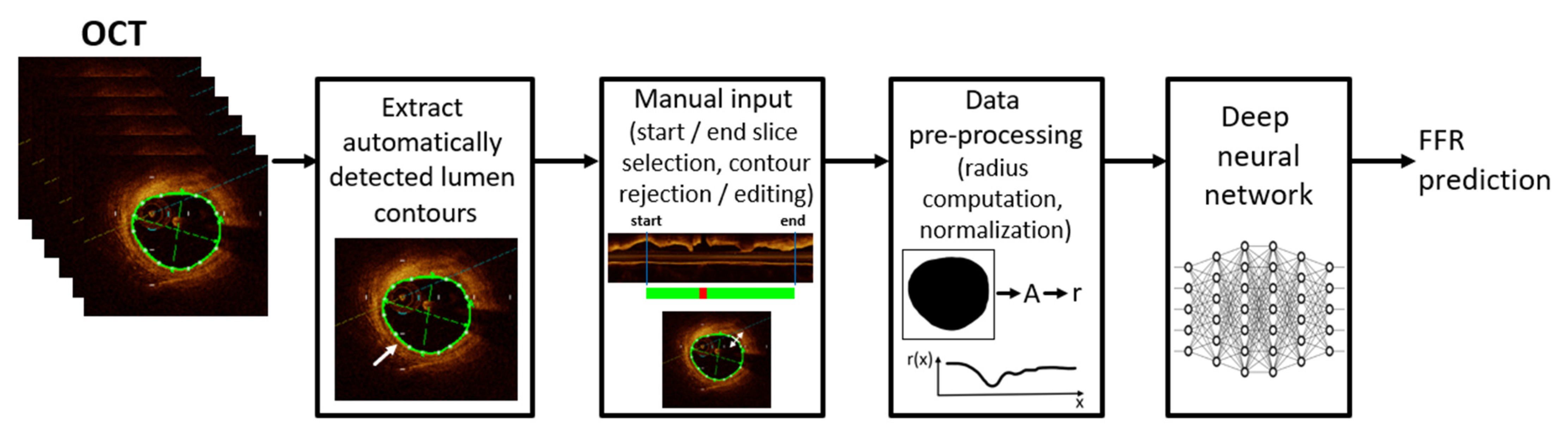
2.2. Data Pre-Processing

The OCT data were exported from the OCT workstation available onsite. All OCT slices are RGB images, and the exported data contains the automatically detected coronary lumen, which is overlaid on the image and depicted in green. The spacing between the slices is 0.2 mm, and the number of slices per acquisition is constant at 376. Figure 1 displays the data pre-processing workflow starting from the exported OCT images with automatically detected lumen contour. First, the contours are automatically extracted by processing the green channel as follows: a threshold representing 90% of the maximum intensity value is used to create a binary image, and all the contours are extracted [49]. We then retain the contour which surrounds the center of the image: if there are multiple such contours, we pick the one with the largest area. Next, we use an in-house developed application to collect manual input that is provided by the clinical expert:
-
selection of the proximal start and distal end slice, which define the coronary artery region of interest. Slices representing the catheter are excluded, alongside other slices with sub-optimal image quality (e.g., blood artifacts);
-
rejecting/correcting erroneous contours within the selected slice-range: the automatically detected contours may be incorrect on certain slices, typically in bifurcation regions and/or if the lumen has a profoundly non-circular shape (e.g., concave shape). Erroneous bifurcation contours are rejected, while erroneous contours in the stenosis region are corrected (required in less than 10% of the OCT acquisitions).
Next, the data are pre-processed: the inside area of each non-rejected lumen contour in the selected slice-range is computed and the effective radius is determined (considering an equivalent circular contour with identical area). The radius of rejected contours is set using linear interpolation that is applied on the radiuses of the closest neighboring contours that have not been rejected. The radiuses are then arranged in a 1D sequence, starting with the proximal slice of the selected slice-range. Since the OCT slices are equidistant, only the radius values are used as input. For the further processing using deep neural networks, the 1D radius sequence is padded to a size of 376 (maximum length of an OCT sequence), and z-score normalization is performed [50]. The mean and standard deviation of each acquisition are computed, and then a global mean and global standard deviation are computed for the training set by averaging the mean and standard deviation values of the acquisitions that are included in the training set. The acquisitions in the validation/test split are normalized using the values that are employed for the training set. The 1D sequence of normalized radius values is used as input for the deep neural network predicting FFR.

2.3. Deep Neural Network Based FFR Prediction

Different types of neural network models are considered for the prediction of the invasively measured FFR, ANNs, CNNs, and RNNs, applied with different approaches:
-
a regression approach: models predict a rational number representing invasive FFR
-
a classification approach: models predict the class of the FFR value (positive, i.e., FFR ≤ 0.8, or negative, i.e., FFR > 0.8)
-
a FSL approach: similar to the classification approach.
As ANN, we used a fully connected neural network with 4 hidden layers, and the rectified linear unit (ReLU) [51] as the activation function for the hidden layers. The details of the ANN architecture are included in Appendix A (Table A1).
As CNN, we used a fully convolutional neural network (1D convolutions) with eight layers. For the hidden layers we used ReLU as activation function, and batch normalization was employed [52]. For the regression and the classification approach we added a final fully connected layer to perform the prediction. For the FSL approach, this layer is not required. The details of the CNN architectures are included in Appendix A (Table A2 and Table A3).
As RNN, we included a bidirectional gated recurrent unit (GRU) [53] layer on top of the previously described fully convolutional neural network (referred to as CNN + RNN in the Appendix A). This avoids the padding requirement. The CNN layers learn the relevant features from the input, and then the RNN performs the final prediction based on those features. Training a fully RNN network was not possible considering the small size of the available dataset. For the regression and the classification approach we added a fully connected layer after the bidirectional GRU to perform the prediction. For the bidirectional GRU, we used ReLU as the activation function. The details of the RNN architecture are included in Appendix A (Table A4).
No activation function was used on the last layer for the regression approach, and the sigmoid function [54] was chosen for the classification approach. For the FSL approach, the output of the network is represented by the features from the last hidden layer. The class is then determined by the smallest Euclidean distance between the output of the network and the two class clusters. These are defined by the mean features of the training set samples of each class.
For the classification and FSL approaches, all the samples with invasive FFR ≤ 0.8 represent the positive class and all the samples with invasive FFR > 0.8 represent the negative class. Since the dataset consists of only 102 invasive values, the models are evaluated using the leave-one-out cross validation strategy that is applied at the patient level [55]. For each fold, the samples of one patient are moved to a validation set, while the model is trained for a fixed number of epochs (300) on the samples of the remaining patients. The classification accuracy is computed for each epoch, and the epoch leading to the highest accuracy on the entire dataset, i.e., all folds, is chosen for reporting the statistics. Additionally, only during training of the classification-based approaches, we also ignored the samples with invasive FFR values in the range 0.79–0.81 (six samples). By removing these samples that are close to the cut-off point, the model is able to learn to better discriminate between the classes. For all the models we used the Adam optimizer [56], mean squared error as a loss function for the regression approach, and cross entropy [57] for the classification and the FSL approach (more details are included in Appendix A.2). All the architectures were optimized using grid search [58], applied for: number of layers, number of neurons per layer, dropout percentage, and the learning rate. The implementation is based on Python, and the PyTorch [59] library for DL model training and inference.
To allow for a fair assessment of the performance, an ensemble approach is considered for each configuration: each of the proposed models is trained 20 times using different random seeds. For each configuration, the 20 models are then combined into one ensemble model. For regression approaches, the ensemble prediction for one sample is the mean value of the predictions of all 20 models. For classification and FSL approaches, the ensemble prediction for one sample is the mean value of the probabilities of all 20 models. This allows for a more robust assessment of the model performance, which is independent from the random seed that is used during training. The value 20 was chosen following experiments which indicated that the ensemble model performance did not change when using larger values.
For all the ensemble models, we performed the receiver operating characteristic (ROC) analysis [60] and we computed the area under the curve (AUC) score [61]. Based on the ROC curves, we selected for each ensemble model the optimal cut-off point as being the point closest to the point (0, 1) [62]. The reported model performance metrics are based on the optimal cut-off point. The formula that is used to determine the point closest to (0, 1) is [63]:
E R ( c ) = ( 1 S e ( c ) ) 2 + ( 1 S p ( c ) ) 2
where ER is the closest point to (0, 1), c is a cut-point, Se is sensitivity, and Sp is specificity.
Similar to other studies, we further consider the minimum lumen diameter (MLD) and percentage diameter stenosis (%DS) as simple baseline references to assess the performance of the DL models. The %DS is computed as follow:
DS = (1 − rmin/ravg) × 100
where rmin is the minimum radius of the sequence, ravg is the average of the proximal and distal reference radius values of the lesion, as extracted from the OCT data.
For both MLD and %DS, we also apply the leave-one-out cross validation strategy at the patient level, as follows: for each fold, a threshold value is chosen which balances sensitivity and specificity on the respective training set, and then this threshold is applied to classify the test sample(s).
To evaluate the results, we computed the diagnostic statistics (accuracy, sensitivity, specificity, negative predictive value (NPV), and positive predictive value (PPV) [64]) for all approaches, and additionally the mean absolute error (MAE), mean error (ME), and the mean squared error (MSE) for the regression approach. For the diagnostic statistics we additionally computed the 95% confidence intervals.

3. Results

3.1. Population Characteristics

Baseline patient and lesion characteristics are summarized in Table 1 and Table 2: 80 patients (66 male, 14 female) with 102 lesions were included in this study. The mean patient age was 60.5 ± 11.2 years. The mean FFR was 0.80 ± 0.08, and 48 of the lesions were hemodynamically significant according to the criterion FFR ≤ 0.80.

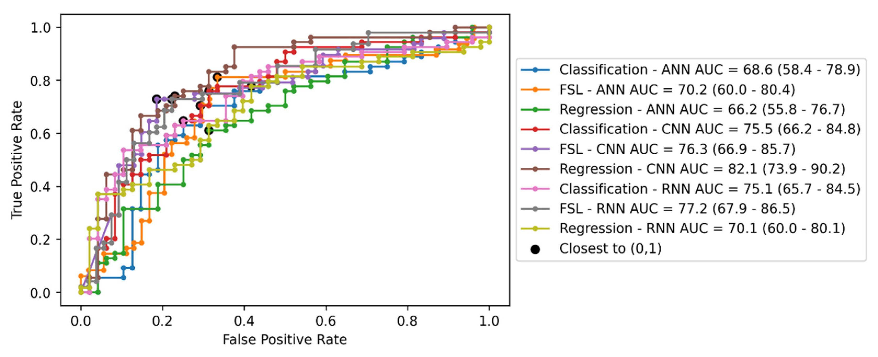
3.2. Invasive FFR Prediction Performance

Figure 2 displays the ROC curve, the AUC scores including their 95% confidence intervals (CI), and the closest point to (0, 1) for all the approaches. The best three approaches based on AUC score are regression CNN, FSL RNN, and FSL CNN. Interestingly, the AUC score is superior for the regression CNN approach, but the FSL CNN approach has the closest point to (0, 1), i.e., the best diagnostic performance statistics, as shown below.
The performance and statistics of the various ensemble DL models and approaches considered herein are displayed in Table 3.
In terms of diagnostic performance, the FSL approach is performing better than classical regression and classification, while in terms of AUC, the CNN regression is superior to other methods. Since the 95% confidence intervals overlap, the differences are statistically not significant. FSL algorithms have been designed for optimal performance on small datasets where they tend to perform better than classic models. The best performing architecture is the one that is based on CNN. Furthermore, the training accuracy suggests that overfitting is not present for eight of the nine approaches. For the classic CNN-based classification, the model seems to overfit, even though different attempts were made to address this: L2 regularization and dropout. The confusion matrix for the best approach is depicted in Table 4.
For comparison, MLD has an accuracy of 67.64%, a sensitivity of 64.81%, and a specificity of 70.83%. The %DS has an accuracy of 63.72%, a sensitivity of 62.96%, and a specificity of 64.58%.
Each ensemble model consists of 20 models that were trained with different seed values. Table 5 displays the mean accuracy, the standard deviation (std) of the accuracy, the minimum accuracy (min), and the maximum accuracy (max) for the validation dataset when employing the default operating points/thresholds of 0.8 for regression and 0.5 for classification. While all variations are quite small, the smallest std is obtained for the models that are based on FSL, which further underlines the robustness of this approach. Additionally, we computed the ensemble model mean uncertainty by averaging the uncertainty of the ensemble model for each examination [66]. The ensemble model uncertainty for regression approaches is the standard deviation of the predictions of all models for one sample. An intuitive approximation for the ensemble model’s uncertainty for classification and FSL approaches was chosen as:
M e a n   e n s a m b l e   u n c e r t a i n t y = i N a b s ( r o u n d ( y ( i ) ) y ( i ) ) N ,  
where y(i) is the ensemble model prediction for each sample and N is the number of samples; this uncertainty measure is the distance between the output probability and the predicted class label (0 or 1), therefore, predictions such as 0.1 or 0.9 are considered “confident” while others such as 0.4 or 0.6 are considered more “uncertain”. This approximation is feasible since ensemble models usually have well-calibrated outputs [66]. The ensemble uncertainty results of the regression approaches are not directly comparable to the ensemble uncertainty results for the classification and FSL approaches, and it has been also shown [66] that regression-based uncertainty that is computed as the ensemble predictions’ standard deviation is not well-calibrated as the MSE training loss “is not a scoring rule that captures predictive uncertainty” [66]. For the regression approaches, RNNs tend to have the smallest uncertainty. For classification and FSL approaches the uncertainty is similar for five of the approaches, while FSL CNN has a much smaller uncertainty.
The reason the default thresholds were employed in Table 5 is that selecting a best-operating-point with respect to some metrics and some held-out test-set is part of a post-processing stage; uncertainty estimates, however, depend solely on two factors: the input samples (i.e., input noise, out-of-distribution, etc.) and the learned model (here, the training procedure, the network architecture, and especially the training set have a large influence); the ground-truth label of a test input sample has no influence on the prediction uncertainty. Therefore, for an unbiased assessment, uncertainty measures of all the approaches were computed from the raw ensemble predictions and compared with the mean accuracy that was obtained from using the default thresholds.
Figure 3 displays four sample cases: one for each of the categories true positive (TP), true negative (TN), false positive (FP), and false negative (FN). A representative angiographic frame is displayed, indicating the invasive FFR value and the coronary vessel and region of interest that is visualized using OCT. Further, the longitudinal OCT view and the radius profile that were used as input to the DNNs are displayed.

3.3. Subgroup Analyses

In the following, we use the best performing model according to the results in Table 3 (FSL-CNN) to perform a series of subgroup analyses.
As detailed in Section 2.1, the dataset contains a large number of samples in the interval 0.75–0.85 (46%). Hence, we have computed the statistics separately for lesions with FFR < 0.75, lesions with FFR > 0.85, and for the lesions with intermediate values. The results are displayed in Table 6. As expected, the accuracy of the model increases in the two bins at the extremes.
In another analysis, we assessed the performance as a function of the vessel on which the measurement was performed. The results are displayed in Table 7 and indicate a higher accuracy on the LCx, compared to the other two main coronary arteries. The literature suggests that the LCx has typically a smaller baseline and hyperemic flow velocity compared to the LAD and RCA, which impacts the FFR measurements [67]. In other words, the same radius profile will lead to different invasive FFR values on different arteries. Since the type of artery is not used as an input to the DNN, a performance difference is expected.
Most of the measurements in the study were performed in the LAD. The clinical literature suggests that proximal LAD lesions are of particular interest for long-term patient outcome [68]. Hence, we have divided LAD lesions into proximal lesions and others (mid or distal lesion). The results are displayed in Table 8 and indicate a similar performance in terms of accuracy, but the sensitivity is slightly lower for proximal lesions. This is an expected outcome since literature indicates that a lesion with a certain severity will lead to smaller FFR values when it is located in the proximal LAD, compared to the mid and distal LAD. Hence, the model slightly underestimates the severity of proximal LAD lesions.
In another analysis, we assessed the prediction performance for male and female patients. The results in Table 9 indicate that the model performs slightly better for male patients. This is an expected outcome since the vast majority of lesions are from male patients (82%).
The age of the patient can be another important factor in the clinical decision-making. We have divided the data at the patient level into three equally large bins. The results in Table 10 indicate a marked difference between the three subgroups. The intermediate bin has a slightly larger number of intermediate lesions (18 vs. 15/14), partially explaining the difference in diagnostic performance.
Finally, in another subgroup analysis we have considered the centerline length of the input data and have divided the samples into three equally sized bins. The results in Table 11 display a balanced performance, i.e., the considered length has no major influence on the model performance.

3.4. Effect of Dataset Size

To assess the impact of the number of samples on the performance, we trained the best performing approach (CNN architecture with FSL) on datasets containing only a part of the original dataset. We started with 30% of the original dataset, and then increased the size in increments of 10%, until reaching 100%, i.e., the original dataset. The smaller datasets were set up by random sampling from the original dataset. To limit the selection bias, for each percentage we ran 20 experiments, where for each experiment a new random sampling was performed, and the CNN was initialized with a new random seed. The accuracy and the standard deviation for all the considered experiments is displayed in Figure 4.
As expected, the dataset size has an important impact on the accuracy. Encouragingly, a relatively linear increase in performance can be observed, indicating that with larger datasets, the performance should further increase. Moreover, the variation, i.e., standard deviation, decreases as the dataset size increases. This is motivated by two aspects. First, the smaller the percentage of data are, the larger is the variability of the actual dataset that is employed for the leave-one-out cross-validation. When 100% of the data are employed, the variability stems only from the random seed that is used for the initialization. Secondly, the larger the dataset, the more robust the prediction will be, i.e., with a smaller variability.

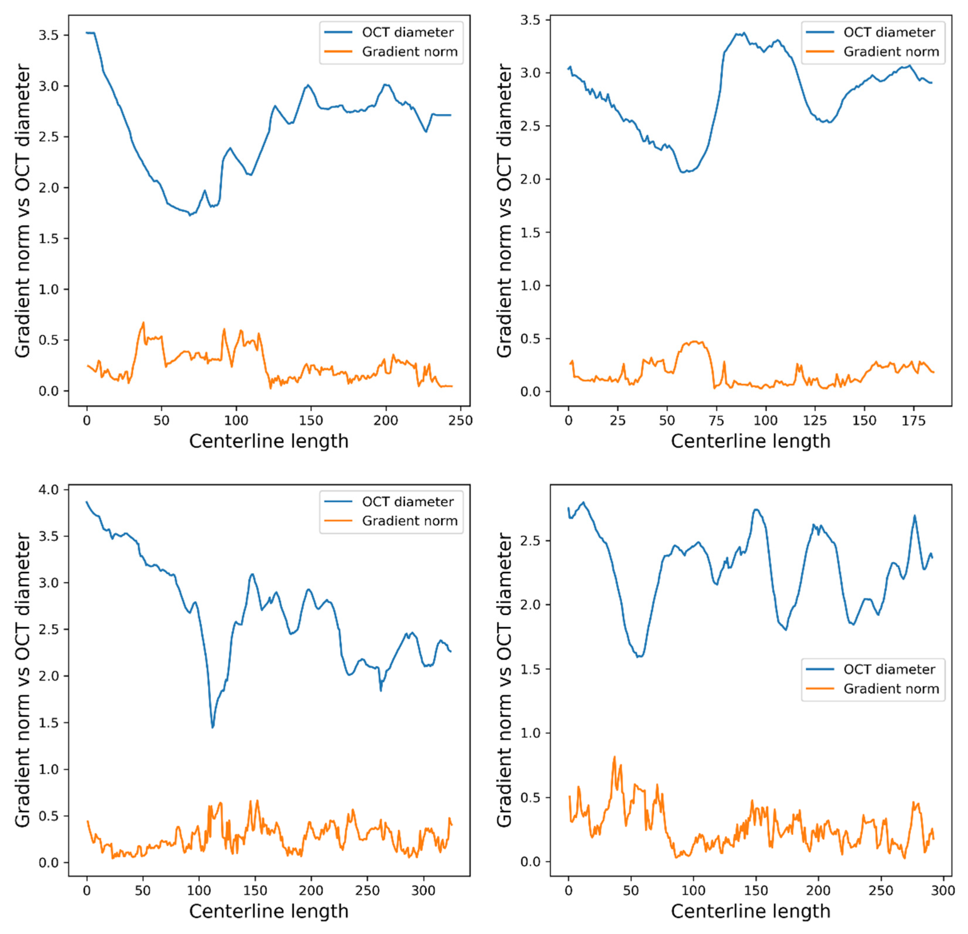
3.5. Saliency Maps and Runtime

To analyze the features that the model is focusing on, we computed the saliency maps [69] for the best ensemble model (CNN-FSL). To obtain the saliency map for the ensemble model, we computed the derivative of the output with respect to the input for each individual model and then we averaged all saliency maps (see Figure 5). As expected, the output of the ensemble CNN-FSL model is influenced by all coronary diameters, but the gradient is larger in the stenosis area, which is known as the main determinant for the measured FFR values.
The training time for one-fold and one epoch is approximately 1050 ms for all the described approaches, the inference time for regression and classification approaches for one sample is approximately 2 ms, and the inference time for FSL approaches for one sample is approximately 25 ms. This difference of one order of magnitude is determined by the necessity of determining the classification clusters. All experiments were run on a desktop computer with AMD Ryzen 9 5900X CPU, 128 GB of RAM, and an NVIDIA RTX 3060 graphics card.

4. Discussion and Conclusions

4.1. Deep Learning-Based Prediction of FFR

As more data are emerging from studies that are based on artificial intelligence and computational modelling, the incremental diagnostic value of predicted coronary functional diagnostic indices over the traditional XA-based visual or quantitative lesion grading is becoming more evident.
We have introduced a method for the deep-learning-based prediction of FFR from routine optical coherence tomography. No specific requirements were formulated for the OCT acquisition. We demonstrated that this approach has a high potential in assessing functionally significant stenoses. Different models and approaches were proposed and evaluated. The experiments indicated the superiority of the FSL-based approach, a type of DL formulation that is specialized for small datasets. However, given the large overlap in the 95% confidence intervals, the differences between the methods are statistically not significant.
Thus, the main findings of this study can be summarized as follows: (1) DL-based FFR prediction from reduced-order raw anatomical data is feasible in a dataset that is focused on intermediate lesions for which the visual anatomical assessment of CAD based on XA does not allow for a clear clinical decision, and with no restriction on the type of lesions that were included in the study, and on the OCT acquisition; (2) DL-based FFR prediction provides superior diagnostic performance compared to baseline approaches based on MLD or %DS; (3) the FFR prediction performance increases quasi-linearly with the dataset size, indicating that a larger training dataset will likely lead to superior diagnostic performance.
The diagnostic accuracy of 77.5% achieved herein is lower compared to that of other studies focusing on FFR prediction from OCT, which reported an accuracy ranging between 88% and 95% [21,22,31,70,71]. There are two main aspects that are responsible for this difference. First, the complexity of the dataset that is processed herein is higher than that of other studies: 46% of the samples have an invasive FFR value ranging between 0.75 and 0.85, while in other studies these grey zone lesions represented between 20% and 44% of the entire dataset [21,22,31,70,71].
Secondly, past studies focusing on FFR prediction from OCT either rely on computational fluid dynamics (CFD) [21,22,70,71], or on ML-based approaches including hand-crafted features [31]. By applying a deep neural network directly on the raw data that are represented by the effective radius along the centerline of the vessel of interest, we allow the model to automatically learn powerful features for FFR prediction. The results that were obtained in other application areas (healthcare or others) demonstrate that classic machine learning (ML) techniques and hand-crafted features typically outperform DL-based approaches when the training set is small, but, conversely, the DL-based approaches outperform classic ML-based approaches when the size of the trainset increases significantly [70]. The results in Figure 4, depicting the accuracy as a function of the dataset size, confirm that a larger dataset will enable a better performance: the performance of the DL model increases quasi-linearly with the dataset size. As shown in Table 3, the diagnostic performance of the proposed model is already considerably higher outside of the 0.75–0.85 FFR value interval.
To increase the prediction performance of DL models, different types of regularization are employed in the literature: mathematical expressions added to the loss function (L1, L2 regularization) [71], dropout (used to randomly drop out neurons during training) [72], and data augmentation [73]. Herein, we have used L2 regularizations and dropout. Data augmentation, i.e., generating new samples by perturbing the input data, is difficult to perform when training against invasively measured FFR, since the approximation of the ground truth values is not straightforward. We have considered data augmentation by adding a small amount of noise to the 1D radius sequence used as input, but the results have not improved.
A DL- or ML-based prediction of FFR was considered also in studies relying on other types of medical images (CCTA, XA). Kumamaru et al. [74] proposed a DL model to estimate invasive FFR from CCTA. They had a dataset containing 207 measurements from 131 patients and have obtained an accuracy of 75.9% in predicting an abnormal invasive FFR (≤0.8). Another interesting approach was proposed by Zreik et al. [75], they used DL in an unsupervised manner and obtained an overall accuracy of 78% on CCTA data. They obtained an accuracy of 66% for FFR < 0.7, 75% for an FFR between 0.7 and 0.8, 79% for an FFR between 0.8 and 0.9, and 73% for an FFR > 0.9. Itu et al. [29] proposed a DL model that was trained on ground truth values computed with a CFD-based approach on a database of synthetically-generated coronary anatomies. They achieved an accuracy of 83.2% on CCTA data.

4.2. Clinical Impact

Despite the overwhelming clinical evidence that an FFR-guided revascularization strategy improves patient outcome, still the number of coronary interventions preceded by FFR measurements is relatively low due to the limitations of invasive pressure measurements [76]. Hence, a virtual functional index would increase the adoption of physiology-guided coronary interventions, while drastically reducing the requirement for invasive pressure measurements.
The proposed method is potentially well suited for a clinical setting, given the real-time prediction performance of the DL model. Certain manual steps are required in the current pipeline, but these can be automated using algorithms for image quality assessment, e.g., to exclude slices with blood artifacts, and more accurate lumen contour detection [77]. The approach only requires knowledge of the coronary luminal geometry, which can be extracted directly from OCT.

4.3. Limitations

The motivation to perform invasive FFR was clinical, which resulted in a large proportion of anatomically borderline lesions in a population with extensive atherosclerotic disease. No cases were excluded, and the results should be interpreted with the consideration that this was a retrospective single-center study.
The anatomical data that was used as input to the DL model may not always accurately reflect the true luminal geometry due to limitations of the OCT acquisition itself (heart motion during automatic pullback, sub-optimal calibration), and small errors that are introduced by the linear interpolation of radius values for the rejected contours. Furthermore, by using the effective radius information as input, we neglect the actual three-dimensional shape of the coronary lumen. The literature suggests that this has a small impact [78], but in certain samples, with non-circular lumen geometry, e.g., concave shape, the impact may not be negligible.
Moreover, the manual editing steps limit the real-time capabilities of the algorithm and introduce intra- and inter-observer variability.
While the subgroup analyses indicate that the length of the considered segment does not influence the results, the maximal length of 7.5 cm may represent a limitation in the case of serial stenoses. For example, if lesions are present in the proximal and distal segment of a vessel, a processed vessel length that is larger than the limit of 7.5 cm would be required to accurately predict FFR.
Finally, to validate our findings and to provide more representative results, the proposed method requires further validation in larger, prospective studies, that are conducted at multiple clinical sites.

4.4. Future Work

Multiple future directions can be defined, given also the current limitations that are listed above. First, the size of the training set should be increased to exploit the capabilities of a deep neural network-based approach. To limit the complexity of the input data, we currently use the effective radius, however, we envision the use of the coronary lumen mask as input, which may then allow the model to consider lumen non-circularities for the prediction. The dimensionality of the input data would increase from 1D to 3D, which would require a larger training set for enabling an accurate prediction. Furthermore, with the increase in the dataset size, other deep-learning approaches (evaluated herein or others) might lead to the best FFR prediction performance.
When employing a classification-based approach, another possible future direction is to increase the number of output classes. For example, a three-class approach would predict lesions as being functionally significant, functionally non-significant, or intermediate/uncertain. This would allow for the definition of hybrid decision-making strategy, where lesions which are not in the intermediate, i.e., uncertain class, can be confidently diagnosed, while for the ones in the intermediate class further aspects may be considered for the final decision, potentially even performing the invasive FFR measurement. The invasive FFR cut-off values for distinguishing the three classes may be chosen based on the performance of the model, e.g., to ensure a sensitivity/specificity of at least 95% for the lesions which are not in the intermediate class. The better the performance of the model, the closer the cut-off values may be to 0.8, i.e., the fewer lesions would be predicted as being uncertain.
Herein, we have considered only the coronary lumen information as input. Previous studies have demonstrated that FFR is influenced also by other patient characteristics (demographics, other pathologies, etc.) [31]. The results of the sub-group analyses have shown the patient sex and age and the vessel of interest may influence the prediction. Additional features may be considered directly as input into the deep neural network, or a cascaded modeling approach may be designed: the first model processes only the coronary lumen information, while the second model, which takes as input the output of the first model, processes all additional features to perform a final and more accurate prediction.
Standard OCT acquisitions have been used for obtaining the input data for the FFR prediction. OCT acquisition guidelines containing specific requirements (e.g., include the entire stenosis in the OCT sequence) may likely improve the prediction accuracy. Such an approach was successfully applied in a previous study [79].
The method that is described herein may be applied similarly on coronary lumen information that is extracted from other imaging modalities (XA, CCTA, IVUS). Since the image resolution, especially on XA and CCTA, is lower than on intra-vascular images, the coronary lumen information may be less accurate. However, XA and CCTA allow for a more complete evaluation of the coronary tree since the vessel of interest can be assessed in all its segments, alongside large side branches. A different methodology might lead to the optimal performance in that case, e.g., based on graph neural networks [80].
Finally, the approach can also be extended to predict other hemodynamic quantities, such as coronary flow reserve (CFR), rest Pd/Pa [81], the instantaneous wave-free ratio (iFR) [82], or hyperemic/basal stenosis resistance (HSR/BSR) [83,84], each of which can be used as a ground-truth during training.

Author Contributions

Conceptualization, C.-A.H., I.-A.T. and L.M.I.; methodology, C.-A.H., C.F.C., I.-A.T. and A.P.; software, C.-A.H., A.P. and D.S.; validation, L.C., N.-M.P.-F., V.B. and A.S.-U.; formal analysis, C.F.C.; investigation, L.C., N.-M.P.-F. and V.B.; resources, I.-A.T. and L.M.I.; data curation, I.-A.T. and L.C.; writing—original draft preparation, C.-A.H., I.-A.T. and L.M.I.; writing—review and editing, C.F.C.; visualization, C.-A.H. and L.M.I.; supervision, L.M.I. and A.S.-U.; project administration, L.M.I. and A.S.-U.; funding acquisition, L.M.I. and A.S.-U. All authors have read and agreed to the published version of the manuscript.

Funding

The research leading to these results has received funding from the EEA Grants 592 2014-2021, under Project contract no. 33/2021. This work was supported by a grant of the Romanian Ministry of Education and Research, CCCDI-UEFISCDI, project number PN-III-P2-2.1-PED-2019-2434, within PNCDI III.

Institutional Review Board Statement

Not applicable.

Informed Consent Statement

Not applicable.

Data Availability Statement

The data has been acquired as part of the projects acknowledged in the manuscript, and cannot be made public, considering GDPR regulations and the content of the informed consent signed by the patients.

Acknowledgments

The concepts and information presented in this paper are based on research results that are not commercially available. Future commercial availability cannot be guaranteed.

Conflicts of Interest

Irina-Andra Tache, Costin Florian Ciusdel, Andrei Puiu, Diana Stoian, and Lucian Mihai Itu are employees of Siemens SRL, Advanta, Brasov, Romania. Cosmin-Andrei Hatfaludi receives a scholarship from Siemens SRL, Advanta, Brasov, Romania. The other authors declare no conflict of interest.

Abbreviations

The following abbreviations are used in the manuscript:
CVD Cardiovascular disease
CADCoronary artery disease
XAX-ray coronary Angiography
OCTOptical coherence tomography
PCI Percutaneous coronary intervention
FFRFractional flow reserve
CABGCoronary artery bypass graft
CFGComputational fluid dynamics
CCTACoronary computed tomography angiography
MLMachine Learning
IVUSIntravascular ultrasound
DNNDeep neural network
DLDeep learning
ANN Artificial neural network
CNNConvolutional neural network
RNNRecurrent neural network
FSLFew-shot learning
ReLURectified linear unit
GRUGated recurrent unit
MLDMinimum lumen diameter
%DSPercentage diameter stenosis
NPVNegative predictive value
PPVPositive predictive value
MAEMean absolute error
MEMean error
MSEMean squared error
LADLeft Anterior Descending artery
LCxLeft Circumflex artery
RCARight Coronary Artery
Arch.Architecture
Corr.Correlation
TPTrue positive
TNTrue negative
FPFalse positive
FNFalse negative
CFRCoronary flow reserve
iFRInstantaneous wave-free ratio
HSRHyperemic stenosis resistance
BSRBasal stenosis resistance
FCFully connected
BCEBinary cross entropy
FoVField of view

Appendix A.

Table A1. ANN architecture. The layer that is highlighted in purple is used only for the regression and the classification approaches (not for the FSL approach). For the regression approach, we used no activation function and the activation function that is highlighted in green is used for the classification approach (not for the FSL approach).
Layer IndexLayerInput FeaturesOutput FeaturesActivation FunctionRegularization
1FC37632ReLU-
2FC3264ReLU-
3FC64128ReLU-
4FC128256ReLUDropout
5FC2561Sigmoid-
Table A2. CNN architecture that is used for the FSL approach.
Layer IndexLayerKernel SizeInput ChannelsOutput ChannelsStrideActivation FunctionRegularizationNormalizationReceptive FoV
1Conv1D31642ReLU-Batch norm3
2Conv1D3641282ReLU-Batch norm7
3Conv1D31282562ReLU-Batch norm15
4Conv1D32565122ReLU-Batch norm31
5Conv1D35125122ReLU-Batch norm63
6Conv1D35125121ReLU-Batch norm127
7Conv1D35125121ReLU-Batch norm191
8Conv1D35125121ReLU-Batch norm255
Table A3. The fully connected layers that were added on top of the architecture that is presented in Table A2, for the CNN-based regression and classification. For the regression approach, we used no activation function and the activation function that is highlighted in green is used for the classification approach (not for the FSL approach).
LayerInput FeaturesOutput FeaturesActivationRegularization
FC20481024ReLUDropout
FC10241Sigmoid-
Table A4. The bidirectional GRU that was added on top of the architecture that is presented in Table A2, used for CNN + RNN approach. The layer that is highlighted in purple is only used for the regression and the classification approach (not for the FSL approach). For the regression approach, we used no activation function and the activation function that is highlighted in green is used for the classification approach (not for the FSL approach).
LayerInput FeaturesHidden SizeOutput FeaturesActivationRegularization
Bidirectional GRU5125121024-Dropout
FC1024-1Sigmoid-

Appendix A.1. Prototypical Networks

Prototypical networks [37] are a subcategory of the embedding learning models. Prototypical networks are used mainly for classification tasks, in both few-shot learning and zero-shot learning scenarios. These neural networks learn a metric space from the data, and then the classification is performed by computing distances to the prototype representations of each class, which are M-dimensional representations of each class cluster, based on an embedding function. They are computed by averaging the embedding vectors of all the training samples of a class (i.e., the neural network features predicted for the input data):
v k = 1 N s i = 1 N s f ϕ ( x i ) ,  
where v k is the prototype of each class, f ϕ is the embedding function, and x i are the support images. The next step consists of classifying the query images. This is performed by computing the distance between each image and the prototypes:
p ϕ ( y = k | x ) = e x p ( d ( f ϕ ( x ) ,   v k ) ) k e x p ( d ( f ϕ ( x ) , v k ) )
During training, the loss is computed using:
J ( ϕ ) = l o g   ( p ϕ ( y = k | x ) )
where k is the true class.

Appendix A.2. Loss Functions

The loss function used for the regression approaches [46] is:
M S E = 1 n i = 1 n ( Y i Y i ) 2 ,  
where Y i is the ground truth value and Y i is the predicted value.
The loss function used for the classification approach [46] (not for FSL the approach):
B C E = 1 n i = 1 n ( Y i · ln   Y i + ( 1 Y i ) · ln ( 1 Y i   ) ) ,  
where Y i is the ground truth value and Y i is the predicted value.
The loss function used for the FSL approaches is described in Equation (A1).

References

  1. Ryan, T.J. The coronary angiogram and its seminal contributions to cardiovascular medicine over five decades. Circulation 2002, 106, 752–756. [Google Scholar] [CrossRef] [PubMed] [Green Version]
  2. Gutierrez-Chico, J.L.; Alegría-Barrero, E.; Teijeiro-Mestre, R.; Chan, P.H.; Tsujioka, H.; de Silva, R.; Viceconte, N.; Lindsay, A.; Patterson, T.; Foin, N. Optical coherence tomography: From research to practice. Eur. Heart J.-Cardiovasc. Imaging 2012, 13, 370–384. [Google Scholar] [CrossRef]
  3. Gutiérrez-Chico, J.L.; Regar, E.; Nüesch, E.; Okamura, T.; Wykrzykowska, J.; di Mario, C.; Windecker, S.; van Es, G.-A.; Gobbens, P.; Jüni, P. Delayed coverage in malapposed and side-branch struts with respect to well-apposed struts in drug-eluting stents: In vivo assessment with optical coherence tomography. Circulation 2011, 124, 612–623. [Google Scholar] [CrossRef] [PubMed] [Green Version]
  4. Gutiérrez-Chico, J.L.; Wykrzykowska, J.; Nüesch, E.; van Geuns, R.J.; Koch, K.T.; Koolen, J.J.; di Mario, C.; Windecker, S.; van Es, G.-A.; Gobbens, P. Vascular tissue reaction to acute malapposition in human coronary arteries: Sequential assessment with optical coherence tomography. Circ. Cardiovasc. Interv. 2012, 5, 20–29. [Google Scholar] [CrossRef] [PubMed] [Green Version]
  5. Ali, Z.A.; Maehara, A.; Généreux, P.; Shlofmitz, R.A.; Fabbiocchi, F.; Nazif, T.M.; Guagliumi, G.; Meraj, P.M.; Alfonso, F.; Samady, H. Optical coherence tomography compared with intravascular ultrasound and with angiography to guide coronary stent implantation (ILUMIEN III: OPTIMIZE PCI): A randomised controlled trial. Lancet 2016, 388, 2618–2628. [Google Scholar] [CrossRef]
  6. Gonzalo, N.; Escaned, J.; Alfonso, F.; Nolte, C.; Rodriguez, V.; Jimenez-Quevedo, P.; Bañuelos, C.; Fernández-Ortiz, A.; Garcia, E.; Hernandez-Antolin, R. Morphometric assessment of coronary stenosis relevance with optical coherence tomography: A comparison with fractional flow reserve and intravascular ultrasound. J. Am. Coll. Cardiol. 2012, 59, 1080–1089. [Google Scholar] [CrossRef] [PubMed] [Green Version]
  7. Pijls, N.H.; de Bruyne, B.; Peels, K.; van der Voort, P.H.; Bonnier, H.J.; Bartunek, J.; Koolen, J.J. Measurement of fractional flow reserve to assess the functional severity of coronary-artery stenoses. N. Engl. J. Med. 1996, 334, 1703–1708. [Google Scholar] [CrossRef] [PubMed]
  8. Tonino, P.A.; De Bruyne, B.; Pijls, N.H.; Siebert, U.; Ikeno, F.; vant Veer, M.; Klauss, V.; Manoharan, G.; Engstrøm, T.; Oldroyd, K.G. Fractional flow reserve versus angiography for guiding percutaneous coronary intervention. N. Engl. J. Med. 2009, 360, 213–224. [Google Scholar] [CrossRef] [Green Version]
  9. Tu, S.; Bourantas, C.V.; Nørgaard, B.L.; Kassab, G.S.; Koo, B.K.; Reiber, J. Image-based assessment of fractional flow reserve. EuroIntervention J. EuroPCR Collab. Work. Group Interv. Cardiol. Eur. Soc. Cardiol. 2015, 11, V50–V54. [Google Scholar] [CrossRef]
  10. Yang, D.H.; Kim, Y.-H.; Roh, J.H.; Kang, J.-W.; Ahn, J.-M.; Kweon, J.; Lee, J.B.; Choi, S.H.; Shin, E.-S.; Park, D.-W. Diagnostic performance of on-site CT-derived fractional flow reserve versus CT perfusion. Eur. Heart J.-Cardiovasc. Imaging 2017, 18, 432–440. [Google Scholar] [CrossRef] [Green Version]
  11. Coenen, A.; Lubbers, M.M.; Kurata, A.; Kono, A.; Dedic, A.; Chelu, R.G.; Dijkshoorn, M.L.; Gijsen, F.J.; Ouhlous, M.; van Geuns, R.-J.M. Fractional flow reserve computed from noninvasive CT angiography data: Diagnostic performance of an on-site clinician-operated computational fluid dynamics algorithm. Radiology 2015, 274, 674–683. [Google Scholar] [CrossRef] [PubMed]
  12. Renker, M.; Schoepf, U.J.; Wang, R.; Meinel, F.G.; Rier, J.D.; Bayer II, R.R.; Möllmann, H.; Hamm, C.W.; Steinberg, D.H.; Baumann, S. Comparison of diagnostic value of a novel noninvasive coronary computed tomography angiography method versus standard coronary angiography for assessing fractional flow reserve. Am. J. Cardiol. 2014, 114, 1303–1308. [Google Scholar] [CrossRef] [PubMed]
  13. Koo, B.-K.; Erglis, A.; Doh, J.-H.; Daniels, D.V.; Jegere, S.; Kim, H.-S.; Dunning, A.; DeFrance, T.; Lansky, A.; Leipsic, J. Diagnosis of ischemia-causing coronary stenoses by noninvasive fractional flow reserve computed from coronary computed tomographic angiograms: Results from the prospective multicenter DISCOVER-FLOW (Diagnosis of Ischemia-Causing Stenoses Obtained Via Noninvasive Fractional Flow Reserve) study. J. Am. Coll. Cardiol. 2011, 58, 1989–1997. [Google Scholar]
  14. Tu, S.; Westra, J.; Yang, J.; von Birgelen, C.; Ferrara, A.; Pellicano, M.; Nef, H.; Tebaldi, M.; Murasato, Y.; Lansky, A. Diagnostic accuracy of fast computational approaches to derive fractional flow reserve from diagnostic coronary angiography: The international multicenter FAVOR pilot study. Cardiovasc. Interv. 2016, 9, 2024–2035. [Google Scholar]
  15. Tröbs, M.; Achenbach, S.; Röther, J.; Redel, T.; Scheuering, M.; Winneberger, D.; Klingenbeck, K.; Itu, L.; Passerini, T.; Kamen, A. Comparison of fractional flow reserve based on computational fluid dynamics modeling using coronary angiographic vessel morphology versus invasively measured fractional flow reserve. Am. J. Cardiol. 2016, 117, 29–35. [Google Scholar] [CrossRef]
  16. Papafaklis, M.I.; Muramatsu, T.; Ishibashi, Y.; Lakkas, L.S.; Nakatani, S.; Bourantas, C.V.; Ligthart, J.; Onuma, Y.; Echavarria-Pinto, M.; Tsirka, G. Fast virtual functional assessment of intermediate coronary lesions using routine angiographic data and blood flow simulation in humans: Comparison with pressure wire-fractional flow reserve. EuroIntervention 2014, 10, 574–583. [Google Scholar] [CrossRef]
  17. Tu, S.; Barbato, E.; Köszegi, Z.; Yang, J.; Sun, Z.; Holm, N.R.; Tar, B.; Li, Y.; Rusinaru, D.; Wijns, W. Fractional flow reserve calculation from 3-dimensional quantitative coronary angiography and TIMI frame count: A fast computer model to quantify the functional significance of moderately obstructed coronary arteries. JACC Cardiovasc. Interv. 2014, 7, 768–777. [Google Scholar] [CrossRef] [Green Version]
  18. Morris, P.D.; Ryan, D.; Morton, A.C.; Lycett, R.; Lawford, P.V.; Hose, D.R.; Gunn, J.P. Virtual fractional flow reserve from coronary angiography: Modeling the significance of coronary lesions: Results from the VIRTU-1 (VIRTUal Fractional Flow Reserve From Coronary Angiography) study. JACC Cardiovasc. Interv. 2013, 6, 149–157. [Google Scholar] [CrossRef] [PubMed] [Green Version]
  19. Seike, F.; Uetani, T.; Nishimura, K.; Kawakami, H.; Higashi, H.; Aono, J.; Nagai, T.; Inoue, K.; Suzuki, J.; Kawakami, H. Intracoronary optical coherence tomography-derived virtual fractional flow reserve for the assessment of coronary artery disease. Am. J. Cardiol. 2017, 120, 1772–1779. [Google Scholar] [CrossRef]
  20. Jang, S.-J.; Ahn, J.-M.; Kim, B.; Gu, J.-M.; Sung, H.J.; Park, S.-J.; Oh, W.-Y. Comparison of accuracy of one-use methods for calculating fractional flow reserve by intravascular optical coherence tomography to that determined by the pressure-wire method. Am. J. Cardiol. 2017, 120, 1920–1925. [Google Scholar] [CrossRef]
  21. Yu, W.; Huang, J.; Jia, D.; Chen, S.; Raffel, O.C.; Ding, D.; Tian, F.; Kan, J.; Zhang, S.; Yan, F. Diagnostic accuracy of intracoronary optical coherence tomography-derived fractional flow reserve for assessment of coronary stenosis severity. EuroIntervention J. EuroPCR Collab. Work. Group Interv. Cardiol. Eur. Soc. Cardiol. 2019, 15, 189. [Google Scholar] [CrossRef] [PubMed] [Green Version]
  22. Ha, J.; Kim, J.-S.; Lim, J.; Kim, G.; Lee, S.; Lee, J.S.; Shin, D.-H.; Kim, B.-K.; Ko, Y.-G.; Choi, D. Assessing computational fractional flow reserve from optical coherence tomography in patients with intermediate coronary stenosis in the left anterior descending artery. Circ. Cardiovasc. Interv. 2016, 9, e003613. [Google Scholar] [CrossRef] [PubMed]
  23. Itu, L.; Sharma, P.; Mihalef, V.; Kamen, A.; Suciu, C.; Lomaniciu, D. A patient-specific reduced-order model for coronary circulation. In Proceedings of the 2012 9th IEEE International Symposium on Biomedical Imaging (ISBI), Barcelona, Spain, 2–5 May 2012; pp. 832–835. [Google Scholar]
  24. Deng, S.-B.; Jing, X.-D.; Wang, J.; Huang, C.; Xia, S.; Du, J.-L.; Liu, Y.-J.; She, Q. Diagnostic performance of noninvasive fractional flow reserve derived from coronary computed tomography angiography in coronary artery disease: A systematic review and meta-analysis. Int. J. Cardiol. 2015, 184, 703–709. [Google Scholar] [CrossRef]
  25. Bishop, C.M.; Nasrabadi, N.M. Pattern Recognition and Machine Learning; Springer: Berlin/Heidelberg, Germany, 2006; Volume 4. [Google Scholar]
  26. Zheng, Y.; Comaniciu, D. Marginal Space Learning for Medical Image Analysis; Springer: Berlin/Heidelberg, Germany, 2014; Volume 2, p. 6. [Google Scholar]
  27. Mansi, T.; Georgescu, B.; Hussan, J.; Hunter, P.J.; Kamen, A.; Comaniciu, D. Data-driven reduction of a cardiac myofilament model. In Proceedings of the International Conference on Functional Imaging and Modeling of the Heart, London, UK, 20–22 June 2013; pp. 232–240. [Google Scholar]
  28. Tøndel, K.; Indahl, U.G.; Gjuvsland, A.B.; Vik, J.O.; Hunter, P.; Omholt, S.W.; Martens, H. Hierarchical Cluster-based Partial Least Squares Regression (HC-PLSR) is an efficient tool for metamodelling of nonlinear dynamic models. BMC Syst. Biol. 2011, 5, 90. [Google Scholar] [CrossRef] [PubMed] [Green Version]
  29. Itu, L.; Rapaka, S.; Passerini, T.; Georgescu, B.; Schwemmer, C.; Schoebinger, M.; Flohr, T.; Sharma, P.; Comaniciu, D. A machine-learning approach for computation of fractional flow reserve from coronary computed tomography. J. Appl. Physiol. 2016, 121, 42–52. [Google Scholar] [CrossRef] [PubMed] [Green Version]
  30. Cho, H.; Lee, J.G.; Kang, S.J.; Kim, W.J.; Choi, S.Y.; Ko, J.; Min, H.S.; Choi, G.H.; Kang, D.Y.; Lee, P.H. Angiography-based machine learning for predicting fractional flow reserve in intermediate coronary artery lesions. J. Am. Heart Assoc. 2019, 8, e011685. [Google Scholar] [CrossRef] [PubMed] [Green Version]
  31. Cha, J.-J.; Son, T.D.; Ha, J.; Kim, J.-S.; Hong, S.-J.; Ahn, C.-M.; Kim, B.-K.; Ko, Y.-G.; Choi, D.; Hong, M.-K. Optical coherence tomography-based machine learning for predicting fractional flow reserve in intermediate coronary stenosis: A feasibility study. Sci. Rep. 2020, 10, 20421. [Google Scholar] [CrossRef] [PubMed]
  32. Lee, J.-G.; Ko, J.; Hae, H.; Kang, S.-J.; Kang, D.-Y.; Lee, P.H.; Ahn, J.-M.; Park, D.-W.; Lee, S.-W.; Kim, Y.-H. Intravascular ultrasound-based machine learning for predicting fractional flow reserve in intermediate coronary artery lesions. Atherosclerosis 2020, 292, 171–177. [Google Scholar] [CrossRef]
  33. Deng, L.; Yu, D. Deep learning: Methods and applications. Found. Trends Signal Processing 2014, 7, 197–387. [Google Scholar] [CrossRef] [Green Version]
  34. LeCun, Y.; Bengio, Y.; Hinton, G. Deep learning. Nature 2015, 521, 436–444. [Google Scholar] [CrossRef]
  35. Wang, Y.; Yao, Q.; Kwok, J.T.; Ni, L.M. Generalizing from a few examples: A survey on few-shot learning. ACM Comput. Surv. 2020, 53, 1–34. [Google Scholar] [CrossRef]
  36. Jiang, X.; Zeng, Y.; Xiao, S.; He, S.; Ye, C.; Qi, Y.; Zhao, J.; Wei, D.; Hu, M.; Chen, F. Automatic detection of coronary metallic stent struts based on YOLOv3 and R-FCN. Comput. Math. Methods Med. 2020, 2020, 1793517. [Google Scholar] [CrossRef]
  37. Wang, Z.; Jenkins, M.W.; Linderman, G.C.; Bezerra, H.G.; Fujino, Y.; Costa, M.A.; Wilson, D.L.; Rollins, A.M. 3-D stent detection in intravascular OCT using a Bayesian network and graph search. IEEE Trans. Med. Imaging 2015, 34, 1549–1561. [Google Scholar] [CrossRef] [PubMed]
  38. Wu, P.; Gutiérrez-Chico, J.L.; Tauzin, H.; Yang, W.; Li, Y.; Yu, W.; Chu, M.; Guillon, B.; Bai, J.; Meneveau, N. Automatic stent reconstruction in optical coherence tomography based on a deep convolutional model. Biomed. Opt. Express 2020, 11, 3374–3394. [Google Scholar] [CrossRef] [PubMed]
  39. Yang, G.; Mehanna, E.; Li, C.; Zhu, H.; He, C.; Lu, F.; Zhao, K.; Gong, Y.; Wang, Z. Stent detection with very thick tissue coverage in intravascular OCT. Biomed. Opt. Express 2021, 12, 7500–7516. [Google Scholar] [CrossRef] [PubMed]
  40. Lau, Y.S.; Tan, L.K.; Chan, C.K.; Chee, K.H.; Liew, Y.M. Automated segmentation of metal stent and bioresorbable vascular scaffold in intravascular optical coherence tomography images using deep learning architectures. Phys. Med. Biol. 2021, 66, 245026. [Google Scholar] [CrossRef]
  41. Lee, J.; Gharaibeh, Y.; Kolluru, C.; Zimin, V.N.; Dallan, L.A.P.; Kim, J.N.; Bezerra, H.G.; Wilson, D.L. Segmentation of Coronary Calcified Plaque in Intravascular OCT Images Using a Two-Step Deep Learning Approach. IEEE Access 2020, 8, 225581–225593. [Google Scholar] [CrossRef]
  42. Gharaibeh, Y.; Prabhu, D.S.; Kolluru, C.; Lee, J.; Zimin, V.; Bezerra, H.G.; Wilson, D.L. Coronary calcification segmentation in intravascular OCT images using deep learning: Application to calcification scoring. J. Med. Imaging 2019, 6, 045002. [Google Scholar] [CrossRef] [Green Version]
  43. Abdolmanafi, A.; Duong, L.; Ibrahim, R.; Dahdah, N. A deep learning-based model for characterization of atherosclerotic plaque in coronary arteries using optical coherence tomography images. Med. Phys. 2021, 48, 3511–3524. [Google Scholar] [CrossRef]
  44. Pociask, E.; Malinowski, K.P.; Ślęzak, M.; Jaworek-Korjakowska, J.; Wojakowski, W.; Roleder, T. Fully automated lumen segmentation method for intracoronary optical coherence tomography. J. Healthc. Eng. 2018, 2018, 1414076. [Google Scholar] [CrossRef] [Green Version]
  45. Jiao, C.; Xu, Z.; Bian, Q.; Forsberg, E.; Tan, Q.; Peng, X.; He, S. Machine learning classification of origins and varieties of Tetrastigma hemsleyanum using a dual-mode microscopic hyperspectral imager. Spectrochim. Acta Part A Mol. Biomol. Spectrosc. 2021, 261, 120054. [Google Scholar] [CrossRef] [PubMed]
  46. Wang, T.; Shen, F.; Deng, H.; Cai, F.; Chen, S. Smartphone imaging spectrometer for egg/meat freshness monitoring. Anal. Methods 2022, 14, 508–517. [Google Scholar] [CrossRef] [PubMed]
  47. Snell, J.; Swersky, K.; Zemel, R. Prototypical networks for few-shot learning. Adv. Neural Inf. Processing Syst. 2017, 30. [Google Scholar]
  48. Kern, M.J.; Lerman, A.; Bech, J.-W.; De Bruyne, B.; Eeckhout, E.; Fearon, W.F.; Higano, S.T.; Lim, M.J.; Meuwissen, M.; Piek, J.J. Physiological assessment of coronary artery disease in the cardiac catheterization laboratory: A scientific statement from the American Heart Association Committee on Diagnostic and Interventional Cardiac Catheterization, Council on Clinical Cardiology. Circulation 2006, 114, 1321–1341. [Google Scholar] [CrossRef] [PubMed] [Green Version]
  49. Bradski, G. The openCV library. Dr. Dobb’s J. Softw. Tools Prof. Program. 2000, 25, 120–123. [Google Scholar]
  50. Patro, S.; Sahu, K.K. Normalization: A preprocessing stage. arXiv 2015, arXiv:1503.06462. [Google Scholar] [CrossRef]
  51. Agarap, A.F. Deep learning using rectified linear units (relu). arXiv 2018, arXiv:1803.08375. [Google Scholar]
  52. Santurkar, S.; Tsipras, D.; Ilyas, A.; Madry, A. How does batch normalization help optimization? Adv. Neural Inf. Processing Syst. 2018, 31. [Google Scholar]
  53. Dey, R.; Salem, F.M. Gate-variants of gated recurrent unit (GRU) neural networks. In Proceedings of the 2017 IEEE 60th International Midwest Symposium on Circuits and Systems (MWSCAS), Boston, MA, USA, 6–9 August 2017; pp. 1597–1600. [Google Scholar]
  54. Han, J.; Moraga, C. The influence of the sigmoid function parameters on the speed of backpropagation learning. In Proceedings of the International Workshop on Artificial Neural Networks, Malaga-Torremolinos, Spain, 7–9 June 1995; pp. 195–201. [Google Scholar]
  55. Wong, T.-T. Performance evaluation of classification algorithms by k-fold and leave-one-out cross validation. Pattern Recognit. 2015, 48, 2839–2846. [Google Scholar] [CrossRef]
  56. Zhang, Z. Improved adam optimizer for deep neural networks. In Proceedings of the 2018 IEEE/ACM 26th International Symposium on Quality of Service (IWQoS), Banff, AB, Canada, 4–6 June 2018; pp. 1–2. [Google Scholar]
  57. Kline, D.M.; Berardi, V.L. Revisiting squared-error and cross-entropy functions for training neural network classifiers. Neural Comput. Appl. 2005, 14, 310–318. [Google Scholar] [CrossRef]
  58. Liashchynskyi, P.; Liashchynskyi, P. Grid search, random search, genetic algorithm: A big comparison for NAS. arXiv 2019, arXiv:1912.06059. [Google Scholar]
  59. Paszke, A.; Gross, S.; Massa, F.; Lerer, A.; Bradbury, J.; Chanan, G.; Killeen, T.; Lin, Z.; Gimelshein, N.; Antiga, L. Pytorch: An imperative style, high-performance deep learning library. Adv. Neural Inf. Processing Syst. 2019, 32. [Google Scholar]
  60. Hoo, Z.H.; Candlish, J.; Teare, D. What is an ROC curve? Emerg. Med. J. 2017, 34, 357–359. [Google Scholar] [CrossRef] [PubMed]
  61. Lobo, J.M.; Jiménez-Valverde, A.; Real, R. AUC: A misleading measure of the performance of predictive distribution models. Glob. Ecol. Biogeogr. 2008, 17, 145–151. [Google Scholar] [CrossRef]
  62. Unal, I. Defining an optimal cut-point value in ROC analysis: An alternative approach. Comput. Math. Methods Med. 2017, 2017, 3762651. [Google Scholar] [CrossRef] [PubMed]
  63. Youden, W.J. Index for rating diagnostic tests. Cancer 1950, 3, 32–35. [Google Scholar] [CrossRef]
  64. Wong, H.B.; Lim, G.H. Measures of diagnostic accuracy: Sensitivity, specificity, PPV and NPV. Proc. Singap. Healthc. 2011, 20, 316–318. [Google Scholar] [CrossRef]
  65. Genders, T.S.; Spronk, S.; Stijnen, T.; Steyerberg, E.W.; Lesaffre, E.; Hunink, M.M. Methods for calculating sensitivity and specificity of clustered data: A tutorial. Radiology 2012, 265, 910–916. [Google Scholar] [CrossRef]
  66. Lakshminarayanan, B.; Pritzel, A.; Blundell, C. Simple and scalable predictive uncertainty estimation using deep ensembles. Adv. Neural Inf. Processing Syst. 2017, 30. [Google Scholar]
  67. Wieneke, H.; Von Birgelen, C.; Haude, M.; Eggebrecht, H.; Mohlenkamp, S.; Schmermund, A.; Bose, D.; Altmann, C.; Bartel, T.; Erbel, R. Determinants of coronary blood flow in humans: Quantification by intracoronary Doppler and ultrasound. J. Appl. Physiol. 2005, 98, 1076–1082. [Google Scholar] [CrossRef] [Green Version]
  68. Kobayashi, Y.; Johnson, N.P.; Berry, C.; De Bruyne, B.; Gould, K.L.; Jeremias, A.; Oldroyd, K.G.; Pijls, N.H.; Fearon, W.F.; Investigators, C.S. The influence of lesion location on the diagnostic accuracy of adenosine-free coronary pressure wire measurements. JACC Cardiovasc. Interv. 2016, 9, 2390–2399. [Google Scholar] [CrossRef] [PubMed]
  69. Simonyan, K.; Vedaldi, A.; Zisserman, A. Deep inside convolutional networks: Visualising image classification models and saliency maps. arXiv 2013, arXiv:1312.6034. [Google Scholar]
  70. Bote-Curiel, L.; Munoz-Romero, S.; Gerrero-Curieses, A.; Rojo-Álvarez, J.L. Deep learning and big data in healthcare: A double review for critical beginners. Appl. Sci. 2019, 9, 2331. [Google Scholar] [CrossRef] [Green Version]
  71. Demir-Kavuk, O.; Kamada, M.; Akutsu, T.; Knapp, E.-W. Prediction using step-wise L1, L2 regularization and feature selection for small data sets with large number of features. BMC Bioinform. 2011, 12, 412. [Google Scholar] [CrossRef] [PubMed] [Green Version]
  72. Srivastava, N.; Hinton, G.; Krizhevsky, A.; Sutskever, I.; Salakhutdinov, R. Dropout: A simple way to prevent neural networks from overfitting. J. Mach. Learn. Res. 2014, 15, 1929–1958. [Google Scholar]
  73. Wong, S.C.; Gatt, A.; Stamatescu, V.; McDonnell, M.D. Understanding data augmentation for classification: When to warp? In Proceedings of the 2016 International Conference on Digital Image Computing: Techniques and Applications (DICTA), Gold Coast, Australia, 30 November–2 December 2016; pp. 1–6. [Google Scholar]
  74. Kumamaru, K.K.; Fujimoto, S.; Otsuka, Y.; Kawasaki, T.; Kawaguchi, Y.; Kato, E.; Takamura, K.; Aoshima, C.; Kamo, Y.; Kogure, Y. Diagnostic accuracy of 3D deep-learning-based fully automated estimation of patient-level minimum fractional flow reserve from coronary computed tomography angiography. Eur. Heart J.-Cardiovasc. Imaging 2020, 21, 437–445. [Google Scholar] [CrossRef] [PubMed] [Green Version]
  75. Zreik, M.; van Hamersvelt, R.W.; Khalili, N.; Wolterink, J.M.; Voskuil, M.; Viergever, M.A.; Leiner, T.; Išgum, I. Deep learning analysis of coronary arteries in cardiac CT angiography for detection of patients requiring invasive coronary angiography. IEEE Trans. Med. Imaging 2019, 39, 1545–1557. [Google Scholar] [CrossRef] [Green Version]
  76. Petraco, R.; Park, J.J.; Sen, S.; Nijjer, S.; Malik, I.; Pinto, M.E.; Asrress, K.; Nam, C.W.; Foale, R.; Sethi, A. Hybrid iFR-FFR decision-making strategy: Implications for enhancing universal adoption of physiology-guided coronary revascularization. Am. J. Cardiol. 2013, 111, 54B. [Google Scholar] [CrossRef]
  77. Guo, X.; Tang, D.; Molony, D.; Yang, C.; Samady, H.; Zheng, J.; Mintz, G.S.; Maehara, A.; Wang, L.; Pei, X. A machine learning-based method for intracoronary oct segmentation and vulnerable coronary plaque cap thickness quantification. Int. J. Comput. Methods 2019, 16, 1842008. [Google Scholar] [CrossRef]
  78. Lyras, K.G.; Lee, J. An improved reduced-order model for pressure drop across arterial stenoses. PLoS ONE 2021, 16, e0258047. [Google Scholar] [CrossRef]
  79. Gutiérrez-Chico, J.L.; Chen, Y.; Yu, W.; Ding, D.; Huang, J.; Huang, P.; Jing, J.; Chu, M.; Wu, P.; Tian, F. Diagnostic accuracy and reproducibility of optical flow ratio for functional evaluation of coronary stenosis in a prospective series. Cardiol. J. 2020, 27, 350–361. [Google Scholar] [CrossRef] [PubMed]
  80. Georgousis, S.; Kenning, M.P.; Xie, X. Graph deep learning: State of the art and challenges. IEEE Access 2021, 9, 22106–22140. [Google Scholar] [CrossRef]
  81. Kern, M.J. Coronary physiology revisited: Practical insights from the cardiac catheterization laboratory. Circulation 2000, 101, 1344–1351. [Google Scholar] [CrossRef] [PubMed] [Green Version]
  82. Sen, S.; Escaned, J.; Malik, I.S.; Mikhail, G.W.; Foale, R.A.; Mila, R.; Tarkin, J.; Petraco, R.; Broyd, C.; Jabbour, R. Development and validation of a new adenosine-independent index of stenosis severity from coronary wave–intensity analysis: Results of the ADVISE (ADenosine Vasodilator Independent Stenosis Evaluation) study. J. Am. Coll. Cardiol. 2012, 59, 1392–1402. [Google Scholar] [CrossRef] [Green Version]
  83. Meuwissen, M.; Siebes, M.; Chamuleau, S.A.; van Eck-Smit, B.L.; Koch, K.T.; de Winter, R.J.; Tijssen, J.G.; Spaan, J.A.; Piek, J.J. Hyperemic stenosis resistance index for evaluation of functional coronary lesion severity. Circulation 2002, 106, 441–446. [Google Scholar] [CrossRef] [Green Version]
  84. van de Hoef, T.P.; Nolte, F.; Damman, P.; Delewi, R.; Bax, M.; Chamuleau, S.A.; Voskuil, M.; Siebes, M.; Tijssen, J.G.; Spaan, J.A. Diagnostic accuracy of combined intracoronary pressure and flow velocity information during baseline conditions: Adenosine-free assessment of functional coronary lesion severity. Circ. Cardiovasc. Interv. 2012, 5, 508–514. [Google Scholar] [CrossRef] [Green Version]
Figure 1. OCT data processing workflow, including FFR prediction using a deep neural network.
Applsci 12 06964 g001
Figure 2. The ROC curve, AUC score, and the closest point to (0, 1) for all approaches. Values in the parentheses represent the 95% confidence intervals computed as in [65].
Applsci 12 06964 g002
Figure 3. Four sample cases: one for each of the categories: (a) TP, (b) TN, (c) FP, and (d) FN. A representative angiographic frame is displayed indicating the invasive FFR value and the coronary vessel and region of interest visualized using OCT. The longitudinal OCT view and the radius profile used as input to the DNNs are also displayed.
Applsci 12 06964 g003
Figure 4. Model accuracy as a function of the dataset size.
Applsci 12 06964 g004
Figure 5. The saliency map that was computed for the ensemble CNN-FSL model. The saliency maps on the top correspond to samples with an invasive FFR > 0.8, and the saliency maps on the bottom correspond to samples with an invasive FFR < 0.8.
Applsci 12 06964 g005
Table 1. Baseline patient characteristics and risk factors (n = 80).
Male66 (82%)
Female14 (18%)
Age (years)60.5 ± 11.2 years
RaceAll Caucasian
Weight81.93 ± 16.15 kg
Height172.13 ± 8.05 cm
Diabetes27 (33.75%)
Hypertension60 (75%)
Hypercholesterolemia62 (77.5%)
Smoking history42 (52.5%)
Family history of CAD3 (2.9%)
Previous myocardial infarction46 (45%)
Previous Angina64 (80%)
Ejection fraction48.28 ± 6.31%
Table 2. Baseline lesion characteristics (n = 102).
Index Artery
Left Anterior Descending artery (LAD)57
Left Circumflex artery (LCx)20
Right Coronary Artery (RCA)25
Fractional Flow Reserve
Mean ± SD0.80 ± 0.08
Median (IQR)0.83 (0.75−0.86)
FFR ≤ 0.8048
FFR < 0.7525
0.75 ≤ FFR ≤ 0.8547
FFR > 0.8530
Table 3. Diagnostics and performance statistics of the considered ensemble DL models and approaches. Values in the parentheses represent the 95% confidence intervals.
Validation
ApproachEnsemble Arch.Train_Accuracy
[%]
Accuracy
[%]
Sensitivity
[%]
Specificity
[%]
NPV
[%]
PPV
[%]
AUC
[%]
MAEMEMSECorr.
RegressionANN73.764.7 (55.1–73.3)61.1 (47.8–80.1)68.8 (54.7–80.1)61.1 (47.8–73.0)68.8 (54.7–80.1)66.2 (55.8–76.7)0.0620.0070.1050.273
CNN85.975.5 (66.3–82.8)74.1 (61.1–86.7)77.1 (63.5–86.7)72.5 (59.1–82.9)78.4 (65.4–87.5)82.1 (73.9–90.2)0.082−0.0080.0150.342
RNN69.768.6 (59.1–76.8)77.8 (65.1–71.2)58.3 (44.3–71.2)70.0 (54.6–81.9)67.7 (55.4–78.0)70.1 (60–80.1)0.0720.0220.0110.261
ClassificationANN78.470.6 (61.1–78.6)70.4 (57.2–81.8)70.8 (56.8–81.8)68.0 (54.2–79.2)73.1 (59.7–83.2)68.6 (58.4–78.9)----
CNN98.772.5 (63.2–80.3)75.9 (63.1–80.1)68.8 (54.7–80.1)71.7 (57.5–82.7)73.2 (60.4–83.0)75.5 (66.2–84.8)----
RNN73.869.6 (60.1–77.7)64.8 (51.5–85.1)75.0 (61.2–85.1)65.5 (52.3–76.6)74.5 (60.5–84.7)75.1 (65.7–74.5)----
FSLANN78.972.5 (63.2–80.3)79.2 (65.7–77.8)66.7 (53.4–77.8)78.3 (64.4–87.7)67.9 (54.8–78.6)70.2 (60–80.4)----
CNN78.677.5 (68.4–84.5)72.9 (59.0–89.6)81.5 (69.2–89.6)77.2 (64.8–86.2)77.8 (63.7–87.5)76.3 (66.9–85.7)----
RNN75.675.5 (66.3–82.8)72.9 (59.0–86.8)77.8 (65.1–86.8)76.4 (63.7–85.6)74.5 (60.5–84.7)77.2 (60–80.1)----
Table 4. The confusion matrix for the FSL-CNN approach.
Predicted Values Actual Values
Positive (1)Negative (0)
Positive (1)3513
Negative (0)1144
Table 5. Diagnostic performance statistics of the considered ensemble DL models and approaches.
Accuracy
ApproachEnsemble Arch.Mean
[%]
Std
[%]
Min
[%]
Max
[%]
Uncertainty
[%]
RegressionANN61.574.5553.9270.594.48
CNN61.762.6555.8865.6912.91
RNN63.193.8254.971.572.25
ClassificationANN68.431.6965.6972.5532.55
CNN67.753.163.7373.5332.9
RNN68.041.7164.7171.5731.69
FSLANN66.673.3459.872.5530.9
CNN75.591.272.5576.472.77
RNN74.461.3771.5776.4734.71
Table 6. Diagnostic performance and 95% CI of the model for lesions with FFR < 0.75, lesions with FFR > 0.85, and for the lesions with intermediate values.
FFR IntervalAccuracy [%]Sensitivity [%]Specificity [%]
FFR > 0.8586.6 (70.3–94.6)N/A86.6 (70.3–94.6)
0.75–0.8568.0 (53.8–79.6)60.8 (40.7–77.8)75.0 (55.1–88.0)
FFR < 0.7584.0 (65.3–93.6)84.0 (65.3–93.6)N/A
Table 7. Diagnostic performance and 95% CI of the model for the three main coronary arteries.
Coronary ArteryAccuracy [%]Sensitivity [%]Specificity [%]
LAD75.4 (62.8–84.7)76.4 (60.0–87.5)73.9 (53.5–87.4)
LCX85.0 (58.3–91.9)80.0 (37.5–96.3)86.6 (54.8–92.9)
RCA76.0 (56.5–88.5)55.5 (26.6–81.1)87.5 (63.9–96.5)
Table 8. Diagnostic performance and 95% CI of the model for different lesion locations on the LAD.
LAD Lesions LocationAccuracy [%]Sensitivity [%]Specificity [%]
proximal LAD74.1 (56.7–86.2)70.5 (46.8–86.7)78.5 (52.4–92.4)
mid/distal LAD76.9 (57.9−88.9)82.3 (58.9–93.8)66.6 (35.4–87.9)
Table 9. Diagnostic performance and 95% CI of the model as a function of patient sex.
GenderAccuracy [%]Sensitivity [%]Specificity [%]
Male78.8 (67.7–85.1)73.8 (58.9–84.6)83.7 (67.3–90.2)
Female70.5 (46.8–86.7)66.6 (29.9–90.3)72.7 (43.4–90.2)
Table 10. Diagnostic performance and 95% CI of the model as a function of age.
Age IntervalAccuracy [%]Sensitivity [%]Specificity [%]
<5881.2 (64.6–91.1)75.0 (53.2–88.8)91.6 (64.6–98.5)
58–6669.2 (50.9–79.3)60.0 (35.7–80.1)75.0 (50.8–85.0)
>6683.8 (67.3–92.9)84.6 (57.7–95.6)83.3 (60.7–94.1)
Table 11. Diagnostic performance and 95% CI of the model as a function of the OCT sequence length.
Vessel Length [cm]Accuracy [%]Sensitivity [%]Specificity [%]
<4.74 77.1 (57.9–85.8)53.8 (29.1–76.7)90.9 (66.6–92.5)
4.74–5.7475.0 (57.8–86.7)78.5 (52.4–92.4)72.2 (49.1–87.5)
>5.7479.4 (63.2–89.6)80.9 (59.9–92.3)76.9 (49.7–91.8)
Publisher’s Note: MDPI stays neutral with regard to jurisdictional claims in published maps and institutional affiliations.

