Article

Effect of Rotor-Stator Spacing on Compressor Performance at Variable Operating Conditions

School of Energy and Power Engineering, Beihang University, Beijing 100191, China
*
Authors to whom correspondence should be addressed.
Appl. Sci. 2022, 12(14), 6932; https://doi.org/10.3390/app12146932
Submission received: 12 June 2022 / Revised: 30 June 2022 / Accepted: 4 July 2022 / Published: 8 July 2022
(This article belongs to the Section Aerospace Science and Engineering)

Abstract

:
This paper investigates the effect of rotor-stator spacing and operating conditions on compressor performance and the rotor-stator interaction mechanism. We focus on the interaction between the rotor wake and the stator’s flow field through several unsteady numerical simulations aiming at a transonic compressor stage in the equal radius flow path with two-axial spacing at three operating conditions. The simulation results indicate that the time-averaged efficiency almost declined by 0.6 points due to mixing loss in the spacing ranging from close to far at nominal and low load operating conditions. The deep upstream wake leads to corner separation at high load conditions due to close spacing, imposing a fluctuating efficiency at the frequency where the stator wake near the shroud oscillates, as found by the dominant frequency screening method. Under all conditions, the wake transport can reduce the static pressure on the pressure surface and weaken the hub leakage flow afterward.

1. Introduction

With the continuous development of aero-engines having a high thrust-to-weight ratio, the design of a multistage axial flow compressor tends to reduce the number of stages by increasing load and reducing the axial spacing between blade rows. This strategy increases the compressor’s compactness and enhances the interaction between the blade rows. For the heavy-duty gas turbine, the blade design with a large aspect ratio reduces the interplay between the flow created at most of the blade height and the secondary flow, affording an appropriate wake shape on the S1 surface. Therefore, the unsteady effect can be used to tap performance and provide refined compressor improvement.
Generally, the performance change caused by variable and sufficiently large axial spacing is almost all attributed to wake mixing [1], and other flow interaction phenomena do not occur, as only a minor potential disturbance influences the fore blade row, while the vast majority of the wake deficit is mixing up before the flow arrives to the rear blade. In addition to wake mixing, other secondary flows, non-uniform bulk flow, and end-wall boundary layer development are also essential sources of axial spacing loss; however, in a real compressor, the blade rows are always coupled [2,3] with strong wake interference and potential interference. Thus, studying the interaction between adjacent blade rows is reasonable and practical only when the axial spacing is small enough.
In the study by Wo et al. [4], the researchers experimentally and numerically proved that a higher time-averaged stator load increases the rotor wake decay rate and reduces the stator’s response level. Smith [5] observed that a closer axial spacing improved efficiency by more than one point and produced a higher total pressure ratio in an experiment of subsonic multistage compressors. Moreover, Smith [6,7] proposed a new concept named wake recovery with a simple analytical model, where wake mixing loss decreased by reducing the wake velocity deficit due to the inviscid stretch effect of the downstream blade row on the upstream wake reversibly as it transported. Adamczyk [8] developed a model that employed an unsteady kinetic energy variation to express the degree of wake recovery and also found that the recovery process reduces more than 70% of the mixing loss. Adamczyk’s model has been extended by van Zante [9], van de Wall [10], and Pallot [11]. Moreover, Deregel [12] suggested a kinematic model to analyze the wake recovery process and concluded that higher load, lower flow coefficient, and closer axial spacing were advantageous to wake recovery. The research of Valkov and Tan [13,14] highlighted that the tip leakage vortex experiences the same recovery as the wake and claimed that wake and vortices’ energy recovery, and the corresponding non-transitional boundary layer response, contribute to the maximum performance. Nevertheless, any disturbance passing through a blade passage generates a performance benefit as soon as possible instead of mixing up completely [10]. Additionally, Hah [15] confirmed the wake recovery process through a Large Eddy Simulation (LES) in a low-speed compressor. Although all the investigations mentioned above highlighted that a close axial spacing is appealing for rotor-stator configuration, Przytarski and Wheeler [16] observed that the harm of turbulence production outweighed the benefit of wake recovery.
Zachcial and Nürnberger [17] performed 2-D simulations at subsonic and transonic operating points for a stator-rotor configuration and demonstrated two different flow mechanisms. At a transonic operating point, the stator wake reduces the pre-shock Mach, decreasing the shock loss and reducing efficiency. At a subsonic operating point, the loss of the wake-boundary layer interaction occupies a dominant position in influencing the overall performance. Gorrell et al. [18,19] studied the wake–shock interaction in detail and found that the closer the axial spacing, the bigger the vortices generated by the interaction between the shock and the upstream wake. Both stator load and shock strength increased the vortex strength linearly, while the vortex shed only when the bow shock passed, which is called the “phase-locked” phenomenon [20]. Their research group also studied the bow shock’s reflection and propagation behavior in the fore stator and its corresponding influence. Additionally, they found that the axial spacing at which the upstream wake is mainly transported through the rotor’s center line optimized performance [21,22].
Poensgen and Gallus [23] studied the interaction between the rotor wake and the three-dimensional separation region in an annular compressor cascade experimentally. The results show that the stator separation presents periodicity due to the delay of wake propagation and wake amplification near the hub at high incidence. The wakes in the bulk flow and the separated flow are out of phase. Sirakov and Tan [24] studied the interaction between upstream stator wake and rotor tip leakage flow and its influence on rotor performance using an unsteady numerical method. When secondary leakage occurs, the pressure pulse induced by the wake interacts with tip leakage flow to reduce secondary leakage and improve performance. Nolan et al. [25] found that the change of wake phase near the casing may affect the tip leakage vortex core when studying the influence of the upstream wake phase on rotor work.
The effect can not only increase the peak pressure of the compressor but also expand the flow margin. Mailach et al. [26,27] found that the upstream wake will cause the tip leakage vortex to be periodically cut into several segments, and the development direction and blockage degree of the leakage vortex will periodically vary accordingly. Krug et al. [28] systematically investigated the influence of the upstream wake on the leakage flow in a compressor cascade and found that the upstream wake can reduce secondary loss by improving pressure distribution when the pitch ratio is appropriate.
Layachi and Bölcs [29] experimentally studied the influence of axial spacing variation on the clocking effect, and the change of position where the IGV wake impacts the stator is equivalent to changing the indexing of the two-blade rows. In the tip region, the high loss of fluid caused by the interaction between the IGV wake and rotor clearance becomes the most crucial loss influencing factor, and when it arrives on the suction side of the stator, the stator loss is maximized. In the hub region, the IGV wake increases the loss of the hub leakage vortex, and the axial spacing determines the total loss.
The flow mechanism plays a leading role in the unsteady interaction for compressors with different blade-row matching and radial aerodynamic load distribution. Therefore, the most direct and effective method to explore unsteady interaction is considering variable axial spacing. However, the related research aiming at a rotor-stator configuration where the axial spacing and operating condition change simultaneously is not detailed. Thus, this paper performs extensive unsteady simulations evaluating the rotor-stator spacing and operating condition effects on the performance of a transonic compressor stage. The principle of improving performance by the wake recovery effect and the critical role of the wake negative jet effect in improving tip pressure distribution and reducing leakage flow loss were studied. Furthermore, a detailed analysis reveals the dominant flow mechanism causing the change in the time-averaged performance.

2. Geometric Parameters

The numerical simulations are considered a transonic stage designed for this work, with its meridian view illustrated in Figure 1. The compressor comprises a transonic rotor and a cantilevered stator. The radial clearance of the stator has been optimized to the appropriate size to ensure that only traditional hub leakage flow exists in the region. Meanwhile, no corner separation occurs from choke to stall according to the study by Liu et al. [30]. The entire stage also contains an inlet guide vane (IGV), which is omitted in this study to reduce calculations. The hub and shroud radii are constant from the inlet to the outlet. Furthermore, to weaken the influence of numerical reflection on the transient results, the inlet boundary is two times the rotor chord length upstream of the rotor leading edge (LE), and the outlet boundary is 2.5 times the rotor chord length downstream of the stator trailing edge (TE). The basic geometric parameters are reported in Table 1.
Figure 2 depicts steady compressor characteristics, with Figure 2a,b presenting the efficiency and total pressure ratio as a function of mass flow. Since the rotor is transonic and the stator has a premature high load at the end wall due to the constant radius flow path, the characteristic line is steep with a low flow margin. The three operating points A, B, and C, whose averaged back pressure is 118 kPa, 123 kPa, and 128 kPa, are considered as the low load (LL), nominal load (NL), and high load (HL) conditions, respectively. The incidence along all spans at B is about zero, while A and C have negative and positive incidence conditions, respectively. The three points are simulated to explore the unsteady interaction as a typical case.
This study considers two-axial spacing between the rotor and stator, where the closer is 21.1% of the rotor chord length at the 0.5 span and the farther is 74.8% of the rotor chord length at the 0.5 span. All six cases follow the notation close_A and far_C. The steady performance of all cases is reported in Table 2, highlighting that the mass flow is almost unchanged for the same back pressure. The change in isentropic efficiency does not exceed 0.2 points, and the trend is inconsistent.

3. Numerical Method, Monitoring Scheme, and Data Processing Method

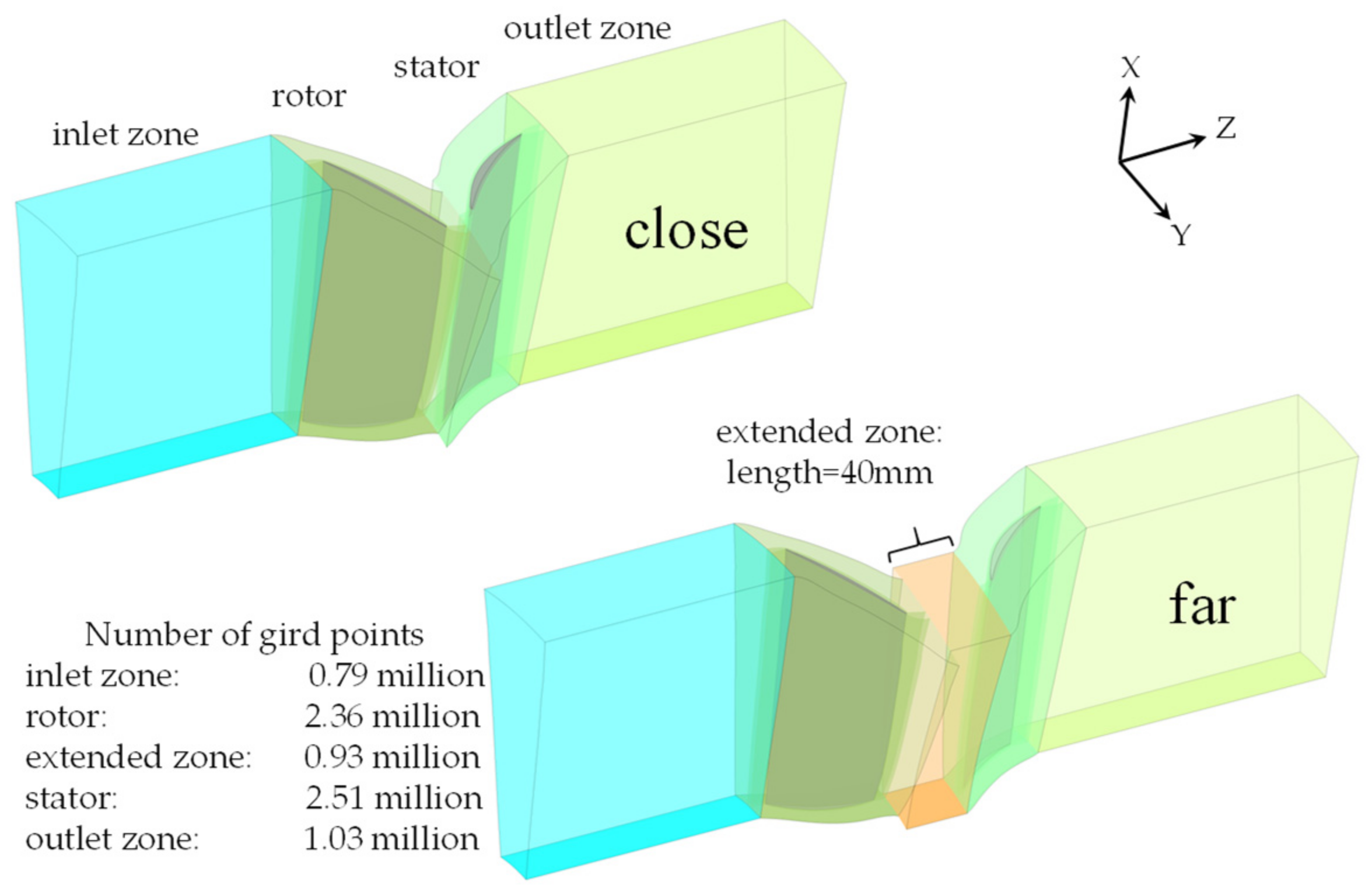
3.1. Mesh Generation

All cases are considered as single-passage computations in this work, and NUMECA/AUTOGRID5 generates the structured mesh. The fluid domain is divided into four subdomains considering a “close” geometry and five subdomains for “far” geometry. The O4H-type mesh is generated at the rotor and stator zones, and an H-type mesh for the other three subdomains. The height of the first layer from the solid surface is set to 1 × 10⁻⁶ m, ensuring that y+ is approximately 1.0. At the chosen three operating conditions, grid independence is validated through five groups of grid settings that are progressively refined in every direction, as shown in Figure 3. The influence of grid number on mass flow is less than one-thousandth and can be ignored. The performance parameters are basically unchanged after the grid number exceeds 2.71 million. To obtain a more accurate unsteady flow, we used the highest density mesh, with the O-type mesh around the blade comprising 36 layers and the radial grid nodes set to 101 and 109 for the rotor and stator, respectively. Additionally, the clearance of rotor and stator involve 25 and 33 nodes, respectively, with the total grid nodes being about 6.69 million for the “close” geometry and 7.62 million for the “far” geometry. The detailed number of grid nodes per fluid subdomain is illustrated in Figure 4.

3.2. Computational Fluid Dynamics Method

The numerical simulations utilize the 3-D unsteady Reynolds-Averaged Navier-Stokes (RANS) solver ANSYS CFX which uses a finite volume method to compute the flow field. The discrete scheme of the convection term is second-order, and thus, a second-order backward Euler is used for the time difference scheme. The shear stress transport turbulence model is also chosen, which is appropriate for unsteady flow research [31,32]. The radial distribution of the stagnation pressure, stagnation temperature, and flow angle is set for the inlet boundary, and the outlet boundary is set to the radial distribution of circumferentially averaged static pressure as indicated by the steady results. The mesh on the periodic boundary is matched and all solid surfaces are adiabatic and non-slip. Every physical time step that includes five iterations is set to 1% of the time in which the rotor rotated by one pitch. All unsteady cases started from their respective steady cases. After computing for about four revolutions, the periodic flow is obtained, and then all the required data is collected within another 20 pitches.

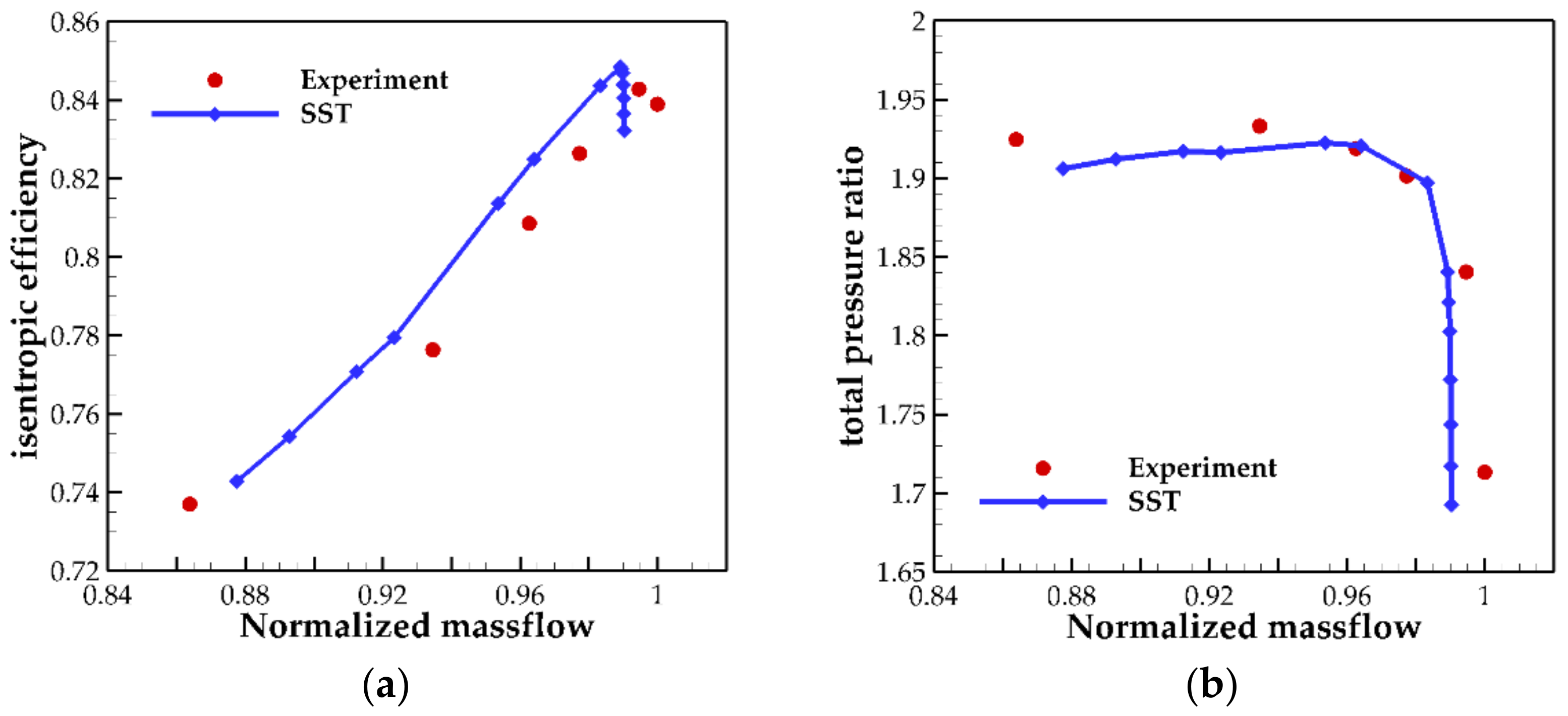
3.3. Validations of Computational Fluid Dynamics Method
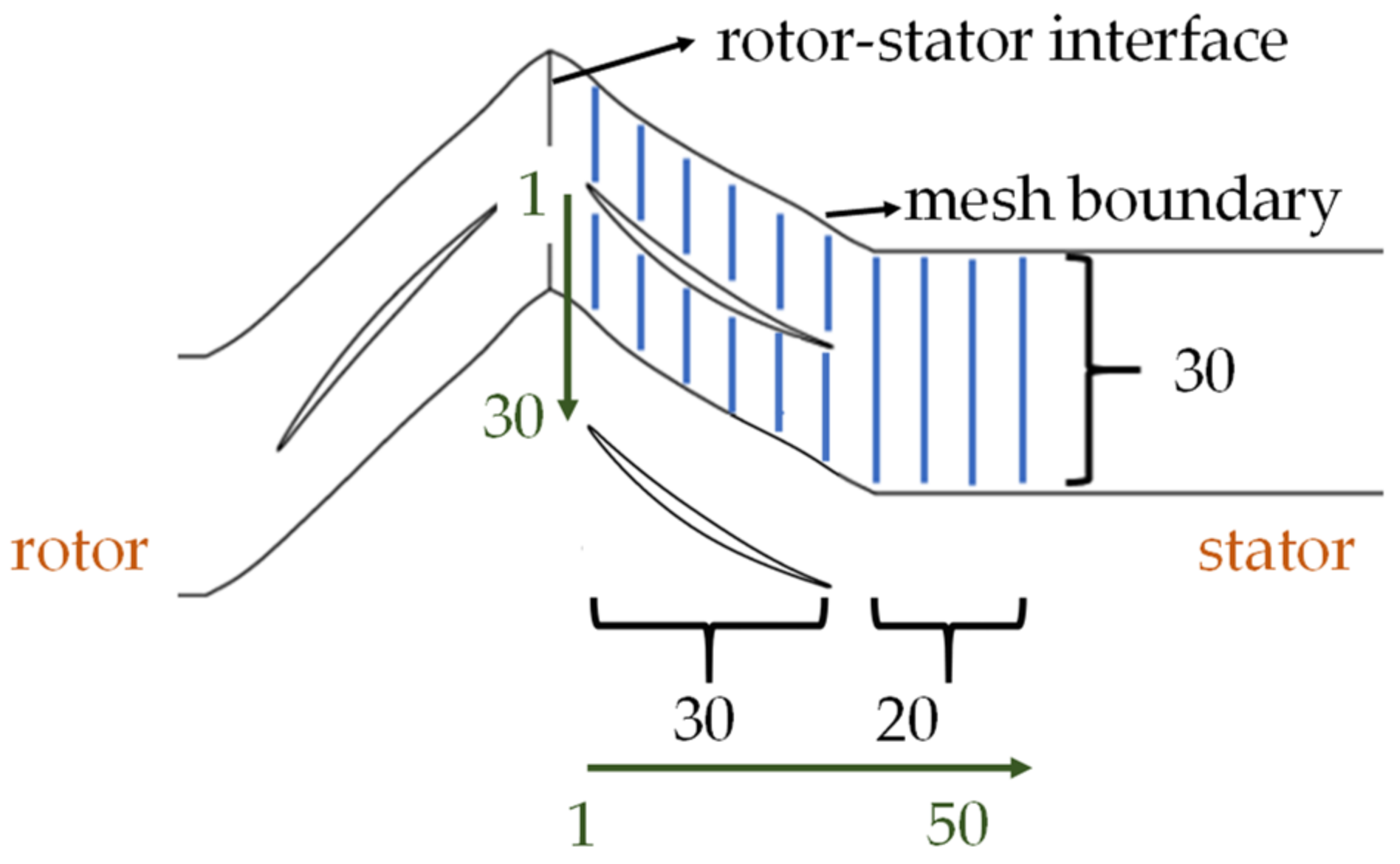
We validate the numerical method on the transonic compressor Stage 35, designed by NASA Glenn [33], for its detailed design and experimental data. The height of the first layer from the solid surface is set to 5 × 10⁻⁷ m to ensure that y+ is approximately 1.0 and the total grid nodes are 6.07 million. Figure 5 compares the calculated results and the experimental data, revealing that the mass flow near the stall is slightly higher than the experimental value, and the choke mass flow is slightly lower than the experimental value. The numerical efficiency characteristic is estimated to be a little higher, and the pressure ratio near the design point is in excellent agreement with experimental values. Overall, the computational fluid dynamics method adopted meets the numerical simulation accuracy required by the research.

3.4. Monitor Scheme

We set the monitor points on a stream surface with a constant radius to receive time-resolved data, as illustrated in Figure 6. The primary monitor points are set in the stator and one-third of the axial chord after the stator. Thirty points are evenly distributed in the circumferential direction from the suction side of one blade to the pressure side of the adjacent blade. Meanwhile, the monitor points that cross the mesh boundary are transformed to the inside of the mesh boundary. In the axial direction, 30 uniform monitor points from the LE to the TE are located, and 20 points have the same spacing as the fore points set after the TE. The radial direction is from the 0.8 span to the 0.99 span, and the spacing between adjacent monitor sections is 0.01 span. There are 20*50*30 monitor points for the specific transient flow analysis, and for other time-resolved data acquisition like velocity distribution in the wake region, the monitor points are set by adopting the above method.

3.5. Data Processing Method

To explore the effect of unsteady interaction on performance, we calculate the time-averaged performance, which is different from the steady and transient performances. Considering the inconsistent results during the time-averaged value calculation per performance parameter, we calculate the mass-averaged value of the basic parameters in the corresponding section to obtain the time-averaged parameters. Finally, the performance parameters are calculated, with the time-averaged efficiency and total pressure loss coefficient defined as:
η ¯ = p o u t * ¯ / p i n * ¯ k 1 k 1 T o u t * ¯ / T i n * ¯ 1
ω ¯ = p i n * ¯ p o u t * ¯ p i n * ¯ p i n ¯

4. Results and Discussions

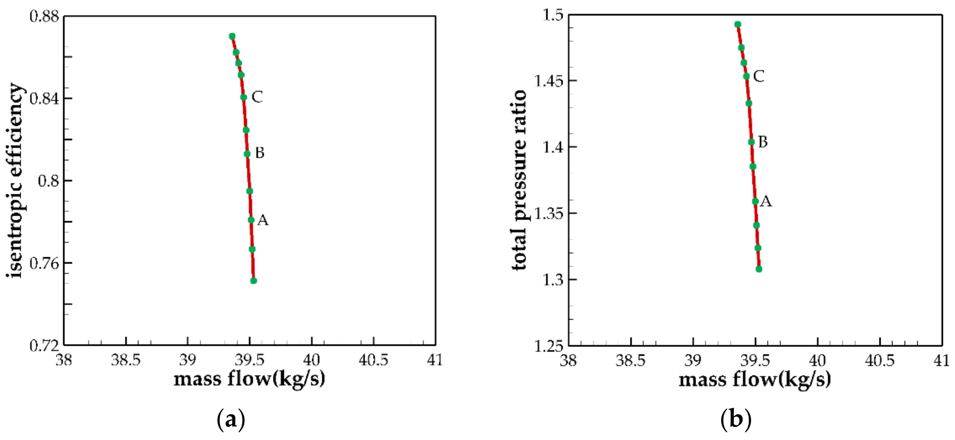
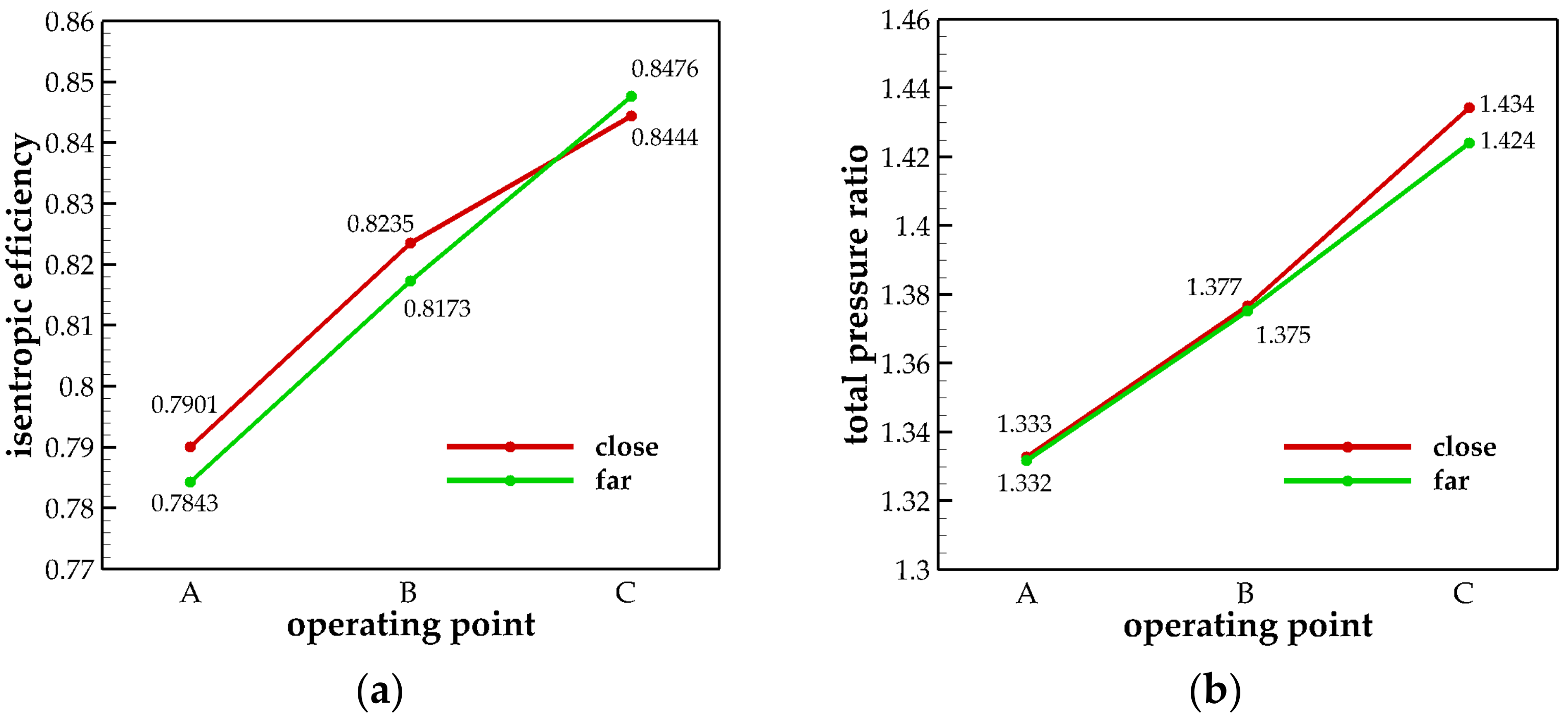
4.1. Performance Analysis

Figure 7 illustrates the transient efficiency in a 20-blade passing period (BPP), reflecting the periodic law of compressor flow. The transient efficiency of all cases except close_C periodically fluctuates with the period of one BPP, while the transient efficiency fluctuation period of close_C is 4 BPP. Thus, some flow structure is dominant in the performance change caused by rotor-stator interaction, with its fluctuation frequency equal to 0.25 blade passing frequency (BPF). Considering the axial spacing from close to far, the transient efficiency decreases at A and B but increases at C. Thus, the flow structure mentioned above is harmful to performance. Figure 8 compares the time-averaged performance between two-axial spacing. The total pressure ratio changes little at A and B, and 0.6 points from close to far almost decline the time-averaged efficiency. At high load conditions, the total pressure ratio decreases by 0.01, but time-averaged efficiency increases by 0.32 points from close to far due to the change of the unsteady interaction characteristics.
Zlatinov [34] et al. used irreversible entropy generation to analyze loss in turbomachinery. Accordingly, Tiralap et al. [32] developed a nondimensional loss coefficient, namely efficiency deficit, as defined in Equation (3), which effectively locates the axial range where performance changes most:
ξ = 1 η = W ˙ l o s t H ˙ s t a g e   = T 0 , s S ˙ g e n e r a t i o n H ˙ s t a g e
Figure 9 illustrates the development of ξ from rotor TE to the outlet, presenting the measurement station setting, which is appropriate due to the non-vertical edge. The loss generation trend for A and B operating conditions is the same. For the same operating condition with different axial spacing, the loss generated by the upstream rotor is almost the same, and at the front of the axial spacing, the loss generation rate of the “far” case is higher, before declining gradually before the stator. Overall, the loss generation rate in each stage is independent of operating conditions, regardless of the axial spacing.
For operating condition C, the loss generated by the upstream rotor of “close” is lower than that of “far”, but the loss has a sharp rise in stator while the loss in the spacing is smaller than that of the other two conditions. Compared with the other two operating conditions, the loss decay rate of far_C is lower in spacing but higher in the stator.
The overall loss is further decomposed into four parts, as depicted in Figure 10. In the compressor stage, the rotor loss is the bulk of the total loss, and the loss generation after the rotor is up to one-third of the total loss as in close_C. The loss difference at the rotor and after the stator is almost negligible at both points A and B; the stator loss is higher, and the spacing loss is lower. The decrease in efficiency from close to far is due to the decreased spacing loss. When the axial spacing increases, the growth rate of loss in the spacing is greater than the decay rate of loss in the stator. Therefore, it can be established that the closer the axial spacing, the higher the efficiency. According to the spacing from far to close at C, the potential effect of the downstream stator is favorable to the rotor, generating lower loss of about 0.01. Simultaneously, the loss in and after the stator increases sharply by 0.017 and 0.005, respectively, leading to a more significant total loss. In addition, it is worth noting that at A and B, the stator loss decreases as the axial spacing becomes larger, failing to present a total performance benefit from wake recovery.
Figure 11 and Figure 12 illustrate the radial distribution of the time-averaged stator inlet parameters and the total pressure loss coefficient defined by Equation (2). At all operating conditions, the parameters between two spacings tend to approach below the 0.05 span, which is the influence range of the hub leakage flow according to the loss distribution. Although the inlet flow angle is smaller, at every operating condition, the loss generated by the hub leakage flow is higher with increased spacing (Figure 12).
The parameter difference between A and B with either spacing is similar above the 0.3 span, indicating that the main characteristics of the unsteady interaction remain unchanged under these two conditions. From the 0.2 to 0.7 span, the loss of every section decreases as the load increases, regardless of the axial spacing. Meanwhile, the loss reduction of “close” is larger, and as a result, the loss of close_B near the 0.4 span drops to less than that of far_B, as shown in the close-up view 4 of Figure 11. Then the span range where the loss of “close” is lower becomes larger as the load continues to increase (view 5 of Figure 12).
At C, the flow angle of “close” is larger above the 0.7 span and when combined with the sudden increase of loss above the 0.8 span. Moreover, the loss difference between the two spacings below the 0.8 span is not prominent, so the sudden increase of the stator loss is attributed to the change in the flow structure caused by unsteady interaction.

4.2. Hub Leakage Flow
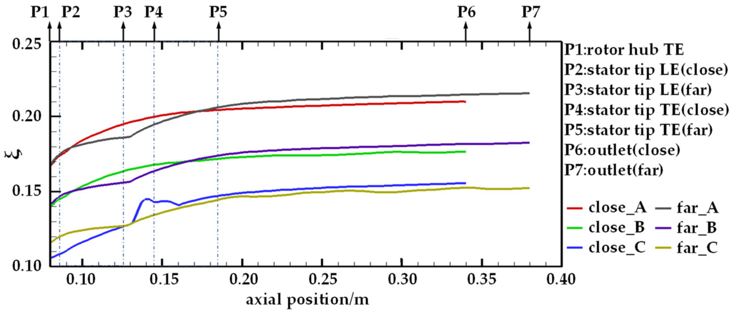
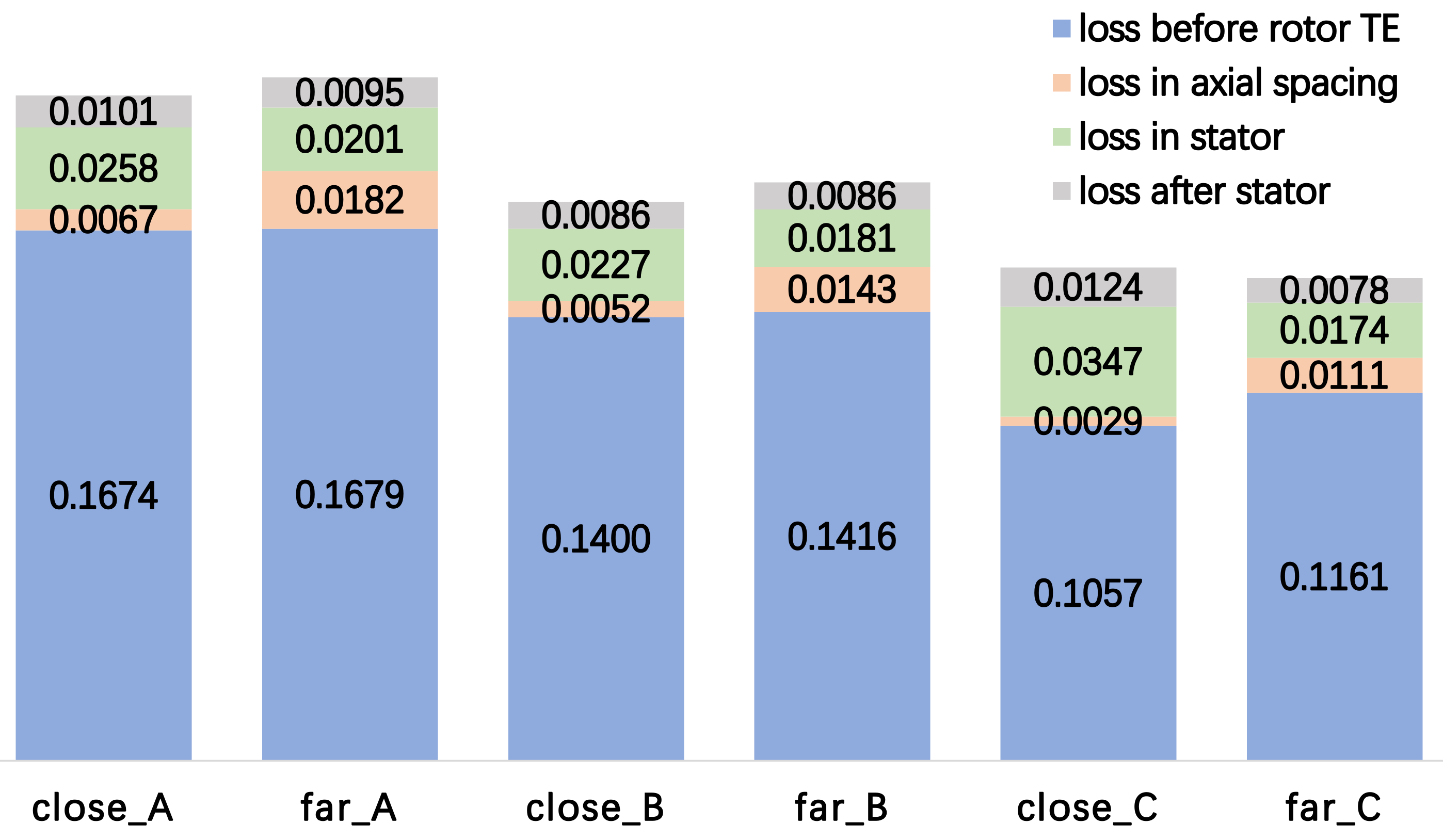
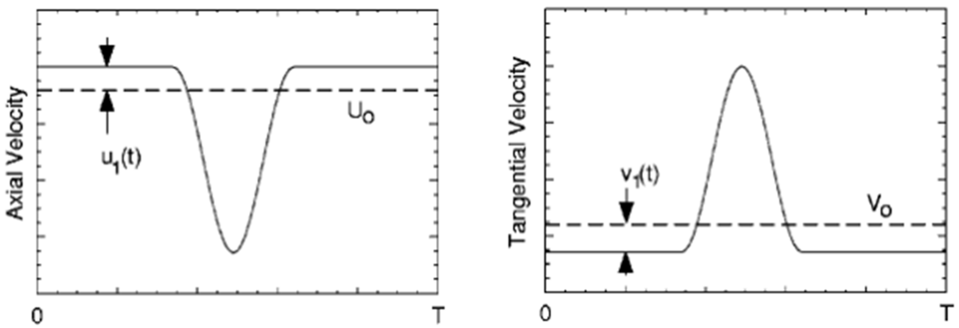
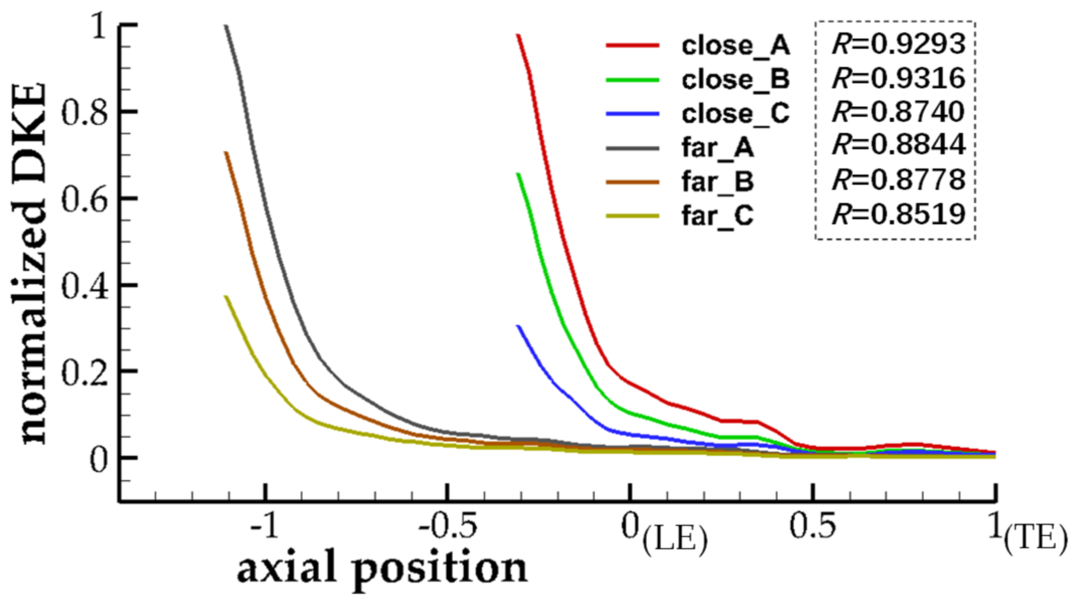
From Figure 11 and Figure 12, we observe that the hub leakage flow’s unloading effect makes the rotor’s loading capacity near the hub not change significantly with overall load increases. Additionally, the loss coefficient of “close” is always lower at every condition than “far”. According to the analysis, the mechanism of this phenomenon under the three operating conditions is consistent. Therefore, this paper considers condition C as an example to explain this. By comparison, we find that the intensity of the leakage vortex is greater at close_C (Figure 13). Indeed, the driving force of hub leakage vortex (HLV) is the pressure difference between the pressure surface (PS) and suction surface (SS) near the hub clearance, and the pressure distribution comparison at the 0.05 span between close_C and far_C is illustrated in Figure 14. The pressure distribution is the same in the fore 10% axial chord. The SS pressure of “close” is higher than that of “far” from 15% to 55% of the axial chord, but the pressure at PS of “close” is lower from 10% to 80% of the axial chord. The corresponding increase is also greater than the previous, indicating that the “close” driving force is lower and the formed HLV is weaker.
Next, we analyze five specific transient moments, t1, t2, t3, t4, and t5 (Figure 15), as well as, at each moment, the wake impacts of PS at positions 0.2, 0.3, 0.4, 0.5, and 0.6 times the axial chord. Figure 15a distinguishes the wake using the Q-criterion and reveals the wake mixing in the axial spacing reduces the vortex structure in the wake section, and the corresponding velocity deficit is also lower in the far_C. Additionally, the deflection angle of the wake passing through the stator passage is very small, which leads to the close chord-wise position of the wake sections on both sides of the blade.
In Figure 15b, the dotted line represents the position of the wake. The flow transport caused by the wake negative jet [35] makes the fluid at the SS flow towards the pressure side, and the transverse transport makes the pressure field along the wake direction consistent. In Figure 15b and Figure 16, when at t1, the slip velocity of the wake is relatively large, and the high-pressure fluid transported to the PS significantly increases the pressure enhancing the pressure rise gradient. However, the high-pressure area near the trailing edge is smaller owing to its lower outlet pressure at close_C. Then at t2, the pressure distribution on the PS is almost the same. At t3, the pressure from 0.2 to 0.55 axial chord at close_C drops, and the pressure drop decreases in the next two moments.
These findings indicate that the pressure at a particular position of the PS depends on the influence of the downstream pressure field and the combined action of wake transport. The wake transport has three factors affecting pressure: (1) wake slip velocity and wake decay that characterizes the fluid transport mass flow along the flow direction, (2) chord-wise load distribution and deflection angle of the wake that decides the pressure of the initial transported fluid, and (3) transverse pressure gradient that influences the pressure variation during the wake transport to the PS. Considering these factors comprehensively, the transport fluid’s pressure is higher than that of the downstream pressure field at t1, and the two functions are balanced at t2. When at t3, the low-pressure fluid transported by the wake has the most apparent effect on the pressure surface. The high pressure of the downstream pressure field has a greater influence on the interaction position of the wake and the PS. Meanwhile, Figure 15 illustrates a reduced slip velocity, increased pressure of the initial transported fluid, and higher pressure in the wake transport path. Thus, the pressure difference at the PS between close_C and far_C decrease gradually from t3 to t5. Finally, close_C has a lower time-averaged driving force near the hub in the entire BPP, generating a weaker HLV.

4.3. Wake Recovery

In the analysis of Section 4.1, we demonstrate that the stator loss near the 0.4 span in the “close” case decreases. The flow angle comparison in view 4 of Figure 11 highlights that the time-averaged flow angle difference at B and C is almost negligible, and the non-transitional boundary layer response affords “close”, giving more loss because of the existing deep wake just before the stator contributes to the loss [13].
As mentioned in the introduction, Adamczyk [8] used the unsteady kinetic energy flux defined in Equation (4) to describe the flow unsteadiness, where u 1 and v 1 represent the axial and tangential velocity, as illustrated in Figure 17. The recovery parameter R is calculated from Equation (5). Van Zante [9] removed the pitch-wise operator A y and solely employed flow data at the mid-pitch, called disturbance kinetic energy(DKE), a method adopted in this paper.
K =   0.5 U 0 A y A t u 1 2 + v 1 2
K i n K o u t   = K i n R
DKE =   0.5 U 0 A t u 1 2 + v 1 2
We set monitoring points in the two-dimensional cylindrical surface of the 0.4 span (Figure 6), which are extended forward of the rotor’s TE so that the last location in the axial direction is the stator’s TE. In total, one point in the circumferential direction at the mid-pitch and twenty-one points, including the LE and the TE in the axial direction, are set in the blade passage to monitor three velocity components. There are ten and thirty for “close” and “far” in the axial spacing, respectively. By analyzing each point’s data, the ratio of radial kinetic energy to the total kinetic energy in the non-near blade surface area of the stator does not exceed 1.5%, revealing that the two-dimensional wake recovery analysis using Equation (6) at the span is practical.
Figure 18 highlights that the axial variation of DKE from the rotor TE to the stator TE, in which DKE is non-dimensionally treated, along with the maximum value and axial position, is normalized with the stator’s axial chord length. The DKE at the rotor TE gradually decreases as the load increases, indicating that the wake’s velocity deficit decreases. To compare the two spacing, the bigger the DKE entering the stator, the greater the value of R. For the cases with a far spacing, the wake’s DKE almost decayed entirely before entering the stator; thus, the stator’s performance is regarded as steady. At the same condition, the difference of R is sorted as B > A > C, but this is inconsistent with the total pressure loss comparison presented in Figure 12. Moreover, the wake decay is caused by wake recovery and dissipation, so we use the integration of turbulence eddy dissipation in a thin cylinder at the 0.4 span (Equation (7)) to quantify dynamic pressure loss. Additionally, we use the vorticity criterion to identify the edge of the boundary layer (Figure 19). Moreover, we define ωpotential (Equation (8)) to characterize potential loss due to non-uniform freestream, highlighting its significance when used as a relative quantity.
ω t = Ω ρ ε d Ω / 1 2 m ˙ i n U i n 2
ω p o t e n t i a l = DKE in / 1 2 U i n 3
The interface is used as the starting position in the detailed loss analysis. At every condition, ωpotential of “far” is more extensive, and the difference is 0.0014, 0.0006, and 0.0010, respectively, which is small enough to be ignored, and thus the detailed loss comparison is reasonable. As illustrated in Figure 19, the total loss of “far” is more extensive in every case where the loss in the spacing contributes the most. As load increases, the proportion of the loss in the spacing decreases, although the increased stator load will aggravate the wake mixing in the gap, showing that the wake’s reduced velocity deficit has the greatest impact on the loss in the spacing. The loss in the boundary layer between the two spacing is not apparent under the same conditions, indicating that the interaction between wake and boundary layer has a minor effect on the loss. The DKE at the stator LE of “far” can be almost ignored, and the loss difference in the freestream can be attributed to the mixing loss in the wake attenuation process. The effect of wake stretch reflects the benefit of the wake recovery on R and the inlet wake velocity deficit. With the load increase, the first factor increases, the second decreases, and the wake mixing loss difference between the two spacing become smaller. Hence, combined with Figure 12, we conclude that the small wake stretch effect caused by negative incidence and large incoming DKE makes the total pressure loss coefficient of “close” greater at A. Then, the proportion of viscous mixing in the attenuation of DKE decreases, and the wake recovery benefit increases. So, the wake recovery effect dominates instead of the wake mixing in the stator, reducing the total pressure loss coefficient of “close”.

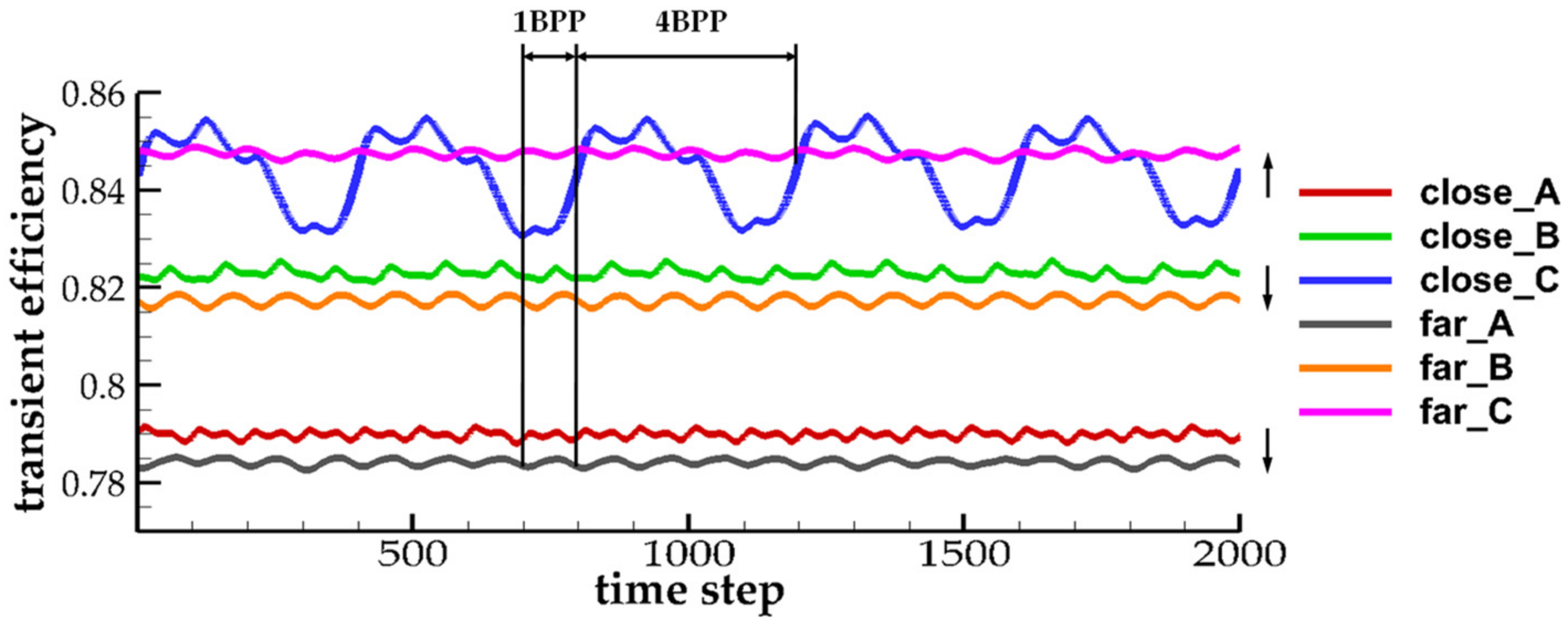
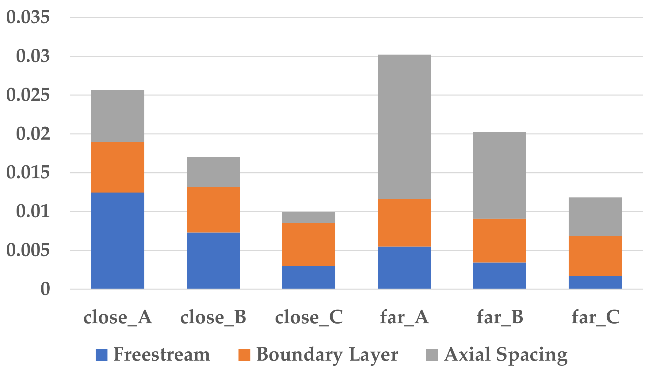
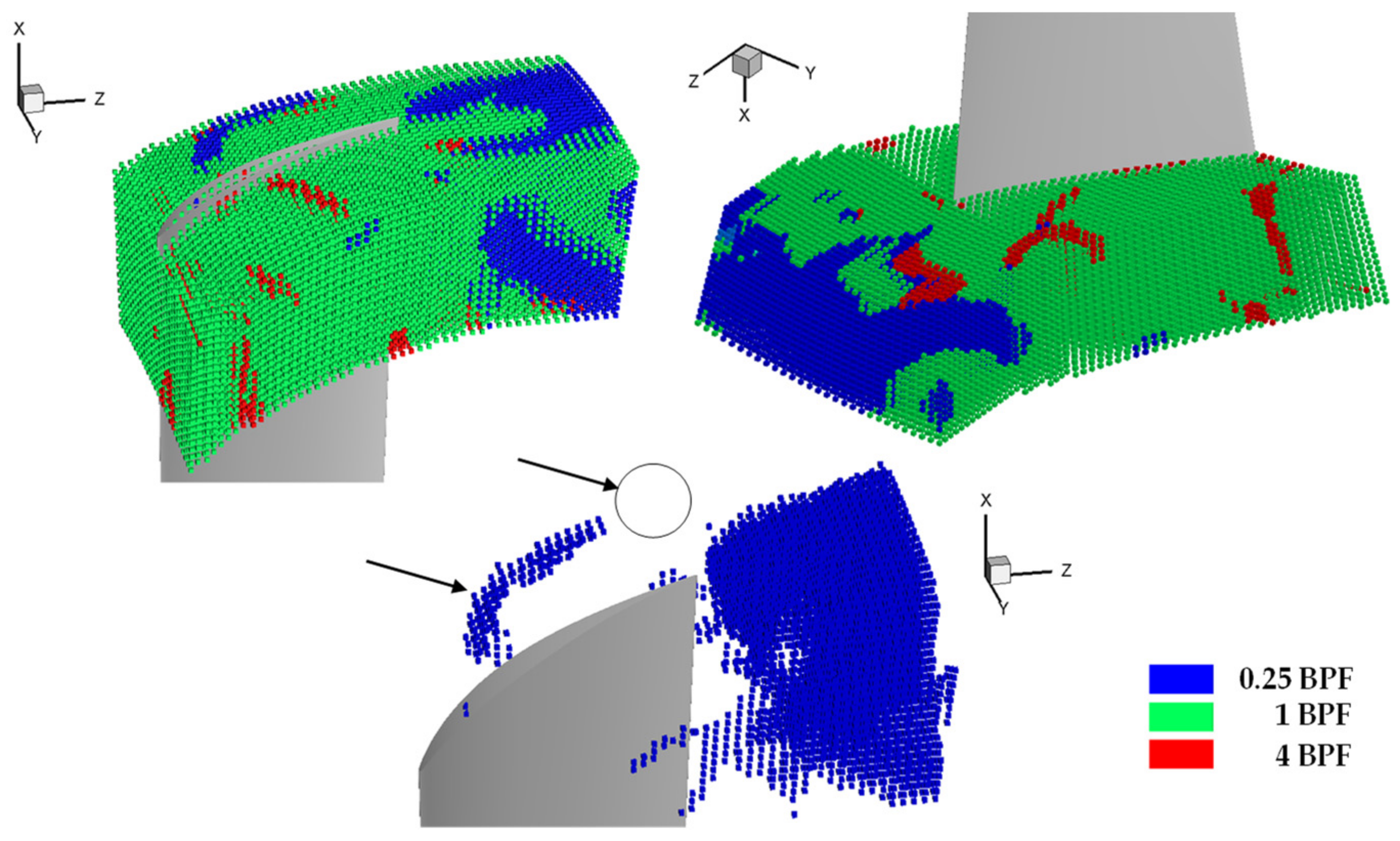
4.4. Performance Fluctuation Analysis

Figure 7 reveals that the efficiency of close_C fluctuates at 0.25 BPF. The simple flow analysis highlights that three-dimensional corner separation occurs in close_C, but a minor separation occurs in far_C near the shroud. The wake is transported in the form of a negative jet, weakening the attached ability of the boundary layer of the suction surface. A high enough load and deep wake with great slip velocity work together to determine the occurrence of separation, and therefore, corner separation occurs in close_C. This paper focuses on analyzing the reasons for performance fluctuation frequency. Since the major loss generated is above the 0.80 span, we use the monitoring scheme described in Section 3.4 to collect the total pressure data of close_C.
Moreover, we propose a dominant frequency screening method based on Fast Fourier Transform (FFT). FFT is used to analyze the data of every monitor point, and then we obtained the frequency corresponding to the maximum amplitude called dominant frequency. Figure 20 highlights that only three frequencies as dominant frequencies exist in the flow field, and they are 0.25, 1, and 4 times the BPF. The dominant frequency of four BPF is scattered in several isolated locations, and the effect on the entire flow is not apparent. The dominant frequency of one BPF occupies most positions inside the stator passage, but its dominant positions gradually decrease after the TE. The positions dominated by 0.25 BPF are very few in the stator passage, and one of them coincides with the tip separation boundary. However, this area discontinues before it develops to the TE. After the TE, the region dominated by 0.25 BPF gradually develops, becomes larger, and the frequency dominates the entire flow.
We performed a Dimensionless Power Spectral Density (PSD) analysis on all data (Figure 21). At the same time, the ratio of the dominant frequency power to the total power of all frequencies is analyzed (Figure 22). Although the analysis ignores the phase relationship between every frequency component, it is dominant as long as the power ratio of the dominant frequency exceeds 0.5, even when all other frequencies are in the reverse phase.
The zones whose PSD of the dominant frequency is relatively large are the zones before the TE at the tip and the wake region at the tip (Figure 21(1)), while the dominant frequency of the second one is 0.25 BPF. Figure 21(2) shows that the PSD of 0.25 BPF frequency is very low in the stator passage and very high in the wake region. These two reasons, combined with the discontinuity of the dominant frequency of 0.25 BPF at the separation boundary, indicate that the excitation of the separation boundary does not generate the dominant frequency of 0.25 BPF in the wake region. The wake’s self-excited oscillation is why the wake oscillates at 0.25 BPF, and the region dominated by 0.25 BPF gradually expands to the entire spanwise range.
At the LE, the one BPF frequency occupies a dominant position, and either its PSD is relatively large, or the power ratio is close to one. Thus, the 0.25 BPF frequency is not generated by the excitation of the flow that contains the frequency component from the upstream rotor. The one BPF flow covers the initial position of the separation boundary with a much higher PSD and power ratio. Therefore, the oscillation of the separation boundary with the dominant frequency of 0.25 BPF is caused by wake interaction. In Figure 21(2), the wake and mid-pitch regions have a 0.25 BPF frequency with high power at the outlet. The flow formed by the backward development of the separation boundary after interacting with the wake (Figure 21 and Figure 22) can be verified by the evolution process in four BPP at the 0.95 span (Figure 23).
The above analysis reveals that the wake oscillation with a dominant frequency of 0.25 BPF makes the separation boundary oscillate with the same frequency at the tip, and the combination of the two regions makes the performance fluctuate at this frequency.

5. Conclusions

This paper performs three-dimensional URANS calculations in a transonic compressor stage with an equal radius flow path to explore the influence of the rotor-stator spacing and variable operating conditions on performance. Detailed performance analysis and the corresponding flow mechanism of two-axial spacing cases at three operating conditions are investigated.
For all conditions, the HLV loss in “close” is low, the fluid transported by wake reaches the PS, and the impact of the downstream pressure field jointly affects the local pressure. In homogenizing the transverse pressure distribution, the wake’s transport reduces the pressure on the PS from 10% to 80% of the axial chord, reducing the loss from leakage. Regardless of the rotor or stator, the stage performance near the end wall can be improved by adequately enhancing the upstream blade wake.
Wake recovery has a minor contribution to the overall performance of this compressor. In the span range near the 0.4 span, it plays a positive role with non-negative incidence when the axial spacing is close. The sufficient, incompletely mixed wake flowing into the stator is stretched, which highlights the role of wake recovery by reducing mixing loss. If the corner separation does not occur, more elements will benefit from wake recovery until the boundary layer separation becomes very large.
At low and nominal load conditions, the stage efficiency of “close” is higher, and the loss in axial spacing mainly contributes to the change of about 0.6 points of stage efficiency. At high load conditions, the stage efficiency of “close” is lower by 0.3 points, because the deep wake makes corner separation occur near the shroud. The stator wake near the shroud oscillates with a frequency of 0.25 BPF which gives the efficiency the same fluctuation frequency.

Author Contributions

Conceptualization, H.N.; Data curation, H.N.; Formal analysis, H.N.; Funding acquisition, J.C.; Investigation, H.N.; Methodology, H.N.; Project administration, J.C.; Resources, J.C.; Software, H.N.; Supervision, J.C.; Validation, H.N.; Visualization, H.N.; Writing—original draft, H.N.; Writing—review & editing, H.N. and H.X. All authors have read and agreed to the published version of the manuscript.

Funding

This research was funded by National Science and Technology Major Project, China (J2019-II-0005-0025).

Institutional Review Board Statement

Not applicable.

Informed Consent Statement

Not applicable.

Data Availability Statement

All the data produced in this study is contained in the manuscript text.

Acknowledgments

The authors would like to thank the guidance and kind advice of Zhi-yuan CAO and to express their gratitude to EditSprings (https://www.editsprings.cn, accessed on 3 June 2022) for the expert linguistic services provided.

Conflicts of Interest

The authors declare no conflict of interest.

Abbreviations

Nomenclature
η ¯ time-averaged isentropic efficiency
p * ¯ time-averaged total pressure
p ¯ time-averaged pressure
T * ¯ time-averaged total temperature
ω ¯ time-averaged total pressure loss coefficient
kspecific heat ratio
W ˙ l o s t loss work
H ˙ s t a g e enthalpy change rate across stage
T 0 , s stagnation temperature
S ˙ g e n e r a t i o n entropy generation rate
ξnondimensional loss coefficient
U 0 ,   V 0 axial and tangential time-averaged velocity
u 1 ,   v 1 axial and tangential velocity
A y pitch-wise average operator
A t time average operator
Kunsteady kinetic energy flux
Rwake recovery parameter
ρ density
ε turbulence eddy dissipation
m ˙ mass flow rate
U inlet velocity
ω t dynamic pressure loss
ω p o t e n t i a l potential loss
Subscripts
ininlet
outoutlet
Ω integral space

References

  1. Chriss, R.M.; Copenhaver, W.W.; Gorrell, S.E. The Effects of Blade-Row Spacing on the Flow Capacity of a Transonic Rotor. In Proceedings of the ASME 1999 International Gas Turbine and Aeroengine Congress and Exhibition, Indianapolis, IN, USA, 7–10 June 1999. [Google Scholar]
  2. Milidonis, K.; Semlitsch, B.; Hynes, T. Effect of Clocking on Compressor Noise Generation. AIAA J. 2018, 56, 4225–4231. [Google Scholar] [CrossRef]
  3. Hellmich, B.; Seume, R.J. Causes of Acoustic Resonance in a High-Speed Axial Compressor. ASME J. Turbomach. 2008, 130, 31003. [Google Scholar] [CrossRef]
  4. Wo, A.M.; Chung, M.H.; Gorrell, S.E.; Lee, S.F. Wake Vorticity Decay and Blade Response in an Axial Compressor with Varying Axial Gap. In Proceedings of the ASME 1999 International Gas Turbine and Aeroengine Congress and Exhibition, Indianapolis, IN, USA, 7–10 June 1999. [Google Scholar]
  5. Smith, L.H. Casing Boundary Layers in Multistage Axial-Flow Compressors. In Flow Research in Blading; Dzung, L.S., Ed.; Elsevier: Amsterdam, The Netherlands, 1970; pp. 275–304. [Google Scholar]
  6. Smith, L.H. Wake Dispersion in Turbomachines. ASME J. Basic Eng. 1996, 88, 688–690. [Google Scholar] [CrossRef]
  7. Smith, L.H. Wake Ingestion Propulsion Benefit. J. Propuls. Power 1993, 9, 74–82. [Google Scholar] [CrossRef]
  8. Adamczyk, J.J. Wake mixing in axial flow compressors. In Proceedings of the ASME 1996 International Gas Turbine and Aeroengine Congress and Exhibition, Birmingham, UK, 10–13 June 1996. [Google Scholar]
  9. Van Zante, D.E.; Adamczyk, J.J.; Strazisar, A.J.; Okiishi, T.H. Wake Recovery Performance Benefit in a High-Speed Axial Compressor. ASME J. Turbomach. 2002, 124, 275–284. [Google Scholar] [CrossRef]
  10. Van de Wall, A.G.; Kadambi, J.R.; Adamczyk, J.J. A Transport Model for the Deterministic Stresses Associated with Turbomachinery Blade Row Interactions. ASME J. Turbomach. 2000, 122, 593–603. [Google Scholar] [CrossRef]
  11. Pallot, G.; Kato, D.; Kanameda, W.; Ohta, Y. Effect of Incoming Wakes on the Stator Performance in a Single-Stage Low Speed Axial Flow Compressor Operating at Design and Near Stall Conditions. In Proceedings of the ASME Turbo Expo 2016: Turbomachinery Technical Conference and Exposition, Seoul, Korea, 13–17 June 2016. [Google Scholar]
  12. Deregel, P.; Tan, C.S. Impact of Rotor Wakes on Steady-State Axial Compressor Performance. In Proceedings of the ASME 1996 International Gas Turbine and Aeroengine Congress and Exhibition, Birmingham, UK, 10–13 June 1996. [Google Scholar]
  13. Valkov, T.V.; Tan, C.S. Effect of Upstream Rotor Vortical Disturbances on the Time-Average Performance of Axial Compressor Stators: Part 1—Framework of Technical Approach and Wake-Stator Blade Interactions. In Proceedings of the ASME 1998 International Gas Turbine and Aeroengine Congress and Exhibition, Stockholm, Sweden, 2–5 June 1998. [Google Scholar]
  14. Valkov, T.V.; Tan, C.S. Effect of Upstream Rotor Vortical Disturbances on the Time-Average Performance of Axial Compressor Stators: Part 2—Rotor Tip Vortex/Streamwise Vortex-Stator Blade Interactions. In Proceedings of the ASME 1998 International Gas Turbine and Aeroengine Congress and Exhibition, Stockholm, Sweden, 2–5 June 1998. [Google Scholar]
  15. Hah, C. Impact of Wake Dispersion on Axial Compressor Performance. In Proceedings of the ASME Turbo Expo 2017: Turbomachinery Technical Conference and Exposition, Charlotte, NC, USA, 26–30 June 2017. [Google Scholar]
  16. Przytarski, P.J.; Wheeler, A.P.S. The Effect of Gapping on Compressor Performance. ASME J. Turbomach. 2020, 142, 121006. [Google Scholar] [CrossRef]
  17. Zachcial, A.; Nürnberger, D. A Numerical Study on the Influence of Vane-Blade Spacing on a Compressor Stage at Sub- and Transonic Operating Conditions. In Proceedings of the ASME Turbo Expo 2003, Collocated with the 2003 International Joint Power Generation Conference, Atlanta, GE, USA, 16–19 June 2003. [Google Scholar]
  18. Gorrell, S.E.; Car, D.; Puterbaugh, S.L.; Estevadeordal, J.; Okiishi, T.H. An Investigation of Wake-Shock Interactions in a Transonic Compressor with Digital Particle Image Velocimetry and Time-Accurate Computational Fluid Dynamics. ASME J. Turbomach. 2006, 128, 616–626. [Google Scholar] [CrossRef]
  19. Clark, K.P.; Gorrell, S.E. Analysis and Prediction of Shock-Induced Vortex Circulation in Transonic Compressors. ASME J. Turbomach. 2015, 137, 121007. [Google Scholar] [CrossRef]
  20. Estevadeordal, J.; Gorrell, S.E.; Copenhaver, W.W. PIV Study of Wake–Rotor Interactions in a Transonic Compressor at Various Operating Conditions. J. Propuls. Power 2007, 23, 235–242. [Google Scholar] [CrossRef]
  21. Gorrell, S.E.; Okiishi, T.H.; Copenhaver, W.W. Stator-Rotor Interactions in a Transonic Compressor—Part 1: Effect of Blade-Row Spacing on Performance. ASME J. Turbomach. 2003, 125, 328–335. [Google Scholar] [CrossRef]
  22. List, M.G.; Gorrell, S.E.; Turner, M.G. Investigation of Loss Generation in an Embedded Transonic Fan Stage at Several Gaps Using High-Fidelity, Time-Accurate Computational Fluid Dynamics. ASME J. Turbomach. 2010, 132, 11014. [Google Scholar] [CrossRef]
  23. Poensgen, C.; Gallus, H.E. Three-Dimensional Wake Decay Inside of a Compressor Cascade and Its Influence on the Downstream Unsteady Flow Field: Part II—Unsteady Flow Field Downstream of the Stator. J. Turbomach. 1991, 113, 190–197. [Google Scholar] [CrossRef]
  24. Sirakov, B.T.; Tan, C.S. Effect of Unsteady Stator Wake—Rotor Double-Leakage Tip Clearance Flow Interaction on Time-Average Compressor Performance. ASME J. Turbomach. 2003, 125, 465–474. [Google Scholar] [CrossRef]
  25. Nolan, S.P.R.; Botros, B.B.; Tan, C.S.; Adamczyk, J.J.; Greitzer, E.M.; Gorrell, S.E. Effects of Upstream Wake Phasing on Transonic Axial Compressor Performance. ASME J. Turbomach. 2011, 133, 21010. [Google Scholar] [CrossRef]
  26. Mailach, R.; Lehmann, I.; Vogeler, K. Periodical Unsteady Flow Within a Rotor Blade Row of an Axial Compressor—Part I: Flow Field at Midspan. ASME J. Turbomach. 2008, 130, 41004. [Google Scholar] [CrossRef]
  27. Lange, M.; Rolfes, M.; Mailach, R.; Schrapp, H. Periodic Unsteady Tip Clearance Vortex Development in a Low-Speed Axial Research Compressor at Different Tip Clearances. ASME J. Turbomach. 2018, 140, 31005. [Google Scholar] [CrossRef]
  28. Krug, A.; Busse, P.; Vogeler, K. Experimental Investigation into the Effects of the Steady Wake-Tip Clearance Vortex Interaction in a Compressor Cascade. ASME J. Turbomach. 2015, 137, 61006. [Google Scholar] [CrossRef]
  29. Layachi, M.Y.; Bölcs, A. Effect of the Axial Spacing Between Rotor and Stator with Regard to the Indexing in an Axial Compressor. In Proceedings of the ASME Turbo Expo 2001: Power for Land, Sea, and Air. Volume 1: Aircraft Engine; Marine; Turbomachinery; Microturbines and Small Turbomachinery, New Orleans, LA, USA, 4–7 June 2001. [Google Scholar]
  30. Liu, B.; Qiu, Y.; An, G.; Yu, X. Experimental Investigation of the Flow Mechanisms and the Performance Change of a Highly Loaded Axial Compressor Stage with/without Stator Hub Clearance. Appl. Sci. 2019, 9, 5134. [Google Scholar] [CrossRef] [Green Version]
  31. Cornelius, C.; Biesinger, T.; Galpin, P.; Braune, A. Experimental and Computational Analysis of a Multistage Axial Compressor Including Stall Prediction by Steady and Transient CFD Methods. ASME J. Turbomach. 2014, 136, 61013. [Google Scholar] [CrossRef]
  32. Tiralap, A.; Tan, C.S.; Donahoo, E.; Montgomery, M.; Cornelius, C. Effects of Rotor Tip Blade Loading Variation on Compressor Stage Performance. ASME J. Turbomach. 2017, 139, 51006. [Google Scholar] [CrossRef] [Green Version]
  33. Reid, L.; Moore, R. Performance of Single-Stage Axial-Flow Transonic Compressor with Rotor and Stator Aspect Ratios of 1.19 and 1.26, Respectively, and with Design Pressure Ratio of 1.82; Technical Publication NASA-TP-1338; NASA: Washington, DC, USA, 1978.
  34. Zlatinov, M.B.; Tan, C.S.; Montgomery, M.; Islam, T.; Harris, M. Turbine Hub and Shroud Sealing Flow Loss Mechanisms.ASME. J. Turbomach. 2012, 134, 61027. [Google Scholar] [CrossRef]
  35. Meyer, R.X. The Effect of Wakes on the Transient Pressure and Velocity Distributions in Turbomachines. Trans. ASME. 1958, 80, 1544–1551. [Google Scholar] [CrossRef]
Figure 1. The meridian view of the research compressor.
Applsci 12 06932 g001
Figure 2. Overall performance of the research compressor. (a) Efficiency Characteristic. (b) Total Pressure Ratio Characteristic.
Applsci 12 06932 g002
Figure 3. Validation of grid independence of the research compressor. (a) Isentropic Efficiency; (b) Total Pressure Ratio.
Applsci 12 06932 g003
Figure 4. Mesh of the research compressor.
Applsci 12 06932 g004
Figure 5. Performance comparison of the transonic compressor Stage 35. (a) Isentropic Efficiency. (b) Total Pressure Ratio.
Applsci 12 06932 g005
Figure 6. The setting of monitoring points.
Applsci 12 06932 g006
Figure 7. Transient efficiency of the research compressor.
Applsci 12 06932 g007
Figure 8. Time-averaged performance of the research compressor. (a) Isentropic Efficiency. (b) Total Pressure Ratio.
Applsci 12 06932 g008
Figure 9. Loss generation from rotor TE to the outlet.
Applsci 12 06932 g009
Figure 10. Time-averaged loss decomposition.
Applsci 12 06932 g010
Figure 11. Radial distribution of the time-averaged stator inlet parameters.
Applsci 12 06932 g011
Figure 12. Radial distribution of the time-averaged stator loss coefficient.
Applsci 12 06932 g012
Figure 13. Time-averaged entropy contour near the hub.
Applsci 12 06932 g013
Figure 14. Time-averaged pressure distribution of the 0.05 span at C condition.
Applsci 12 06932 g014
Figure 15. Flow field comparison at five time-steps. (a) Q; (b) Pressure.
Applsci 12 06932 g015
Figure 16. Transient pressure distribution of the 0.05 span at C condition.
Applsci 12 06932 g016
Figure 17. Velocity components of disturbance kinetic energy.
Applsci 12 06932 g017
Figure 18. Comparison of the DKE decay.
Applsci 12 06932 g018
Figure 19. Turbulence eddy dissipation in freestream and boundary layer.
Applsci 12 06932 g019
Figure 20. Dominant frequency analysis of close_C.
Applsci 12 06932 g020
Figure 21. PSD analysis of close_C.
Applsci 12 06932 g021
Figure 22. Power ratio analysis of close_C.
Applsci 12 06932 g022
Figure 23. Mach number at the 0.95 span of close_C.
Applsci 12 06932 g023
Table 1. Geometric parameters of the research compressor.
ParametersValue
Hub-tip ratio0.416
Rotational speed/rpm15,000
Rotor aspect ratio2.242
Stator aspect ratio2.598
Rotor solidity(midspan)1.364
Stator solidity(midspan)1.177
Rotor blade count25
Stator blade count25
Rotor tip clearance0.18% span
Stator hub clearance0.90% span
Table 2. The steady performance of two geometry at three operating points.
CaseMass Flow
(KG/S)
Isentropic
Efficiency
Total Pressure Ratio
close_A39.510.78091.341
close_B39.480.81301.385
close_C39.450.84051.433
far_A39.530.77911.333
far_B39.480.81411.376
far_C39.400.84221.436
Publisher’s Note: MDPI stays neutral with regard to jurisdictional claims in published maps and institutional affiliations.

