GPU-Accelerated Target Strength Prediction Based on Multiresolution Shooting and Bouncing Ray Method

Abstract

The application of the traditional planar acoustics method is limited due to the low accuracy when computing the echo characteristics of underwater targets. Based on the concept of the shooting and bouncing ray which considers multiple reflections on the basic of the geometrics optics principle, this paper presents a more efficient GPU-accelerated multiresolution grid algorithm in the shooting and bouncing ray method (SBR) to quickly predict the target strength value of complex underwater targets. The procedure of the virtual aperture plane generation, ray tracing, scattered sound field integral and subdividing the divergent ray tubes are all implemented on the GPU. Particularly, stackless KD-tree traversal is adopted to effectively improve the ray-tracing efficiency. Experiments on the rigid sphere, cylinder and corner reflector model verify the accuracy of GPU-based multiresolution SBR. Besides, the GPU-based SBR is more than 750 times faster than the CPU version because of its tremendous computing capability. Further, the proposed accelerated GPU-based multiresolution SBR improves runtime performance at least 2.4 times that of the single resolution GPU-based SBR.

1. Introduction

Sonar target strength (TS) [1,2] is an important parameter to describe the echo characteristics of underwater targets. At present, some methods are available to predict the echo intensity of the targets, such as the physical acoustic method [3,4], T matrix method [5] and graphical acoustics computing method [6]. Particularly, the planar element method (PEM) [7,8,9], which uses a set of planar elements to approximate the target surface and superimposes the scattered sound field of each planar element to obtain an approximate value of the total scattered sound field. LIU et al. [10] proposed to apply the Gordon integral algorithm to the PEM in order to improve the stability and rapidity of integral computation.

The shooting and bouncing ray (SBR) [11,12] is a mature and versatile algorithm of the high-frequency method, which is always used to predict the radar cross section (RCS) [13,14] of electrically large and complex targets. The SBR algorithm considers multiple reflections on the basis of geometrics optics (GO) between target geometrics; ray tracing is used to obtain the intersection positions between the incident ray and the triangular patch and then calculate the scattered field according to the physical optics (PO) principle. Tao, Yu-Bo et al. [15] presented a KD-tree to reduce the times that are required to trace each ray tube. Sungha Suk et al. [16] adopted the multiresolution grid algorithm to reduce the total number of ray tubes that participated in calculating the field integral. Bang, J.-K. et al. [17] used the space-division algorithm and the multiresolution grid algorithm to speed up ray tracing in RCS prediction.

The graphics processing unit (GPU) has developed ultra-high computing power in recent years. It is precisely by virtue of the GPU’s super floating-point computing power that the Tianhe 1A supercomputer won the TOP500 championship in 2010, and the Titan supercomputer won the TOP500 championship in 2012. NVIDIA released Maxwell, Pascal, Volta, and Turing architectures in 2015, 2016, 2017, and 2018, respectively. The latest Turing architecture enables ray tracing through hybrid rendering, and the new RT Core processes rays 25 times faster than Pascal. What’s more, the compute unified device architecture (CUDA) is a hardware system introduced by NVIDIA. H. Lin et al. [18] presented a GPU-based multiresolution SBR method for the fast RCS prediction and improved the performance of the GPU-based SBR at least 4.8 times.

We adopt a more efficient multiresolution SBR algorithm based on GPU to predict the TS value of complex underwater targets. The algorithm uses a KD-tree to improve the ray-tracing efficiency in SBR and uses the multi-resolution grid to “grade” the sound ray bundle which can effectively improve the target intensity-prediction efficiency.

2. Sonar Target Strength Prediction Method Based on the Multiresolution SBR

2.1. Multiresolution Grid Algorithm

All points on the target are projected onto a plane which are perpendicular to the incident direction, and the plane passes through an incident point to determine the shape of the equiphase surface. The incident plane waves consist of an infinite number of rays which are parallel to each other. After the corner ray-tracing the ray tubes can be divided into three types, including valid ray tubes, as shown in Figure 1a, invalid ray tubes, as shown in Figure 1b, and divergent ray tubes, as shown in Figure 1c.

In a conventional SBR algorithm, the sound field calculation is only for valid ray tubes, as shown in Figure 2a. Figure 2b shows the process of ray tubes subdividing. The multiresolution grid algorithm splits a ray tube bundle into four sub-ray tube bundles through the ray tube bundle splitting process, instead of directly discarding it, allowing the initial division step size of the ray tube bundle to be large. By setting the threshold of the split times, the ray tube bundle can be subdivided into smaller steps and realize the “grading” operation of the sound tube bundle, saving memory and runtime. Further, under the condition of satisfying maximum parallelism, more regions on each triangular patch will be involved in the scattered sound field integration.

2.2. The Scattered Sound Field Integral Algorithm

Essentially, the SBR algorithm combines the GO principle with the PO integral. After the ray tubes are shot to the target, the ray-tracing process determines the rectangular integral domain of each valid ray tube on the triangular patches based on the GO principle. Then, the PO integration calculates the scattered field of each valid ray tube, and the total scattered field is obtained by superimposing them.

Based on the Kirchhoff approximation method, the integral of a single integration area is described as

$$I_{\mathrm{s}}=w{{\displaystyle \iint }}^{}{\mathrm{e}}^{2\mathrm{i}k\left(ux+vy\right)}dxdy$$

(1)

According to the Fourier transform, the integral of a single quadrilateral region can be expressed as

$$I_{\mathrm{s}}=w{{\displaystyle \sum }}_{n=1}^4\frac{{\mathrm{e}}^{2\mathrm{i}k\left(u{x}_n+v{y}_n\right)}\left(p_{n-1}-p_n\right)}{4k^2\left(u+p_{n-1}v\right)\left(u+p_{n}v\right)}$$

(2)

where $\left(x_n,y_n\right)$ is the coordinates of the quadrilateral vertices.

Before the calculation of the scattered sound field integral, the original space coordinates need to be projected and transformed into the three-dimensional plane coordinates system, then the integral I is

$$\mathrm{I}={{\displaystyle \sum }}_{i=1}^M{{\displaystyle \sum }}_{\mathrm{j}=1}^N\left[w_{ij}^{\prime }{{\displaystyle \sum }}_{n=1}^4\frac{{\mathrm{e}}^{2ik(u_{i,j}^{\prime }{x}_n^{\prime }+v_{i,j}^{\prime }{y}_n^{\prime })}(p_{n-1}^{\prime }-p_n^{\prime })}{4k^2(u_{i,j}^{\prime }+p_{n-1}^{\prime }{v}_{i,j}^{\prime })(u_{i,j}^{\prime }+p_n^{\prime }{v}_{i,j}^{\prime })}\right]$$

(3)

where the target surface is divided into $M\times N$ quadrilateral plates, $\left(x_n^{\prime },y_n^{\prime }\right)$ stands for the vertex coordinates projecting to the two-dimensional plane, and $u_{i,j}^{\prime }$, $v_{i,j}^{\prime }$, and $w_{i,j}^{\prime }$ , respectively, stand for the value of the unit vector of the receiving point to the reference point in the new coordinate system. Eventually, the model of the target strength prediction is given [17]:

$$TS=20\lg \left[-\frac{\mathrm{i}k}{2\mathsf{\pi }}{{\displaystyle \sum }}_{i=1}^M{{\displaystyle \sum }}_{j=1}^N[\frac{w^{\prime }}{KT}{\mathrm{e}}^{\mathrm{i}K{r}_{i,j}^{\prime }·R_M}\times {{\displaystyle \sum }}_{n=1}^4{P}_{ij}^{\prime }·\mathsf{\Delta }{a}_n^{\prime }\frac{\sin \left(\frac{K}{2}·\mathsf{\Delta }{a}_n^{\prime }·r_{i,j}^{\prime }\right)}{\frac{K}{2}·\mathsf{\Delta }{a}_n^{\prime }·r_{i,j}^{\prime }}{\mathrm{e}}^{-\mathrm{i}K\mathsf{\Delta }{\rho }_n^{\prime }·r_{i,j}^{\prime }}]\right]$$

(4)

where all points and vectors in the quadrilateral integral region are transformed by coordinate projection. The $r_{i,j}^{\prime }$ represents the unit vector of the receiving point to the reference point. $∆a_n^{\prime }$ stands for the vector of each side of the quadrilateral. $\mathsf{\Delta }{\rho }_n^{\prime }$ denotes the vector from the point to the reference point in the integral region, as shown in Figure 3.

3. GPU-Accelerated Implementation for Multiresolution Grid Algorithm in SBR

For the procedure of the GPU-accelerated multiresolution grid algorithm in the SBR, it is worth stating that we only need to track the newly generated corner rays of the first or second generation child ray tubes, rather than tracking all of their corner rays. Lastly, by superposing the integral result of each time, we obtain the TS value of the target in a particular incident direction.

In order to take full advantage of the multi-core on GPU, we save the center ray of divergent ray tubes in the contiguous address space of global memory. Firstly, we use a group of 512 ray tubes and record the divergent information in the shared memory. In addition, by using the atomicAdd by CUDA, we calculate the number of divergent ray tubes per group. Due to the number of groups, there may be several times the maximum number of threads per block. Then, we use multi-blocks to scan the data [19]. Figure 4 shows the application of the multi-blocks Scan algorithm. By this way, we calculate the beginning address offset of each group of the ray tubes called d_OffsetOfGroupDivRayTube.

Secondly, each divergent ray tube in a group should have its own index address value, and we use a compact algorithm [18] to calculate it, as shown in

Table 1. Compact algorithm.

IsDivRayTube (Bool)	T	F	F	T	T	F	T	F	F
Step1: Predicate	1	0	0	1	1	0	1	0	0
Step2: Exclusive Sum Scan	0	1	1	1	2	3	3	4	4

. The result is recorded in d_IndexOfDivRayTube, which is in the global memory. According to the beginning offset address value of each group of ray tubes and the index address value of each divergent ray tubes in a group, the center ray of the divergent ray tubes can densely locate its own position in a sequence. Then, each thread executes the center ray’s tracing process in a parallel one-to-one correspondence. Overall, divergent ray tubes increases the ray-tracing performance by 50% on the GPU.

The initial virtual plane is two dimensional. Then, a grid is organized into two-dimensional thread blocks, and each thread of the block traces a corner ray to obtain its intersection information of the triangular patches. After subdividing, the child ray tubes are organized into one-dimension. A thread block is one-dimensional, including a one-dimensional thread index. Since the divergent ray tubes are sparse on the origin virtual plane, we use two kinds of address value information which are described in the above table to densely save whole child ray tubes to another address space named d_ChildRayTube in the global memory. In addition, the number of all child ray tubes can be certain.

To sum up, the procedure of generating the virtual aperture plane, ray tracing, the subdivision of divergent ray tubes and field reduction are all fulfilled on the GPU in the paper. As shown in Algorithm 1, after stackless KD-tree construction, the information of nodes and triangular patches are transmitted from the CPU to the device memory through PCIe. At the subdivision stage, divergent ray tubes can densely locate their own position in the sequence. For the scattered sound field integration on the GPU, each thread deals with one valid ray tube, then we use a parallel reduction algorithm by CUDA to sum up the scattered fields. Then, the reduction result, only 2 floating-point numbers, are transmitted back from the device memory to the CPU. Finally, we calculate the TS value on the CPU, as shown in Figure 5.

Algorithm 1 The GPU-accelerated target strength prediction based on multiresolution SBR

Begin Input: the dissected simulation target   stackless KD-tree construction;   __global__ void create_virtualface_gpu(…);//Generate virtual aperture surface, output ray tube and ray information; while (i < totalraysnum) then//Search all rays in global memory; __global__ void raytracekernel_gpu(…);//ray tracing  if(valid ray tubes) then Scattered sound field integral calculation  else if(unvalid ray tubes) then discard the ray;  else then    if(number of splits > threshold) then discard the ray;    else then Sound tube bundle split; Store split sound ray bundles in global memory d_ChildRayTube   _global__ void reduce_add_sre(float* d_sum_re, float* integralConstRe, int raysBeamNum)//Summation of scattered sound fields using CUDA parallel reduction algorithm   Calculate target strength TS end

4. Results

The hardware platform parameters for the experiments in this paper are: NVIDIA Geforce GTX 1080Ti, and Intel (R) Core (TM) i5-3470 CPU @ 3.20 GHz 3.60 GHz.

4.1. Algorithm Accuracy Verification

Three types of targets, including a simple sphere, cylinder and complex corner reflector are shown in Figure 6, which are tested to demonstrate the accuracy and efficiency of our approach. Firstly, unstructured meshing is performed using ANSYS software to divide the target surface into several triangular facets. The maximum grid size is set to be nλ, where λ stands for the acoustic wavelength and n is associated with the definite value of λ, as well as the size of the target. The detailed geometry size and the number of triangular patches of the targets are listed in

Table 2. The geometry size and the number of triangular patches of three targets.

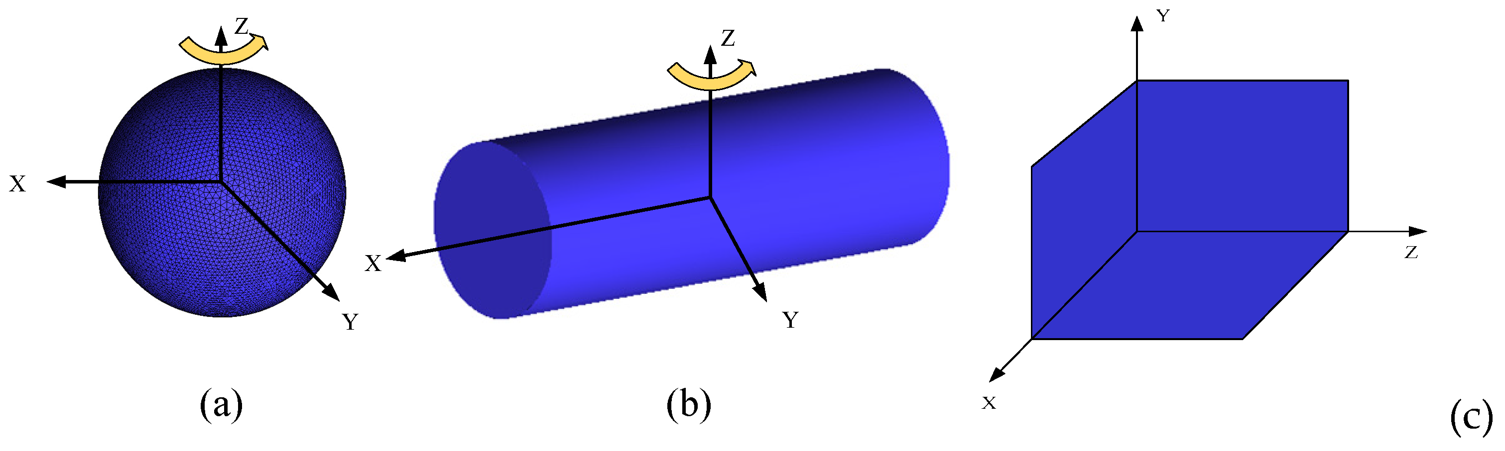
Target	Size (m)	Maximum Mesh Size	Triangle Number	Node Number
Sphere	$2\mathrm{m}\times 2\mathrm{m}\times 2\mathrm{m}$	$0.05\left(0.5\mathsf{\lambda }\right)$	11,000	5628
Cylinder	$2\mathrm{m}\times 2\mathrm{m}\times 6\mathrm{m}$	$0.05\left(0.5\mathsf{\lambda }\right)$	32,328	16,445
Corner reflector	$62\mathrm{m}\times 7.5\mathrm{m}\times 11\mathrm{m}$	$0.1\left(1\mathsf{\lambda }\right)$	294,850	147,427

.

To calculate the TS value of the targets, the incident direction is rotated around the Z axis from 0 degree to 180 degrees with the interval of 1 degree at a frequency of 15 KHz, and $\mathsf{\phi }={90}^{°}$. Moreover, when the frequency is fixed, the ray tube size of the grid on the virtual aperture is smaller and the TS value of the targets is more accurate. For the conventional SBR algorithm, the number of ray tubes at a specified incident direction are listed in

Table 3. The number of ray tubes at a specified incident direction in conventional SBR.

	Sphere	Cylinder	Corner Reflector
Angle	$0.15\mathrm{mm}\left(0.0015\mathsf{\lambda }\right)$	$0.5\mathrm{mm}\left(0.005\mathsf{\lambda }\right)$	$3\mathrm{mm}\left(0.03\mathsf{\lambda }\right)$
0°	13,327 × 13,327	3999 × 3999	3667 × 2500
${60}^{°}$		3999 × 14,469	3667 × 18,431
${90}^{°}$		3999 × 14,399	3667 × 20,500

.

The target strength is defined as

$$\mathrm{TS}=10\lg {\left|\frac{I_r}{I_i}\right|}_{\mathit{r}=1}$$

(5)

with $I_i$ and $I_r$ being the incident intensity and echo intensity of sound waves, and $I_r{|}_{r=1}$ being the echo intensity at 1 m from the equivalent acoustic center of the target. A rigid sphere of radius a that satisfies $\mathrm{ka}\gg 1$ and has a target strength of

$$\mathrm{TS}=10\lg \frac{a^2}{4}$$

(6)

and the theoretical TS value of a rigid sphere with a radius of 1 m is −6 dB. What’s more, for a cylindrical object of length L and radius a, as shown in Figure 6, the target strength is expressed as

$$\mathrm{TS}=10\lg \left[\frac{a{L}^2}{2\lambda }{\left(\frac{\sin \beta }{\beta }\right)}^2{\cos }^2\theta \right]$$

(7)

When the radius, length of cylinder and wavelength are set to 1 m, 6 m and 0.1 m, respectively, the TS value of the ends and abeam direction of the cylinder is 32.69 dB and 22.56 dB.

For the conventional SBR algorithm, we only compare the GPU-based SBR result with its theoretical value. Figure 7 illustrates that the TS value of the underwater target that is calculated by the conventional SBR algorithm shows good agreement with the theoretical value that is introduced above. Moreover, as shown in Figure 7a, the mean square error of the data is 0.05; this deviation may be partly due to the fact that invalid ray tubes do not participate in calculating the field integral field integral, and the ideal situation is that the entire target surface participates in the field integral. Figure 8 demonstrates that the TS value of the target has a good convergence effect at high frequencies.

The corner reflector as illustrated in Figure 9 is the international standard benchmark model. The sonar TS result of the corner reflector at a 15 KHz frequency based on GPU is shown in Figure 9, compared with the result that is calculated by the PEM method. It shows that the trend of the corner reflector TS curve based on the SBR algorithm is consistent with the PEM. Moreover, the TS of the bow and the stern is significantly less than the TS of the hull and is consistent with the corner reflector echo characteristics. As illustrated above, the numerical results verify the accuracy of calculating the TS by the conventional SBR algorithm.

In SBR algorithm, the ray-tracing process considers the multiple reflection of sound waves and improves the spatial and frequency domain information integrity of the underwater targets. Due to the memory limitation on the GPU, we divide the virtual aperture plane equally into several portions of the conventional SBR. Based on the principle of reducing the number of ray tubes and saving running memory, an accelerated multiresolution SBR algorithm based on GPU to predict the TS value is proposed.

The comparison of the results between the GPU-based multiresolution SBR and the GPU-based SBR is shown in Figure 10. It is observed that the results of the GPU-based multiresolution SBR has good agreement with the GPU-based conventional SBR.

4.2. Algorithm Runtime Evaluation

The initial size of the ray tubes of the three targets described in Figure 6 are set to 0.012$\mathsf{\lambda }$ (1.2 mm); 0.04$\mathsf{\lambda }$ (4 mm); and 0.24$\mathsf{\lambda }$ (24 mm), respectively, and the threshold of the number of subdivision is three times.

Table 4. The comparison of average runtime per angle of three targets at 15 KHz.

Targets	CPU-Based SBR	GPU-Based SBR	GPU-Based MSBR	Speedup Ratio (CPU)	Speedup Ratio (GPU)
Sphere	4336.35 s	4.45 s	418.65 ms	974.68	10.65
Cylinder	1390.06 s	1.46 s	389.28 ms	897.97	3.75
Corner reflector	924.41 s	1.20 s	499.44 ms	768.42	2.41

summarizes the average runtime per angle at 15 KHz on the CPU-based SBR, GPU-based SBR and GPU-based multiresolution SBR.

As illustrated in Table 4, GPU-based SBR is more than 750 times faster than CPU because of the super high computing power of GPU. Further, the proposed GPU-based accelerated multi-resolution SBR improves runtime performance by at least 2.4 times that of GPU-based SBR, and the main advantage of GPU-based multi-resolution SBR is the saving of running memory on GPU. Furthermore, in [18], GPU MSBR is about 40 times faster than CPU MSBR, and at least 4.8 times faster than GPU-based SBR without a multi-resolution mesh algorithm. Compared with [18], the algorithm in this paper sees an improvement in the speedup ratio.

5. Discussion

Underwater target strength prediction attaches great importance to many applications. The GPU-accelerated SBR implementation in this article reveals the great potential of accurate target strength prediction. The performance is much improved compared with the traditional panel element method. We will continue to develop more accurate algorithms based on current works.

6. Conclusions

In this paper, we discussed the GPU-accelerated multiresolution SBR algorithm to calculate the target strength of underwater targets. By means of comparing with the theoretical value and the literature, our numerical results showed good agreement. Moreover, compared with the experiment results on the CPU and GPU, the proposed approach achieves 750× speedup and improved the runtime performance efficiently. The next stage of the work will be porting the code to a multi-GPU platform, further realizing the real-time prediction of the target strength of underwater targets.

References

- Odom, R.I. An Introduction to Underwater Acoustics: Principles and Applications. Eos Trans. Am. Geophys. Union 2003, 84, 265. [Google Scholar] [CrossRef][Green Version]
- Fang, Y.Y.; Cheng, K.A.; Sung, P.J.; Chao, C.H.; Chen, C.F. Study of target strength of underwater vehicle. In Proceedings of the Underwater Technology IEEE, Busan, Korea, 21–24 February 2017. [Google Scholar]
- Tang, W. Calculation of acoustic scattering of a nonrigid surface using physical acoustic method. Chin. J. Acoust. 1993, 3, 226–234. [Google Scholar]
- Tang, W. Calculation of acoustic scattering from object near an interface using physical acoustic method. Acta Acust. 1999, 10, 1–5. [Google Scholar]
- Li, W.; Li, J. Underwater acoustic scattering of a Bessel beam by rigid objects with arbitrary shapes using the T-matrix method. In Proceedings of the 2012 Oceans, Hampton Roads, VA, USA, 14–19 October 2012. [Google Scholar]
- Yang, P.; Yuan, B.C.; Zhou, S.; Wen, G. Graphical Acoustics Computing Method for Highlight Characteristics Calculation of Underwater Targets Echoes. J. Syst. Simul. 2009, 21, 3898–3901. [Google Scholar]
- Fan, J.; Tang, W.L.; Zhuo, L.K. Planar elements method for forecasting the echo characteristics from sonar targets. J. Ship Mech. 2012, 16, 171–180. [Google Scholar]
- Chen, W.; Sun, H.; Wang, W. Study on calculation method of target strength in waveguide. In Proceedings of the 2016 IEEE/OES China Ocean Acoustics (COA), Harbin, China, 9–11 January 2016. [Google Scholar]
- Naiwei, S.; Jianchen, L.; Yamin, W. Simulation of Submarine Target Strength Forecast Based on Improved Planar Element Method. Torpedo Technol. 2016, 24, 254–258. [Google Scholar]
- Liu, C.Y.; Zhang, M.M.; Cheng, G.L.; Xu, G.J. Improved planar element method for computing target echo. J. Nav. Univ. Eng. 2008, 20, 25–27. [Google Scholar]
- Ling, H.; Chou, R.C.; Lee, S.W. Shooting and bouncing rays: Calculating the RCS of an arbitrarily shaped cavity. Antennas Propag. IEEE Trans. 1989, 37, 194–205. [Google Scholar] [CrossRef]
- Ling, H.; Chou, R.; Lee, S. Shooting and bouncing rays: Calculating RCS of an arbitrary cavity. In Proceedings of the 1986 Antennas and Propagation Society International Symposium, Philadelphia, PA, USA, 8–13 June 1986. [Google Scholar]
- Tao, Y.; Lin, H.; Bao, H. GPU-Based Shooting and Bouncing Ray Method for Fast RCS Prediction. IEEE Trans. Antennas Propag. 2010, 58, 494–502. [Google Scholar]
- Kee, C.Y.; Wang, C.F. Efficient GPU Implementation of the High-Frequency SBR-PO Method. IEEE Antennas Wirel. Propag. Lett. 2013, 12, 941–944. [Google Scholar] [CrossRef]
- Tao, Y.B.; Lin, H.; Bao, H. KD-Tree Based Fast Ray Tracing for RCS Prediction. Prog. Electromagn. Res. 2008, 81, 329–341. [Google Scholar] [CrossRef]
- Suk, S.; Seo, T.I.; Park, H.S.; Kim, H.T. Multiresolution grid algorithm in the SBR and its application to the RCS calculation. Microw. Opt. Technol. Lett. 2001, 29, 394–397. [Google Scholar] [CrossRef]
- Bang, J.K.; Kim, B.C.; Suk, S.H.; Jin, K.S.; Kim, H.T. Time Consumption Reduction of Ray Tracing for Rcs Prediction using Efficient Grid Division and Space Division Algorithms. J. Electromagn. Waves Appl. 2007, 21, 829–840. [Google Scholar] [CrossRef]
- Gao, P.C.; Tao, Y.B.; Lin, H. Fast RCS Prediction Using Multiresolution Shooting and Bouncing Ray Method on the Gpu. Prog. Electromagn. Res. 2010, 107, 187–202. [Google Scholar] [CrossRef]
- Sengupta, S.; Harris, M.; Zhang, Y.; Owens, J.D. Scan Primitives for GPU Computing. In Proceedings of the Acm Siggraph/eurographics Symposium on Graphics Hardware Eurographics Association, San Diego, CA, USA, 4–5 August 2007. [Google Scholar]