An Automatic Partition Time-Varying Markov Model for Reliability Evaluation

Abstract

As the service time of mechanical devices is getting longer and longer, the safe and reliability evaluation during operation is highlighted. Moreover, real-time reliability evaluation with consideration of multi-state performance degradation becomes increasingly important nowadays, since the consequences of sudden failures are more unacceptable than ever before. The Markov process is a commonly used model in multi-state reliability evaluation. However, little research of the Markov model can deal with multi-source monitoring data and time-varying properties of device performance degradation, as well as the scientific state number determination. In this article, a real-time reliability evaluation model based on automatic partition and the time-varying Markov chain is proposed to solve the problems of the scientific state number selection and time-varying properties description with the state transition matrix of the Markov process, together with taking advantage of multi-source information. The effectiveness of the proposed algorithm is demonstrated on the bearing with life-long vibration and temperature data. It shows that the proposed automatic partition time-varying Markov model can decide the state number automatically according to the trend of life-long data, and evaluate real-time reliability based on equipment operating hours and operating status. The result of predicted remaining useful life obtained by the proposed model is more accurate, and it also shows great superiority in conformity with reality.

1. Introduction

With the continuous improvement of design and manufacturing technology, as well as the materials used, service time of mechanical devices is getting longer and longer, especially in the field of rail transit. For instance, the design service life of bearing on a bogie axle box is more than 20 years. These products usually have only a small number of failures or no failures in life tests, including accelerated life test methods. However, the traditional reliability evaluation methods such as fault tree analysis (FTA) [1], event tree analysis (ETA) [2], and failure mode effects and criticality analysis (FMECA) [3], etc. mainly focus on the “average” characteristics of the same kind of product with fault record data. There is an insurmountable gap of these methods in describing the performance degradation of specific components. Moreover, devices with the same type have different degradation trajectories under different operating environments [4]; even devices of the same type with the same operating environments may also have different degradation trajectories, caused by randomness in the manufacturing process or other unexpected factors. Since real-time reliability evaluation becomes increasingly important nowadays, performance monitoring data is generally used for reliability evaluation of the specific product, instead of traditional failure records. Thanks to the rapid development of sensor technology, more and more data for the service performance evaluation and reliability analysis hasve been provided, which greatly improves the possibility of accurate reliability evaluation and prediction.

The concept of reliability analysis based on performance degradation data was first proposed by Gertsbackh and Kordonskiy in 1969 [5]. Since then, many experts and scholars have started exploratory research in this area. At present, it can be mainly divided into two kinds of performance degradation reliability analysis methods based on regression model and stochastic process. A simple regression model is used in the escalators Avante model based on time series analysis [6]. The effect of variable amplitude service loading conditions and wear phenomenon are investigated based on nonlinear regression reliability analysis for rail steel [7]. Reference [8] combined the fault data with the state detection data of performance degradation, and used the DTS (Degradation Threshold Shock) method to analyze the reliability with competitive failure phenomenon. The commonly used stochastic processes are mainly the Wiener processes [9,10], Gamma process [11], Poisson process [12], Markov process [13], etc. Some reliability analysis methods generally assume that the device only has two states (normal and failure) [14,15,16]. The potential changes during device degradation had been ignored, which made the reliability results too crude to guide practical application. Compared with two-state (normal, fault) reliability analysis models, the multi-state model is more suitable for actual equipment operation. Reference [17] provided a reliability evaluation framework based on multi-performance conversion, which is conducted on the conversion capabilities of the components. A multi-state physics model for dynamic reliability evaluation with the crack propagation state transitions and the Forman model is proposed for a multi-cracked structure [18]. As a powerful tool for multi-state performance degradation modeling, the Markov process of different types has obtained many achievements, such as discrete time Markov process (DTMP) [19,20], continuous time Markov process (CTMP) [21,22], discrete-time hidden aging Markov process (DTHAMP) [23,24], nonhomogeneous continuous-time hidden Markov process (NHCTHMP) [25,26], homogeneous discrete-time hidden semi-Markov process (HDTHSMP) [27,28,29], etc. However, the number of device states was set directly, which may not objectively reflect the overall trend of the device’s performance and may lead to a decrease in model accuracy. Very few pieces of literature have studied the actual number of the device’s states. Reference [30] achieved the optimal number of states by multiple trials under different states number with BIC and AIC as evaluation indicators. However, the time-consuming problem stands out with the increase of available data. Besides that, the state transition matrix of most Markov models is fixed, which means no matter how the device performance degraded, the device reliability does not change when it is detected in a certain state of such a Markov model. In fact, the longer the system or device stays in a certain state, the greater the probability of transitioning out of the state, so these mentioned Markov models cannot reflect the performance degradation within the same state interval over time, which is not in line with reality [31]. That is a great obstacle in dealing with time-varying characteristics of device performance. Moreover, most degradation reliability evaluation methods, especially for mechanical devices, are based on single monitoring data, such as vibration data. Multi-source monitoring is the trend of device performance condition monitoring, and more information is provided for accurate detection and prediction [32]. How to make full use of multi-source data is an urgent problem to be solved.

Hence, in this article, a real-time reliability evaluation model based on the automatic partition method and time-varying Markov chain is proposed, in which the automatic partition is utilized to select the state number of Markov processes scientifically, while the time-varying properties of device performance are described by the time-varying transition matrix of the Markov process. The rest of this article is structured as follows. The basic concept of Tsallis entropy working as data features is presented in Section 2, first. Then the framework of the proposed real-time reliability evaluation algorithm based on automatic partition time-varying Markov process is illustrated. An experiment is carried out in Section 3 to demonstrate the superiority of the proposed algorithm. In particular, it is conducted on bearing with a condition monitoring vibration signal in two directions and a temperature signal. The article is summarized in Section 4.

2. Materials and Methods

2.1. Tsallis Entropy

Tsallis entropy is non-extensive entropy; it is an expression of entropy with exponent q proposed by Brazilian physicist Constantino Tsallis in 1988 [33]. Its mechanism is based on the non-extensive statistics derived from the Boltzmann–Gibbs theory. The Tsallis entropy performs very well in the description of the system with long-range interactions, long-term memory effects, or systems evolving in a multifractal-like space-time. Due to the above characteristics, the Tsallis entropy has a wide range of applications in many fields, such as physics, medicine, and economics. The Tsallis entropy is concave, stable, and is limited in the rate of entropy generation per unit time [34]. Although Shannon entropy, Renyi entropy, etc., have very rich applications in the field of bearing analysis, these entropies are not good enough to describe the bearing performance degradation with vibration signal. Therefore, the Tsallis entropy is extracted as the data featured from the vibration signal in this article. The definition is as below:

$$H_q^T=\frac{1}{q-1}(1-{\displaystyle \sum _{i=1}^n{p}_i^q})$$

(1)

where $q$ describes the non-extension degree of the target object. In this research, it represents the long-range correlation of time series data. $n$ is the total data number in one sample. $p_i$ is the $i$-th value of the sample.

The purpose of Tsallis entropy is to find a clear $q$ value (generally not equal to 1) to describe as much as possible the phenomenon that is neither regular nor completely chaotic or random. After many experiments, we found that $q=2$ can better describe the changing characteristics of bearing.

2.2. The Automatic Partition Time-Varying Markov Model for Reliability Evaluation

The reliability analysis method based on the automatic partition time-varying Markov process mainly includes five steps: degradation feature extraction, state number decision, training data preparation, time-varying Markov process modeling, and reliability assessment. The automatic partition method is used to automatically divide the component degradation sample data into multiple stages, to avoid the artificial and time-consuming selection of the number of Markov process states. In the data processing procedure, in order to deal with the different degradation processes of bearings, the slope-based dynamic time warping method is used to effectively regularize the collected samples, so as to get more accurate bearing Markov model. On the basic Markov process, a time-varying transition probability matrix is proposed to describe the changing trend of the device’s own characteristics with time, which provides a necessary means for more accurate assessment of device state reliability and life prediction. The functions for reliability and remaining useful life are provided at the last step.

The basic steps are provided as follows and shown in Figure 1.

(1) Extract feature on the full-life-running vibration data.

(2) The automatic partition method is used to decide the state number of Markov model, corresponding to the degradation state of device.

(3) Prepare training data. The slope-based dynamic time warping method is used for sample time warping to complete the sample data processing in this step.

(4) Establish the time-varying Markov model. The model parameters are re-estimated using the conditional probability formula for calculating the initial forward probability, backward probability, and state sequence.

(5) Reliability and remaining useful life calculation and prediction. Determine the current state and obtain the sojourn time in the current state, $i$. Then, calculate it in the remaining states $i+1,i+2,\dots ,N$. Calculate the reliability and remaining useful life of the equipment with current state, $i$, and sojourn time, $s{t}_t^i$.

2.2.1. The Automatic Partition Method for State Number Determination of the Markov Model

The automatic partition method based on fuzzy time series segmentation is used to automatically obtain the state number of the Markov model.

It is assumed that $x_l$ is an $M$ dimensional multivariate sample, and $S$ is the sample sequence with length, $L$, where $S=\{d_l={[t_l,x_l^T]}^T|1\le l\le L\}$, $x_l=\left\{x_{lm}|m=1,2,\dots ,M\right\}$. According to the trend of data change, that is based on the equipment performance degradation, sample sequence S can be partition into several segments.

In this article, sample sequence $S$ is assumed to be divided into $P$ segments, noted as $Su{b}_S^P=\left\{Su{b}_S^p|p=1,2,\dots ,P\right\}$, and the boundaries are $s_1<s_2<\cdots s_P$, where $s_1,s_2,\dots ,s_P\in S$ and $s_1=d_1,s_P=d_L$. That is, $Su{b}_S^p=(s_{p-1}+1,s_p),p=1,2,\dots ,P$.

Define the sample sequence segmentation objective function as $C(Su{b}_S^P)$.

$$C(Su{b}_S^P)={\displaystyle \sum _{p=1}^{P}C(Su{b}_S^p)}={\displaystyle \sum _{p=1}^{P}C(s_{p-1}+1,s_p)}$$

(2)

The objective function is generally represented as the distances between the monitoring data in each segment and their corresponding fitting function.

$$C(Su{b}_S^P)={\displaystyle \sum _{p=1}^P{\displaystyle \sum _{l=s_{p-1}+1}^{s_p}{\Vert x_l-v_p^x\Vert }^2}}={\displaystyle \sum _{p=1}^P{\displaystyle \sum _{l=1}^L{\beta }_p(t_l)D^2(x_l,v_p^x)}}$$

(3)

where $v_p^x$ is the cluster center of the $p$-th segment, $D^2(x_l,v_p^x)$ is the distance between $x_l$ and $v_p^x$, ${\beta }_p(t_l)$ is the membership function of $x_l$ subordinate to the $p$-th segment.

The objective function mentioned above is minimized to obtain the segment boundaries with optimal segment positions $s_{p-1}+1,s_p,p=1,2,\dots ,P$. It is generally conducted by various heuristic algorithms.

${\beta }_p(t_l)$ is defined as a (0, 1) binary function in references [35,36], which is not appropriate in practice. In this article, the multivariate mixture Gaussian function is introduced into a cluster prototype as the sequence fitting function to describe the fuzzy characteristic of boundaries between segments. The optimal segment positions are obtained by minimizing the weighted sum of squared distances between the monitoring data in each segment and the center of the cluster prototype.

$$C(Su{b}_S^P)={\displaystyle \sum _{p=1}^P{\displaystyle \sum _{l=1}^L{\left({\mu }_{p,l}\right)}^m{D}^2(d_{{}_l},{\eta }_p)}}$$

(4)

where ${\mu }_{p,l}$ is the membership of $d_l={[t_l,x_l^T]}^T$ belonging to the $p$-th segment, $p=1,2,\dots ,P$; $m=[1,\infty )$ is the weighted index of fuzzy clustering, generally taking $m=2$ [37]; $D^2(d_{{}_l},{\eta }_p)$ represents the distance between the monitoring data in each segment and the center of the cluster prototype; ${\eta }_p$ is the clustering prototype function of $p$-th segment.

It is assumed that the expectation and the covariance matrix of the used multivariate Gaussian distribution for sample sequence are $v_p$ and $F_p$, respectively. The probability density function $f({\mathit{d}}_l|\eta )$ denoting the adscription of monitoring data to the $p$-th segment is

$$f({\mathit{d}}_l|\eta )={\displaystyle \sum _{p=1}^{P}f({\mathit{d}}_l{|\eta }_p)f({\eta }_p)}$$

(5)

where $f(\mathit{d}{|\eta }_p)=\frac{1}{{(2\pi )}^{(n+1)/2}\sqrt{\det (F_p)}}\exp (-\frac{1}{2}{(d-{\mathrm{v}}_p)}^T{(F_p)}^{-1}(d-{\mathrm{v}}_p))$; $f({\eta }_p)$ is the unconditional clustering probability, ${\displaystyle \sum _{p=1}^{P}f({\eta }_p)=1}$; ${\eta }_p$ is the clustering prototype function of the $p$-th segment, ${\eta }_p=\{f({\eta }_p),{\mathrm{v}}_p,F_p|p=1,2,\dots ,P\}$.

According to probability theory, the distance function and the membership in the $p$-th segment are inversely proportional based on the Gath–Geva clustering algorithm [38]. The time and feature variables of sample sequence are independent with each other. Then,

$$\begin{array}{ll}f({\mathit{d}}_l{|\eta }_p)& =\frac{1}{D^2({\mathit{d}}_l,{\eta }_p)}\\ & =\underset{p({\eta }_p)}{\underbrace{{\alpha }_p}}\underset{p(t_l|{\eta }_p)}{\underbrace{\frac{1}{\sqrt{2\pi {\sigma }_{p,t}^2}}\exp (-\frac{1}{2}\frac{{(t_l-v_p^t)}^2}{{\sigma }_{p,t}^2})}}\times \underset{p({\mathrm{x}}_l|{\eta }_p)}{\underbrace{\frac{1}{{(2\pi )}^{r/2}\sqrt{\det (A_p)}}\exp (-\frac{1}{2}{({\mathrm{x}}_l-{\mathrm{v}}_p^x)}^T{(A_p)}^{-1}({\mathrm{x}}_l-{\mathrm{v}}_p^x))}}\end{array}$$

(6)

where ${\alpha }_k$ is the initial probability of clustering, $\frac{1}{\sqrt{2\pi {\sigma }_{p,t}^2}}\exp (-\frac{1}{2}\frac{{(t_l-v_p^t)}^2}{{\sigma }_{p,t}^2})$ is the distance between the time variable and the clustering center of time variable, $\frac{1}{{(2\pi )}^{r/2}\sqrt{\det (A_p)}}\exp (-\frac{1}{2}{({\mathrm{x}}_l-{\mathrm{v}}_p^x)}^T{(A_p)}^{-1}({\mathrm{x}}_l-{\mathrm{v}}_p^x))$ is the distance between the feature variable in the $l$-th sample and the feature cluster center, $v_p^x$ is the feature cluster center of $p$-th segment, and $r$ is the rank of the feature variable distance norm, $A_p$.

There are many ways to calculate the distance norm $A_p$. Mahalanobis distance is a good choice and can be used to adjust the correlation between variables. Let $A_p=F_p$, where $F_p$ is the fuzzy covariance matrix of the multivariate Gaussian distribution,

$$F_p=\frac{{\displaystyle \sum _{l=1}^L{({\mu }_{p,l})}^m{(({\mathrm{x}}_l-{\mathrm{v}}_p^x){({\mathrm{x}}_l-{\mathrm{v}}_p^x)}^T)}^T}}{{\displaystyle \sum _{l=1}^L{({\mu }_{p,l})}^m}}$$

(7)

Principal Component Analysis (PCA) is introduced to eliminate the strong correlations between variables while reducing dimensionality.

It is assumed that ${\lambda }_{p,q},q=1,2,\dots ,Q$ are the $Q$ non-zero eigenvalues of $F_p$ in descending order. Their corresponding eigenvectors are $u_{p,q},q=1,2,\dots ,Q$. It can be obtained that:

$$F_p=U_p{\Lambda }_p{U}_p^T$$

(8)

$${\Lambda }_p=\left|\begin{array}{cccc}{\lambda }_{p,1}& & & \\ & {\lambda }_{p,2}& & \\ & & \ddots & \\ & & & {\lambda }_{p,Q}\end{array}\right|$$

(9)

$$U_p=[u_{p,1},u_{p,2},\dots ,u_{p,Q}]$$

(10)

The feature variables of the sample sequence are reduced to Q-dimension by the PCA method, and $y_{p,l}=W_p^{-1}({\mathrm{x}}_l)=W_p^T({\mathrm{x}}_l)$ is obtained, where $W_p=U_{p,Q}{\Lambda }_{p,Q}^{1/2}$.

According to probabilistic principal component analysis [39], $W_p=U_{p,Q}{({\Lambda }_{p,Q}^{}-{\sigma }_{p,x}^{2}I)}^{1/2}{R}_{pS}$, where $R_p$ is a $Q\times Q$ orthogonal transformation matrix, ${\sigma }_{p,x}^2=\frac{1}{M-Q}{\displaystyle \sum _{j=Q+1}^M{\lambda }_{p,q}}$.

Until now, the automatic partitioning algorithm of fuzzy segmentation has been transformed into an operational research optimization problem. The model is shown below,

$$C(Su{b}_S^P)={\displaystyle \sum _{p=1}^P{\displaystyle \sum _{l=1}^L{\left({\mu }_{p,l}\right)}^m{D}^2(d_{{}_l},{\eta }_p)}}$$

(11)

$$\begin{array}{ll}U={[{\mu }_{p,l}]}_{P\times L},& {\mu }_{p,l}\in [0,1],\forall p,l\\ {\displaystyle \sum _{p=1}^P{\mu }_{p,l}=1,}& \forall l\\ 0<{\displaystyle \sum _{l=1}^L{\mu }_{p,l}}<L,& \forall p\end{array}$$

(12)

The alternate optimization algorithm and the Picard iterative algorithm can be used to solve this problem.

The basic steps are as follows:

(1)

Initialization

The initial segments number of $S$ and the dimension of the eigenvector space are given at first. Then, select the appropriate stopping condition, $\epsilon ,\epsilon >0$, and initialize $W_p,{\mathrm{v}}_p^x,{\sigma }_{p,x}^2,{\mu }_{p,l}$;

(2)

Loop calculation.

(i)

Calculate the cluster prototype ${\eta }_p$.

Cluster initial probability:

$${\alpha }_p=\frac{1}{L}{\displaystyle \sum _{l=1}^L{\mu }_{p,l}}$$

(13)

Cluster center:

$${\mathrm{v}}_p^x=\frac{{\displaystyle \sum _{l=1}^L{({\mu }_{p,l})}^m({\mathrm{x}}_l-W_p\langle y_{p,l}\rangle )}}{{\displaystyle \sum _{l=1}^L{({\mu }_{p,l})}^m}}$$

(14)

where $\langle y_{p,l}\rangle =M_p^{-1}{W}_p^T(x_l-v_p^x)$, $M_p={\sigma }_{p,x}^{2}I+W_p^T{W}_p$;

Weight update:

$${\tilde{W}}_p=F_p{W}_p{({\sigma }_{p,x}^{2}I+M_p^{-1}{W}_p^T{F}_p{W}_p)}^{-1}$$

(15)

Variance update:

$${\sigma }_{p,x}^2=\frac{1}{Q}tr(F_p-F_p{W}_p{M}_p^{-1}{\tilde{W}}_p^T)$$

(16)

Distance norm:

$$A_p={\sigma }_{p,x}^{2}I+{\tilde{W}}_p{\tilde{W}}_p^T$$

(17)

Calculation of cluster prototype center and standard deviation parameter of time parameter for sample sequence:

$$v_p^t=\frac{{\displaystyle \sum _{l=1}^L{({\mu }_{p,l})}^m{t}_l}}{{\displaystyle \sum _{l=1}^L{({\mu }_{p,l})}^m}},{\sigma }_{p,t}^2=\frac{{\displaystyle \sum _{l=1}^L{({\mu }_{p,l})}^m{(t_l-v_p^t)}^2}}{{\displaystyle \sum _{l=1}^L{({\mu }_{p,l})}^m}}$$

(18)

(ii)

Cluster merging

The similarity factor, $S_{PCA}^{a,b}$, based on PCA proposed by Krzanowski is applied as one of the merging criteria for two adjacent segments, $Su{b}_S^a,Su{b}_S^b$, to determine whether they need to be merged or not.

$$S_{PCA}^{a,b}=\frac{1}{Q}{\displaystyle \sum _{a=1}^Q{\displaystyle \sum _{b=1}^Q{\cos }^2{\theta }_{a,b}}}=\frac{1}{Q}tr(U_{a.q}^T{U}_{b,Q}{U}_{b.Q}^T{U}_{a,Q})$$

(19)

where $U_{a,Q},U_{b,Q}$ are the first $Q$ eigenvalues of the eigenvectors for segments $Su{b}_S^a$ and $Su{b}_S^b$, respectively.

The distance between the cluster centers of $Su{b}_S^a$ and $Su{b}_S^b$ is another merging criterion.

$$D(v_o^x,v_p^x)=\Vert v_o^x-v_p^x\Vert$$

(20)

Since the clustering process is carried out in the whole range of $S$, the clustering similarity of each state space is measured by the fuzzy decision algorithm proposed by $U$. Kaymak et al. are featured in [40], in which the overall similarity matrix is $H=\left\{h_{a,b}|1\le a\le P,1\le b\le P\right\}$,

$$h_{a,b}=\sqrt{\frac{{\left(\frac{1}{P(P-1)}{\displaystyle \sum _{a=1}^P{\displaystyle \sum _{\begin{array}{l}b=1\\ b\ne o\end{array}}^P{S}_{PCA}^{a,b}}}\right)}^2+{\left(\frac{1}{P(P-1)}{\displaystyle \sum _{a=1}^P{\displaystyle \sum _{\begin{array}{l}b=1\\ b\ne o\end{array}}^{P}D(v_a^d,v_b^d)}}\right)}^2}{2}}$$

(21)

If the clustering similarity factor, $h_{a,a+1}$, of two adjacent segments, $Su{b}_{{}_S}^a,Su{b}_S^{a+1}$, is exceeded the set threshold, $Su{b}_{{}_S}^a,Su{b}_S^{a+1}$ will be merged. It ends when the algorithm termination condition, $\epsilon$, is reached.

2.2.2. The Time-Varying Markov Model

The automatic segmentation method provides a scientific basis for the states number selection of the Markov process. Moreover, we argue that the transition probability between states is not only related to the state that the device stays, but also related to the sojourn time that the equipment stays in the present state. In practical situations, the longer a device stays in a state, the greater the probability of its transition from that state to another states. That is to say, the state sojourn time affects the state transition probability to a certain extent. Therefore, the state transition matrix (Sojourn time-based state transition probabilities) related to the state sojourn time is introduced to establish a time-varying Markov process for real-time reliability evaluation. The proposed Markov process is noted as $M=(\pi ,A,ST)$, where, $\pi$ is the initial state probability distribution $\pi =\left\{{\pi }_i\right\},1\le i\le N$ and ${\pi }_i=P[s_1=i],1\le i\le N$; $N$ is the state number, which is determined by the automatic partition method mentioned above; $A$ is the time-varying state transition matrix, $A=\{a_{ij}(s{t}_t^i)\},1\le i,j\le N,1\le s{t}_t^i\le S{T}^i$, and $a_{ij}(s{t}_t^i)$ represents the state transition probability of the device transitioning from state $i$ to state $j$ when the device stays in state $i$ at time $t$, ${\displaystyle \sum _{j=1}^N{a}_{ij}(s{t}_t^i)=1},1\le s{t}_t^i\le S{T}^i,1\le i,j\le N$. $S{T}^i$ is the maximum sojourn time in state $i$, and $ST$ is the state sojourn time distribution, which is assumed to obey a Gaussian distribution.

Firstly, according to the sample set, the sojourn time distribution of each state is determined, and then the model parameters are estimated by the improved Baum–Welch algorithm.

(1) When the model parameters $M=(\pi ,A,ST)$ are known, the probability that the device stays in state $i$ for a sojourn time, $T^{*}$, at time $t$ is ${\alpha }_t(i,T_t{}^{i*})=P(q_t=i,s{t}_t^i=T_t{}^{i*}|M)$,

When $t=1$, the initial forward probability is

$${\alpha }_1(1,s{t}_1^i)=1$$

(22)

$${\alpha }_1(j,1)={\alpha }_1(1,s{t}_1^i)a_{1j}(s{t}_1^i)$$

(23)

$${\alpha }_1(N,s{t}_1^N)={\displaystyle \sum _{i=2}^N{\alpha }_1(i,s{t}_1^i=1)P(s{t}_1^i=1)a_{iN}(s{t}_1^i=1)}$$

(24)

When $t=2,3,\dots ,T$, the forward probability recursion formula is

$${\alpha }_t(j,1)={\displaystyle \sum _{\begin{array}{l}i=2\\ i\ne j\end{array}}^{N-1}{\displaystyle \sum _{s{t}_t^i=1}^{S{T}^i}{\alpha }_{t-1}(i,s{t}_t^i)P(s{t}_t^i)a_{ij}(s{t}_t^i)}}$$

(25)

$${\alpha }_t(j,d)={\alpha }_{t-1}(j,s{t}_t^i-1)$$

(26)

$${\alpha }_t(N,s{t}_t^N)={\displaystyle \sum _{i=2}^{N-1}{\displaystyle \sum _{s{t}_t^i=1}^{S{T}^i}{\alpha }_t(i,s{t}_t^i)P(s{t}_t^i)a_{iN}(s{t}_t^i)}}$$

(27)

(2) At time $t$, when the equipment stays in state $i$ for a sojourn time $s{t}_t^i$, the backward probability of producing the state sequence in time $T-t$ is ${\beta }_t(i,s{t}_t^i)=P(s_t=i,s{t}_t^i|M)$.

When $t=T$, the initial backward probability formula is

$${\beta }_T(N,s{t}_T^N)=1$$

(28)

$${\beta }_T(i,s{t}_t^i)=P(s{t}_t^i)a_{iN}(s{t}_t^i)$$

(29)

$${\beta }_T(1,s{t}_1^i)={\displaystyle \sum _{j=2}^{N-1}{\alpha }_{1j}(s{t}_1^i)}{\beta }_T(j,s{t}_1^i)$$

(30)

When $0<t<T$, the backward probability recursion formula is

$${\beta }_t(i,s{t}_t^i)=P(s{t}_t^i){\displaystyle \sum _{\begin{array}{l}j=2\\ j\ne i\end{array}}^{N-1}{\alpha }_{ij}(s{t}_t^i)}{\beta }_{t+1}(j,1)+{\beta }_{t+1}(i,s{t}_t^i+1),1<i<N$$

(31)

$${\beta }_t(1,s{t}_1^i)={\displaystyle \sum _{j=2}^{N-1}{a}_{1j}(s{t}_1^i)}{\beta }_t(j,1)$$

(32)

Based on the forward probability formula and the backward probability formula, the conditional probability formula $S=(s_1,s_2,\dots ,s_T)$, $s_1,s_2,\dots ,s_T\in \{i, 1\le i\le N\}$ of the state vector can be obtained as

$$P_S=P(S|M)={\displaystyle \sum _{i=1}^N{\displaystyle \sum _{s{t}_t^i}^{T_t{}^{i*}}{\alpha }_t(i,s{t}_t^i)}}{\beta }_t(i,s{t}_t^i)$$

(33)

(3) The re-estimated parameters of the time-varying Markov model can be obtained by the formula

$$\begin{array}{l}{\zeta }_t(i,j,st)=p(s_t=i,s_{t’}=j,s{t}_t^i=st|S,M)\\ =\{\begin{array}{ll}\frac{1}{P_S}{\alpha }_t(1,s{t}_t^1)a_{1j}(s{t}_t^1){\beta }_t(j,1),& \hspace{1em}i=1\\ \frac{1}{P_S}{\alpha }_t(1,st)p(s{t}_t^i)a_{ij}(s{t}_t^i){\beta }_{t+1}(j,1),& \hspace{1em}2\le i,j<N\\ \frac{1}{P_S}{\alpha }_t(i,st)p(st)a_{iN}(st){\beta }_{t+1}(j,st),& \hspace{1em}2\le i<N,j=N\end{array}\end{array}$$

(34)

${\zeta }_t(i,j,st)$ is the probability with a given model, $M$, and state sequence of $S=(s_1,s_2,\dots ,s_T)$ and $s_1,s_2,\dots ,s_T\in \{i, 1\le i\le N\}$ show that the performance state of equipment will transit to state $j$, after a sojourn time $st$ in state $i$.

${\gamma }_t(i,st)$ is the probability that when the device stays in state $i$ for a sojourn time, $st$, at time $t$, with a given model of $M$ and state sequence of $S$, ${\gamma }_t(i,st)=p(s_t=i,s{t}_t^i=st|S,M)=\frac{1}{P_S}{\alpha }_t(i,st){\beta }_t(i,st)$.

${\eta }_t(i,st)$ is the probability when the device stays in state $i$ for a sojourn time of $st$ at time of $t$,

$${\eta }_t(i,st)=\frac{1}{P_S}{\alpha }_t(i,st)p(s{t}_t^i=st)[{\displaystyle \sum _{\begin{array}{l}j=2\\ j\ne i\end{array}}^{N-1}{a}_{ij}(st)}{\beta }_{t+1}(j,1)+a_{iN}(st){\beta }_t(N,s{t}_t^N)]$$

(35)

It can be seen from $a_{ij}(st)=p(s_{t+1}=j|s_t=i,s{t}_t^i=st)$ that the revaluation formula of $a_{ij}(st)$ is

$${\overline{a}}_{ij}(st)=\frac{{\displaystyle \sum _{t=1}^T{\zeta }_t(i,j,st)}}{{\displaystyle \sum _{t=1}^T{\eta }_t(i,st)}}$$

(36)

where ${\displaystyle \sum _{t=1}^T{\zeta }_t(i,j,st)}$ is noted as the expected transition number from state $i$ to state $j$, when it stays in state $i$ for a sojourn time, st. ${\displaystyle \sum _{t=1}^T{\eta }_t(i,st)}$ is the sum of expected transition number out of state $i$, when it stays in state $i$ for a sojourn time, st.

Assume that the state sojourn time probability obeys a Gaussian distribution $({\mu }_i,{\sigma }_i^2)$,

$${\overline{\mu }}_i=\frac{{\displaystyle \sum _{t=1}^T{\displaystyle \sum _{st=1}^{T^{i*}}{\eta }_t(i,st)}}\cdot st}{{\displaystyle \sum _{t=1}^T{\displaystyle \sum _{st=1}^{T^{i*}}{\eta }_t(i,st)}}}$$

(37)

$${\overline{\sigma }}_i^2=\frac{{\displaystyle \sum _{t=1}^T{\displaystyle \sum _{st=1}^{T^{i*}}{\eta }_t(i,st)}}\cdot s{t}^2}{{\displaystyle \sum _{t=1}^T{\displaystyle \sum _{st=1}^{T^{i*}}{\eta }_t(i,st)}}}-{\overline{\mu }}_i{}^2$$

(38)

(4) Reliability and remaining useful life prediction

The device in the completely failed segment means that it cannot complete the specified task as required. Therefore, it can be considered that the probability ${\zeta }_t(i,N,st)$ of the device transferring to the completely failed segment, $N$, at time, $t$, with a sojourn time, $st$, is its unreliability. The sum probabilities for device from the current state transferring to every other states is its reliability.

The reliability of a device at different times can be defined as

$$R(t)=1-{\zeta }_t(i,N,st)$$

(39)

The failure rate function is noted as $\lambda (t)$, and its life distribution function is as $F(t)$; density function is $f(t)$,$f(t)=F^{\prime }(t)$, the reliability function is $R(t)$, $F(t)+R(t)=1$, and $\lambda (t)=f(t)/R(t)$. For $\forall t$, there is $R(t)>0$. Therefore, it can be considered that $\lambda (t)$ is an estimate of the interval fault conditional probability.

Let $L$ denote the life cycle of the device and $RUL(t)$ denote the remaining life expectancy of the equipment running normally at time, t, from time, t, to the failure time; there is $RUL(t)=E(L-t|L>t)=(1/R(t)){\displaystyle \underset{t}{\overset{\infty }{\int }}R(x)dx}$.

At time $t^{\ast }$, if the device stays in state $i$ with a sojourn time of $st$, its remaining useful life is equal to the sum of the effective remaining sojourn time of running state $i$ and the remaining time in other remaining states (assuming that it traverses $i+1,i+2,\dots ,N-1$ states).

Among them, the effective remaining sojourn time in operating state $i$ is

$$ru{l}_{t*+st}^i=ru{l}^i\cdot (1-\lambda (t*+st)\cdot \Delta t)=ru{l}^i\cdot (1-\frac{{\zeta }_{t*+st}(i,j,st)}{{\eta }_{t*+st}(i,st)})$$

(40)

where $ru{l}_{t*+st}^i$ is the effective remaining sojourn time when the device stays in state $i$ with a sojourn time of $st$ at time $t^{\ast }$; $ru{l}^i$ is the expected sojourn time in state $i$, $ru{l}^i={\mu }_i$.

Therefore, the remaining useful life for device at time $t^{\ast }$, when it stays in state $i$ with a sojourn time of $st$ can be obtained,

$$RU{L}_{t*+st}^{i,st}=ru{l}_{t*+st}^i+{\displaystyle \sum _{j=i+1}^{N-1}{\mu }_j}$$

(41)

3. Results

Rolling bearing is one of the most widely used general mechanical components in rail vehicles [35]. Only 10~20% of bearings can reach their design life time, according to statistics. They usually cannot work properly due to fatigue, wear, strain, electrical corrosion, fracture, and gluing, etc. Therefore, the bearing is taken as an example to verify the science of the proposed method in this article.

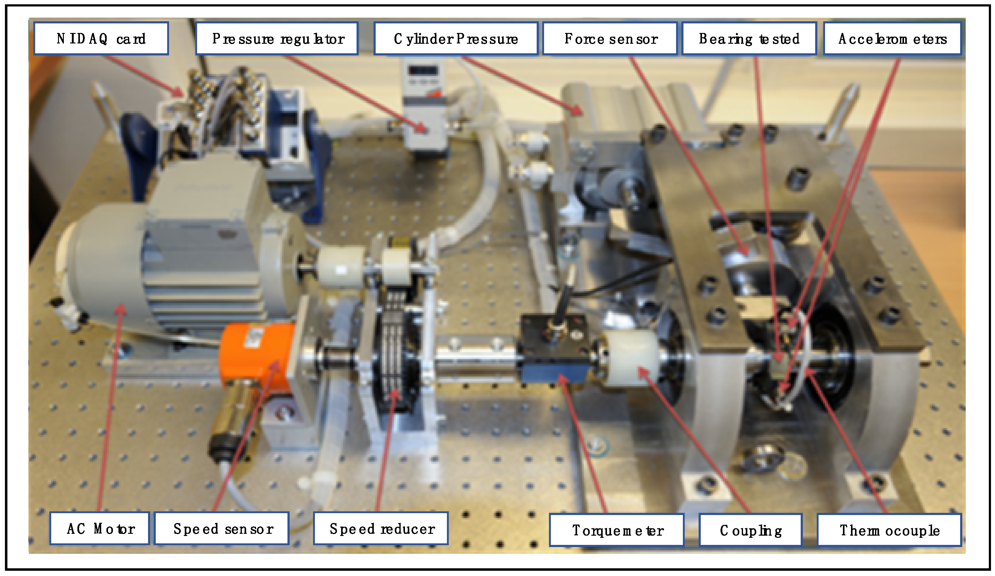
3.1. Experiment Description

The full life data of bearings collected on the PRONOSTIA experimental platform (Figure 2), specially designed and implemented by the AS2M department of the French FEMTO-ST Institute, are used. The PRONOSTIA experimental platform consists of three main parts: the rotating part, the loading part (where radial force is applied on the test bearing), and the measuring part.

The operating conditions of the bearing are measured by the radial force exerted on the bearing, the rotational speed of the bearing, and the torque on the bearing, with a sampling frequency of 100 Hz. The amount of degradation of the bearing is measured by vibration and temperature sensors, and the vibration signal is measured by two placements at a 90-degree angle on the horizontal and vertical axes. The sampling frequency is 25.6 kHz, sampling every 10 s, and each sampling duration of 0.1 s, including 2560 sample points. The temperature sensor is located in the hole near the outer ring of the bearing, with a sampling frequency of 10 Hz and 600 points per minute.

The test dataset used for training in this article is shown in

Table 1. Dataset.

Dataset	Operating Conditions
	Condition 1	Condition 2	Condition 3
Learning set	Bearing1_1	Bearing2_1	Bearing3_1
	Bearing1_2	Bearing2_4
	Bearing1_4
	Bearing1_5
Test set	Bearing1_6	Bearing2_5	Bearing3_3
	Bearing1_7

.

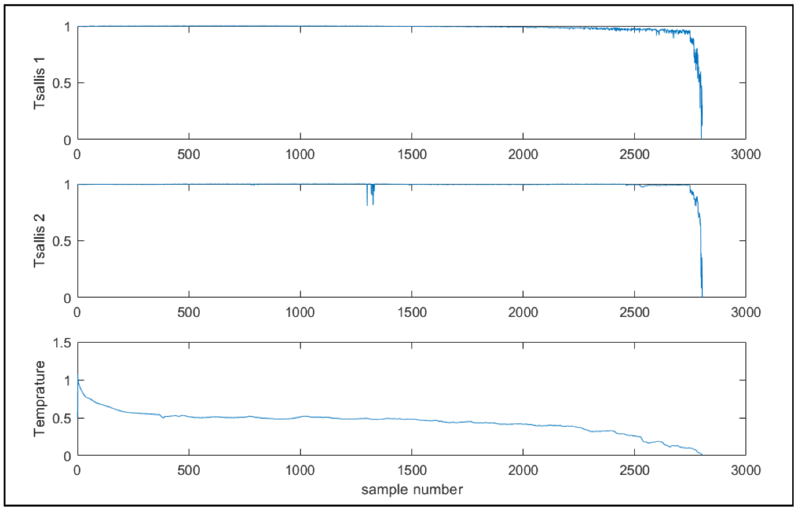
3.2. Feature Extraction

Calculate the entropy of the bearing vibration acceleration data and align the temperature data with the vibration acceleration data. The Tsallis entropy with $q=2$, kurtosis, Shannon entropy, and Renyi entropy were extracted from the same full-life of the bearing vibration signal.

As shown in Figure 3, it can be seen that Shannon entropy and Renyi entropy are not monotonic, and they also fluctuate greatly during the full-life signal period. The trend of the kurtosis value is not obvious enough, and there are some values larger than the failure value, where the sample number ranges from 450 to 900. Those cannot accurately express the performance of the bearing degradation. The Tsallis entropy exhibits monotonic characteristics during the whole life cycle, but also begins to degrade when the bearing performance is not very well (sample number = 1500 in Figure 3) and the numerical stability of the Tsallis entropy is good with bearing degradation.

The bearing temperature signal is resampled to make its length the same as the vibration signal; the maximum value is extracted, and the three groups of signals are normalized respectively to transform it into a dimensionless expression. Taking Bearing1_1 as an example, its characteristic expression is shown in Figure 4.

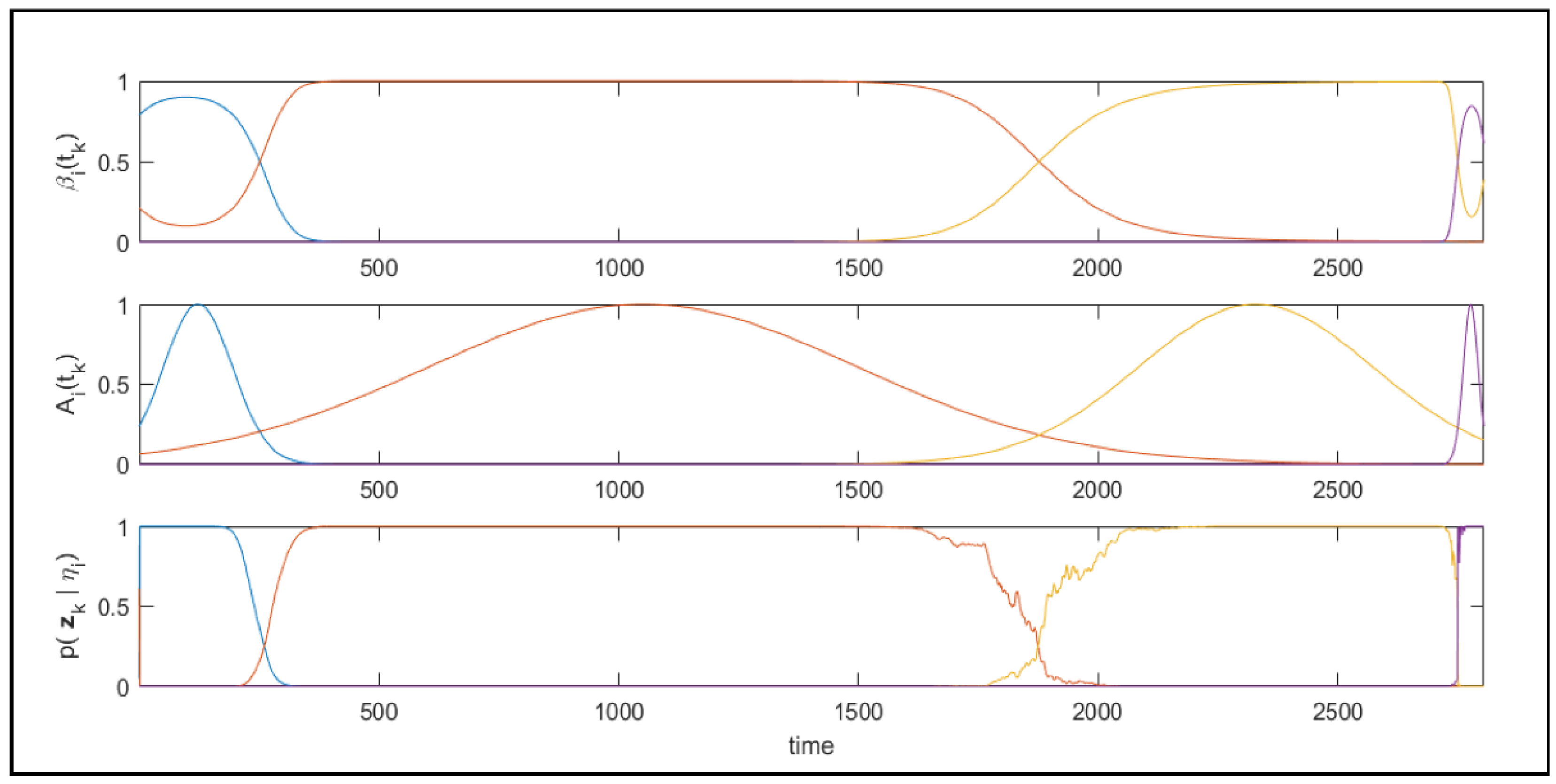
3.3. The Automatic State Number Determination of the Markov Model

The automatic partition method is performed on the feature data of condition 1-bearing 1 in the dataset. The input feature is [Tsallis 1, Tsallis 2, Temperature], and the result is shown in Figure 5.

Therefore, the segmentation results of Bearing1_1 are [0, 360], [361, 1800], [1801, 2740], and [2741, 2803]. That is, the degradation process of the bearing can be divided into four stages, which can be considered as the running-in stage, the normal operation stage, the degradation failure stage, and the complete failure stage. It is consistent with the actual use, which fully verifies the validity and scientific rationality of the multivariate automatic partition algorithm.

The complete failure stage is regarded as the complete failure state; the running-in stage, the normal operation stage, and the degenerate failure stage are denoted as the state 1, the state 2, and the state 3 in this article.

Different bearings have different degradation trajectories. Samples are aligned based on the slope-based dynamic time warping (DTW) method to obtain more accurate training data, according to the change trend of the degradation amount, not the degradation amount. Taking the alignment process of Bearing1_1 and Bearing1_2 as an example, the optimal path for slope alignment, the slope alignment result and sample alignment results are shown in Figure 6, Figure 7 and Figure 8, respectively.

The degradation trends of Bearing1_1 and Bearing1_2 are basically the same, as shown in Figure 8. Based on the segment location of Bearing1_1, the segment location of Bearing1_2 is ([1, 289], [290, 392], [393, 844], and [845, 871]).

However, not every bearing will go through these four degradation stages. In the tested samples, as shown in Figure 9, the Bearing2_4 fails directly without obvious degradation stage. The break-in stage of Bearing2_4 is [1, 402], the degradation failure stage is [403, 740], and the complete failure stage is [741, 751]. It can be concluded that the slope-based dynamic time warping method performed very well for samples that do not fully conform to the degenerate process. It avoids the negative impact caused by confusion of different degradation stages during Markov model training. The segmentation result of dataset is listed in

Table 2. Segmentations result of dataset.

Bearing Number	State 1 Running-in Stage	State 2 Normal Operation Stage	State 3 Degradation Stage	State 4 Complete Failure Stage
Bearing1_1	[1, 360]	[361, 1800]	[1801, 2740]	[2741, 2803]
Bearing1_2	[1, 289]	[290, 392]	[393, 844]	[845, 871]
Bearing1_4	[1, 329]	[330, 1084]	[1085, 1376]	[1377, 1428]
Bearing1_5	[1, 612]	[613, 1020]	[1021, 2421]	[2422, 2463]
Bearing1_7	[1, 540]	[541, 1980]	[1981, 2210]	[2211, 2259]
Bearing2_1	[1, 660]	[661, 817]	[818, 874]	[875, 977]
Bearing2_4	[1, 402]	-	[403, 740]	[741, 751]
Bearing2_5	[1, 566]	[567, 2254]	-	[2255, 2311]
Bearing3_1	[1, 246]	[247, 490]	-	[491, 517]
Bearing3_3	[1, 134]	[135, 294]	[295, 423]	[424, 436]

.

3.4. Reliability Evaluation

In order to verify the validity and accuracy of the state division of mechanical devices of rail transit trains proposed in this article, Bearing1_1, Bearing1_2, Bearing2_1, Bearing2_4, and Bearing3_1 datasets are used for training, and other bearing data are used for testing.

In the time-varying Markov process model, it is assumed that the state transition probability obeys the probability density function of mixed Gaussian distribution, and the probability distribution function of state sojourn time obeys the probability density function of a single Gaussian distribution. Based on the automatic partition method, the state number of the time-varying Markov model is 4, that is $N=4$.

The maximum number of iteration steps is set to be 1000, and the stop criteria of the error convergence is $1\times {10}^{-5}$. The initial matrix of mutual conversion between each state is shown in

Table 3. Initial transformation matrix.

States	State 1	State 2	State 3	State 4
State 1	0.8712	0.1112	0.0173	0.0003
State 2	0.0000	0.7496	0.2511	0.0993
State 3	0.0000	0.0000	0.7028	0.2972
State 4	0.0000	0.0000	0.0000	1.0000

. The average sojourn time in each state can be obtained based on training datasets; its result is shown in

Table 4. Average sojourn time in each state.

States	State 1	State 2	State 3	State 4
Average sojourn time	413.8	739.5	383.9	44.3

. A 4-state, time-varying Markov process reliability and life prediction model is obtained.

The trained time-varying Markov model is updated when a new monitoring data sample is arrived. The bearing staying in state 1 for 10 h is taken as an example. After feature extraction of the monitoring data sample, the data is sent into the trained time-varying Markov model, and state transition matrix is updated at this time. At this time, the state transition matrix is shown in

Table 5. State transformation matrix when bearing stays in state 1 for 10 h.

States	State 1	State 2	State 3	State 4
State 1	0.8695	0.1128	0.0174	0.0003
State 2	0.0000	0.7496	0.2511	0.0993
State 3	0.0000	0.0000	0.7028	0.2972
State 4	0.0000	0.0000	0.0000	1.0000

, while the mean and variance of the state sojourn time are shown in

Table 6. The mathematical expectation and variance of sojourn time when bearing stays in state 1 for 10 h.

States	State 1	State 2	State 3	State 4
Expectation of sojourn time	390.8451	739.5547	383.93594	44.3543
Variance of sojourn time	2.9458	1.5942	1.5026	1.4358

.

The bearing reliability at current time is $R(i=1,s{t}_1=10)=1-0.0003=0.9997$.

To demonstrate the adaptability of the proposed model to changes in time, we also show the model changing parameters when the bearing stays in state 2 for 40 h. At this time, the state transition matrix is shown in

Table 7. State transformation matrix when bearing stays in state 2 for 40 h.

State Number	1	2	3	4
1	-	-	-	-
2	0.0000	0.6512	0.3291	0.1179
3	0.0000	0.0000	0.7028	0.2972
4	0.0000	0.0000	0.0000	1.0000

, while the mean and variance of the state sojourn time are shown in

Table 8. The mathematical expectation and variance of sojourn time when device stays in state 2 for 40 h.

States	State 1	State 2	State 3	State 4
Expectation of sojourn time	-	665.9154	383.9326	44.3427
Variance of sojourn time	-	1.9425	1.5026	1.4358

.

The bearing reliability at current time is $R(i=2,s{t}_1=40)=1-0.1179=0.8821$.

For the bearing used in this experiment, its effective life is the sum of sojourn time in state 1, 2, and 3. When the bearing reaches state 4, it has completely failed. Compared with the hidden Markov model (HMM) algorithm, the prediction result of Bearing1_1 is shown in Figure 10. The lifetime prediction of the HMM presents an obvious step-descent characteristic. Owing to the stable state transition matrix of HMM, the remaining useful life would not change when device performance is detected into a certain state. This characteristic makes the HMM seriously inconsistent with the actual situation.

In contrast, the predicted lifetime of the proposed algorithm in this paper has higher accuracy than HMM, which is in line with the gradual decline with time, since the state transition probability matrix has been designed to update over time theoretically. In addition, the proposed algorithm becomes more and more accurate as the bearing performance gradually degrades; that is, the results of predicted life are more accurate in the later stage. It should be emphasized that there is also a slight step-descent as the red line shown in Figure 10. Because the state transition probability matrix is not changing over time in practice, it is only updated when a new monitoring data sample has arrived. The shorter the interval of condition monitoring data, the smoother the prediction curve would be.

4. Conclusions

The proposed automatic partition time-varying Markov model has two main contributions on real time reliability evaluation, based on the Markov process. Firstly, the state number of Markov processes is selected scientifically on the basis of the device’s performance degradation stages. This work is realized automatically, based on the characteristics of the degradation curve, with full use of the multi-source monitoring data. It is done without manual intervention, and the state number is obtained by taking full advantage of multidimensional information, instead of by only a single threshold. This work builds a good foundation for a time-varying Markov model. The other main contribution is the time-varying Markov model. It describes the timely changing degradation process of device performance. The polymorphic real-time reliability assessment and remaining useful life prediction are achieved in this procedure. From the experiment, the proposed algorithm demonstrates a strong capability for data changes and great potential in accurately performing degradation prediction. This model would be more accurate if the monitoring data points are provided more densely.

There are still some aspects left for improvement of this work. A good feature is the basis of the whole model. In this work, the feature was manually designed on the vibration signal. Its quality depends entirely on human experience, and this step is also time-consuming. In addition, the assessments procedure could be simplified in the future. Some migration algorithms may be considerable approaches to this problem.

References

1. Arena, S.; Roda, I.; Chiacchio, F. Integrating Modelling of Maintenance Policies within a Stochastic Hybrid Automaton Framework of Dynamic Reliability. Appl. Sci. 2021, 11, 2300. [Google Scholar] [CrossRef]
2. Bucci, P.; Kirschenbaum, J.; Mangan, L.A.; Aldemir, T.; Smith, C.; Wood, T. Construction of event-tree/fault-tree models from a Markov approach to dynamic system reliability. Reliab. Eng. Syst. Saf. 2008, 93, 1616–1627. [Google Scholar] [CrossRef]
3. Wang, L.; Dai, W.; Luo, G.; Zhao, Y. A Novel Approach to Support Failure Mode, Effects, and Criticality Analysis Based on Complex Networks. Entropy 2019, 21, 1230. [Google Scholar] [CrossRef] [Green Version]
4. Zaman, S.U.; Tao, X.; Cochrane, C.; Koncar, V. E-Textile Systems Reliability Assessment—A Miniaturized Accelerometer Used to Investigate Damage during Their Washing. Sensors 2021, 21, 605. [Google Scholar] [CrossRef] [PubMed]
5. Gertsbakh, I.B. Models of Failure; Springer: Berlin/Heidelberg, Germany, 1969. [Google Scholar]
6. Lvarez, M.; Ibáez, J.; Mingo, C. Reliability Assessment of Repairable Systems Using Simple Regression Models. Int. J. Math. Eng. Manag. Sci. 2020, 6, 180–192. [Google Scholar] [CrossRef]
7. Nejad, R.M.; Liu, Z.; Ma, W.; Berto, F. Reliability analysis of fatigue crack growth for rail steel under variable amplitude service loading conditions and wear. Int. J. Fatigue 2021, 152, 106450. [Google Scholar] [CrossRef]
8. Lehmann, A. Joint modeling of degradation and failure time data. J. Stat. Plan. Inference 2009, 139, 1693–1706. [Google Scholar] [CrossRef]
9. Gao, H.; Cui, L.; Dong, Q. Reliability modeling for a two-phase degradation system with a change point based on a Wiener process. Reliab. Eng. Syst. Saf. 2020, 193, 106601. [Google Scholar] [CrossRef]
10. Tamura, Y.; Yamada, S. Reliability Analysis Based on a Jump Diffusion Model with Two Wiener Processes for Cloud Computing with Big Data. Entropy 2015, 17, 4533–4546. [Google Scholar] [CrossRef] [Green Version]
11. Lin, C.P.; Ling, M.H.; Cabrera, J.; Yang, F.; Yu, D.; Tsui, K.L. Prognostics for lithium-ion batteries using a two-phase gamma degradation process model. Reliab. Eng. Syst. Saf. 2021, 214, 107797. [Google Scholar] [CrossRef]
12. Cai, C.H.; Lu, Z.H.; Leng, Y.; Zhao, Y.G.; Li, C.Q. Time-Dependent Structural Reliability Assessment for Nonstationary Non-Gaussian Performance Functions. J. Eng. Mech. 2021, 147, 04020145. [Google Scholar] [CrossRef]
13. Meango, J.M.; Ouali, M.S. Failure interaction model based on extreme shock and Markov processes. Reliab. Eng. Syst. Saf. 2020, 197, 106827. [Google Scholar] [CrossRef]
14. Yeh, W.C. A quick BAT for evaluating the reliability of binary-state networks. Reliab. Eng. Syst. Saf. 2021, 216, 107917. [Google Scholar] [CrossRef]
15. Rushdi, A.; Ghaleb, F. Reliability Characterization of Binary-Imaged Multi-State Coherent Threshold Systems. Int. J. Math. Eng. Manag. Sci. 2021, 6, 309–321. [Google Scholar] [CrossRef]
16. Yeh, W.C. Computation of the Activity-on-Node Binary-State Reliability with Uncertainty Components. arXiv 2021, arXiv:2108.00405. [Google Scholar]
17. Ding, Y.; Hu, Y.; Lin, Y.; Zeng, Z. Reliability Analysis of Multiperformance Multistate System Considering Performance Conversion Process. IEEE Trans. Reliab. 2022, 71, 2–15. [Google Scholar] [CrossRef]
18. Jiang, S.; Li, Y.F. Dynamic Reliability Assessment of Multi-cracked Structure under Fatigue Loading via Multi-State Physics Model. Reliab. Eng. Syst. Saf. 2021, 213, 107664. [Google Scholar] [CrossRef]
19. Kuppusamy, S.; Joo, Y.H.; Han, S.K. Asynchronous Control for Discrete-Time Hidden Markov Jump Power Systems. IEEE Trans. Cybern. 2021, 1–6. [Google Scholar] [CrossRef]
20. Chávez-Fuentes, J.; Costa, E.F.; Terra, M.H.; Rocha, K. The linear quadratic optimal control problem for discrete-time Markov jump linear singular systems. Automatica 2021, 127, 109506. [Google Scholar] [CrossRef]
21. Compare, M.; Baraldi, P.; Bani, I.; Zio, E.; Mcdonnell, D. Industrial equipment reliability estimation: A Bayesian Weibull regression model with covariate selection. Reliab. Eng. Syst. Saf. 2020, 200, 106891. [Google Scholar] [CrossRef]
22. Cao, Y.; Liu, S.; Fang, Z.; Dong, W. Modeling ageing effects for multi-state systems with multiple components subject to competing and dependent failure processes. Reliab. Eng. Syst. Saf. 2020, 199, 106890. [Google Scholar] [CrossRef]
23. He, Y.A.; Lc, B.; Nb, C. New reliability indices for first- and second-order discrete-time aggregated semi-Markov systems with an application to TT&C system. Reliab. Eng. Syst. Saf. 2021, 215, 107882. [Google Scholar]
24. Zabala, Y.A.; Costa, O. Static Output Constrained Control for Discrete-Time Hidden Markov Jump Linear Systems. IEEE Access 2020, 8, 62969–62979. [Google Scholar] [CrossRef]
25. Wang, T.; Cai, J.; Meng, Y.; Zhu, S.; Li, Z. Reliability evaluation method for warm standby embryonic cellular array. J. Ambient. Intell. Humaniz. Comput. 2021, 12, 617–634. [Google Scholar] [CrossRef]
26. Li, M.; Kang, J.; Sun, L.; Wang, M. Development of Optimal Maintenance Policies for Offshore Wind Turbine Gearboxes Based on the Non-homogeneous Continuous-Time Markov Process. J. Mar. Sci. Appl. 2019, 18, 93–98. [Google Scholar] [CrossRef]
27. Barbu, V.S.; D’Amico, G.; Gkelsinis, T. Sequential Interval Reliability for Discrete-Time Homogeneous Semi-Markov Repairable Systems. Mathematics 2021, 9, 1997. [Google Scholar] [CrossRef]
28. Barbu, V.; Limnios, N. Semi-Markov Chains and Hidden Semi-Markov Models toward Applications; Springer: New York, NY, USA, 2008. [Google Scholar]
29. Chryssaphinou, O.; Limnios, N.; Malefaki, S. Multi-State Reliability Systems Under Discrete Time Semi-Markovian Hypothesis. IEEE Trans. Reliab. 2011, 60, 80–87. [Google Scholar] [CrossRef]
30. Moghaddass, R.; Zuo, M.J. A parameter estimation method for a condition-monitored device under multi-state deterioration. Reliab. Eng. Syst. Saf. 2012, 106, 94–103. [Google Scholar] [CrossRef]
31. Dong, M.; Peng, Y. Equipment PHM using non-stationary segmental hidden semi-Markov model. Robot. Comput. Manuf. 2011, 27, 581–590. [Google Scholar] [CrossRef]
32. Li, S. Multi-Source Knowledge Reasoning for Data-Driven IoT Security. Sensors 2021, 21, 7579. [Google Scholar]
33. Tsallis, C. Possible generalization of Boltzmann-Gibbs statistics. J. Stat. Phys. 1988, 52, 479–487. [Google Scholar] [CrossRef]
34. Plastino, A.R.; Plastino, A. Tsallis’ entropy, Ehrenfest theorem and information theory. Phys. Lett. A 1993, 177, 177–179. [Google Scholar] [CrossRef]
35. Himberg, J.; Korpiaho, K.; Mannila, H.; Tikanmaki, J.; Toivonen, H.T.T. Time Series Segmentation for Context Recognition in Mobile Devices. In Proceedings of the 2001 IEEE International Conference on Data Mining, San Jose, CA, USA, 29 November–2 December 2001. [Google Scholar]
36. Vasko, K.T.; Toivonen, H.T.T. Estimating the number of segments in time series data using permutation tests. In Proceedings of the 2002 IEEE International Conference on Data Mining, Maebashi City, Japan, 9–12 December 2002. [Google Scholar]
37. Bezdek, J.C.; Dunn, J.C. Optimal Fuzzy Partitions: A Heuristic for Estimating the Parameters in a Mixture of Normal Distributions. IEEE Trans. Comput. 1975, C-24, 835–838. [Google Scholar] [CrossRef]
38. Abonyi, J.; Babuska, R.; Szeifert, F. Modified Gath-Geva fuzzy clustering for identification of Takagi-Sugeno fuzzy models. IEEE Trans. Syst. Man Cybern. Part B Cybern. A Publ. IEEE Syst. Man Cybern. Soc. 2002, 32, 612–621. [Google Scholar] [CrossRef]
39. Tipping, M.E.; Bishop, C.M. Mixtures of Probabilistic Principal Component Analyzers. Neural Comput. 1999, 11, 443–482. [Google Scholar] [CrossRef]
40. Kaymak, U.; Babuska, R. Compatible cluster merging for fuzzy modelling. In Proceedings of the 1995 IEEE International Conference on Fuzzy Systems, Yokohama, Japan, 20–24 March 1995. [Google Scholar]
Figure 1. Basic steps of the proposed method.
Applsci 12 05933 g001
Figure 2. PRONOSTIA test platform of bearing.
Applsci 12 05933 g002
Figure 3. Feature comparison.
Applsci 12 05933 g003
Figure 4. Normalized features of bearing in condition 1.
Applsci 12 05933 g004
Figure 5. Result of data segmentation.
Applsci 12 05933 g005
Figure 6. Best path of slope alignment.
Applsci 12 05933 g006
Figure 7. Result of slope alignment.
Applsci 12 05933 g007
Figure 8. Result of DTW on sample data.
Applsci 12 05933 g008
Figure 9. Result of DTW on Bearing2_4 data.
Applsci 12 05933 g009
Figure 10. Result of remaining useful life prediction.
Applsci 12 05933 g010