Fault Diagnosis of a Solenoid Valve Based on Multi-Feature Fusion

Abstract

This paper presents a non-intrusive solenoid valve fault diagnosis method, which adopts the eigenvalue extraction scheme and combines the time-frequency analysis and time-domain analysis of the current signal through the solenoid valve fault pattern recognition method. Specifically, the research group selected the solenoid valve driving end current value and its second-order change rate curve as the characteristic curve, and then it extracted the time-domain parameters and the corresponding frequency band energy of the second-order change rate as the characteristic value. Then, the research group conducted time-frequency analysis on the basis of the current signal, created a multi-feature fusion feature vector and then input it into a multi-class support vector machine (SVM) for solenoid valve fault diagnosis. To evaluate the method, the research group developed a working solenoid valve model that integrated a magnetic circuit, circuit and spool motion, and the research group examined four typical solenoid valve states (normal, spring broken, spool stuck and spool slightly stuck), for which the research group collected the current signals during solenoid valve energization and closing. The trials involved analyzing the current characteristics of the drive end, both in simulation and experimental setups, and the research group demonstrated that the proposed drive end current detection diagnosis method can improve the accuracy of recognition by 15.22% compared with traditional neural network recognition methods. The SVM strategy exploiting a multi-feature fusion strategy can improve recognition accuracy by 8.7% and verification accuracy by 42.11% compared with SVM on the basis of the energy feature values.

1. Introduction

In the process of the development of mechatronics, the scale and structure of mechanical–electrical–magnetic equipment have become increasingly complex. Inevitably, this complexity increase requires enhanced system component performance and increases the probability of system failures. The latter reduces the reliability, stability and safety of system’s operation. The solenoid valve is an essential mechanical–electrical–magnetic component in a fluid control system and has reliability, stability and safety indicators, significantly affecting its operating performance and the overall hydraulic system efficiency. Therefore, it is crucial to further expand solenoid valve fault diagnosis technology research and other mechanical–electrical–magnetic equipment to avoid fatal failures and to prevent production loss and casualties [1,2].

With the improvement of automation, fault diagnosis research for solenoid valves and other mechanical–electrical–magnetic equipment has been exploiting simple detection instruments and has been relying on personal experience to collect sensor-based information and to perform fault diagnosis. Based on the oil circuit switching characteristics of the solenoid valve, existing research studies the solenoid valve fault diagnosis problem on the basis of oil circuit flow and pressure [1]. For example, Li used an expert system to detect and diagnose faults in hydraulic equipment [3]. Tang diagnosed faults in hydraulic systems on the basis of dynamic flow soft measurement technology [4]. Duan explored the impact of pump pressure pulsation on equipment [5]. Fault diagnosis using an expert system is suitable for cases involving many fault rules, for clear fault reasoning and for a high resolution of fault logic decision-making process. Specifically, detecting solenoid valves through interventional means, e.g., flow or pressure, is not trivial and may even damage the original hydraulic system.

Non-intrusive solenoid valve diagnosis methods, vibrating the valve body, magnetic field and drive end current [1] in analyses, present advantages of easy operation and easy implementation. For example, Hou detected and diagnosed equipment by detecting the sound of the machine when it was running [6], and Zhang analyzed the stator current for diagnosing large equipment failures [7]. Wei studied the failure process of solenoid valves through current signal detection [8]. The method of state monitoring and solenoid valve fault diagnosis on the basis of current detection is easy to engineer without damaging the original hydraulic system. However, Wei only analyzed the current characteristics during the failure process of the solenoid valve and did not study the diagnosis methods under each fault state. Other solutions involve solenoid valve fault diagnosis on the basis of the current detection of the drive end [1] using BP (back propagation) neural networks. In this method, the network analyzes the spring fracture and the spool stuck cases, but it does not analyze the stuck process between normal and stuck.

As expected, intuitively obtaining useful information from the measured current signal is extremely hard, and thus, analysis methods such as time-domain, frequency-domain and time-frequency domain have been employed. Time-domain analysis refers to the control system analyzing a system’s stability and its transient and steady-state performance under a specific input and according to the time-domain expression of the output. The latter includes filtering, amplification, calculating statistical characteristics of the signal in the time-domain and performing correlation analysis. The time-domain analysis method can effectively improve the signal-to-noise ratio, can obtain the similarity and relevance of signal waveforms at different moments, can obtain its characteristic parameters reflecting the operating state of the equipment and can provide adequate information for system dynamic analysis and fault diagnosis. Since time-domain analysis directly analyzes the system in the time-domain, it has the advantages of a large amount of information, intuitiveness and accuracy. Despite that, it is not trivial to identify the relationship between the extracted information and potential faults. Principal component analysis (PCA) is a kind of multivariate statistical analysis technique, and it can obtain a smaller number of principal components on the basis of the limited matrix generated on the basis of a time series. PCA can be used for data dimensionality reduction and feature recognition of data [9,10,11]. The core idea of PCA is to find a set of new variables that are a linear combination of the original ones. The number of new variables is less than the original variables, and the valuable information content of the original variables is preserved to the maximum extent. The new variables are unrelated, achieving dimensionality reduction [12].

Frequency domain analysis is a classic method for studying control systems and is an engineering method that uses graphical analysis to evaluate system performance in the frequency domain [13]. This analysis aims to approach the analysis problem from the frequency perspective and to complement time-domain analysis. The significant advantage of this method is guiding the analysis from the signal’s surface to its essence and revealing the signal’s components. This is important, as understanding the structure of the signal affords its optimum exploitation. The frequency-domain analysis method also has shortcomings, as it is not intuitive, and it is challenging to comprehend. It requires a calculation to obtain the frequency spectrum or to restore the frequency spectrum to a time-domain signal, and its sine wave component cannot reflect the moment of their occurrence [14]. Spurred by the shortcomings of time-domain and frequency-domain analyses, researchers have proposed the time-frequency analysis methods. This method shows how the energy of a signal is distributed on a two-dimensional time-frequency plane, and it is intended for non-stationary signals [15,16]. Standard time-frequency analysis methods include the short-time Fourier transform, continuous wavelet transform, Wigner–Ville distribution, Hilbert–Huang Transform (HHT) and Laplace Transform (S transform), which present their limitations. For example, the short-time Fourier transform does not consider the requirements of frequency and time resolution. The continuous wavelet transform needs to ensure that it has an inverse transform, and the Wigner–Ville distribution interferes with the cross term when analyzing multi-component signals. Accordingly, the cubic spline interpolation method in HHT poses overshooting and undershooting problems when the envelope or mean line is fitted, and the S transform imposes a significant computational burden. Thus, on the basis of wavelet transform and multi-resolution analysis, researchers proposed wavelet packet decomposition. Wavelet packet decomposition is a development of wavelet decomposition that offers a richer range of possibilities for signal analysis. This analysis is obtained as a result of successive time localizations of frequency sub-bands generated by a tree of low-pass and high-pass filtering operations [17]. Alternatively, the energy-fault characteristic value extraction method can be used to establish the mapping relationship between the energy value of each frequency band on the second-order rate of the current and each fault state of the solenoid valve [18]. Wavelet packet decomposition plays a vital role in signal denoising, filtering, compression and fault diagnosis [19].

Traditional classification algorithms, on the basis of classical statistics, assume that sufficient training samples exist. The advantage of such approaches requires a large number of training samples [20]. Nevertheless, given that the fault diagnosis of hydraulic systems affords a small sample dataset, these methods are not suitable for this type of problem [21].

This article uses SVM for pattern recognition and compares it with a neural network. SVM use structural risk minimization, and it can classify small sample problems [22]. SVMs have more rigorous mathematical proofs and faster convergence speeds [23]. Diagnosing the four typical solenoid valve states, namely normal, spring broken, spool slightly stuck and spool completely stuck, utilizing traditional neural network pattern recognition poses low accuracy, whereas traditional support vector machines present low credibility. Therefore, in this work, the research group considered a solenoid valve fault-diagnosis method on the basis of non-intrusive current detection and proposes a method that combines wavelet packet decomposition and principal component analysis, which fuses the time-frequency analysis characteristics of the current signal with the time-domain parameter characteristics. For electromagnetic directional valve fault pattern recognition, the research group exploited the C-parameter support vector machine (C-SVC) of the radial basis function (RBF). The effectiveness of the suggested method is verified in the corresponding experimental section.

The remainder of this paper is as follows. Section 2 analyzes the solenoid valve current characteristics, and Section 3 presents the proposed feature extraction method. In Section 4, the research group introduces the solenoid valve failure-mode recognition scheme, and in Section 5, the research group evaluates the technique on an electromagnetic reversing valve. Finally, Section 6 concludes this work.

2. Analysis of Solenoid Valve Current Characteristics

In this paper, the research group performed a simulation experiment for the electrification and closing process of an electromagnetic reversing valve and analyzed the corresponding results. To simplify its working process, the research group decomposed it into a magnetic circuit equation, circuit equation and motion equation [8]. When the solenoid valve was energized, the force on the valve core was as it is shown in Figure 1. Among them, F_E is the resultant force, F_f is the friction force, F_s is the hydraulic force and F_t is the spring force.

2.1. Magnetic Circuit Equation

From the electromagnetic correlation theory, the self-inductance coefficient of the electromagnetic coil is:

$$L=\frac{{\mu }_0\pi D^2{N}^2{l}_v}{4l_v\left(l_0-x\right)+rD}$$

(1)

where L is the spool coil inductance, μ₀ is the vacuum permeability, D is the spool diameter, l_v is the spool armature length, l₀ is the maximum width of the working air gap, x is the spool displacement, and r is the average non-working air gap width.

During solenoid valve operation, the air gap of the electromagnet may change. Instantaneously, the electromagnetic attraction F performs mechanical work, and the total magnetic energy of the system also changes accordingly with the mechanical work Fdx made by the electromagnetic attraction that interplays with the total magnetic energy of the system. The quantities dW are equal, so:

$$F\mathrm{d}x=\mathrm{d}W=\frac{1}{2}{i}^2\mathrm{d}L$$

(2)

$$F=\frac{1}{2}{i}^2\frac{\mathrm{d}L}{\mathrm{d}x}$$

(3)

where i is the coil current.

2.2. Circuit Equation

The equivalent circuit diagram of the solenoid valve is illustrated in Figure 2.

According to the circuit principle, in general, the circuit equation of the solenoid valve is:

$$\begin{array}{ll}u\hfill & =i\left(R+R_L\right)+\frac{\mathrm{d}\mathrm{\Psi }}{\mathrm{d}t}=i\left(R+R_L\right)+\frac{\mathrm{d}\left(Li\right)}{\mathrm{d}t}\hfill \\ & =i\left(R+R_L\right)+L\frac{\mathrm{d}i}{\mathrm{d}t}+i\frac{\mathrm{d}L}{\mathrm{d}t}\hfill \end{array}$$

(4)

where u is the coil excitation voltage, Ψ is the flux linkage, t represents time, R is the coil resistance and R_L is the additional resistance of the coil loop.

2.3. Equation of Motion

(1)

Spring force F₁

According to Hooke’s law, the formula for calculating spring force is:

$$F_1=k\left(x_0+x\right)$$

(5)

where k is the elastic coefficient of the spring, x₀ is the initial deformation of the spring (preload) and x is the deformation of the spring, which is the displacement of the spool movement in the solenoid valve.

(2)

Friction F₂

During the valve core motion, friction is generated from two primary sources: the friction between the valve core and the valve body, fv, and the friction between the valve core and oil, f. Therefore, total friction F₂ is:

$$F_2=f_v+f=\left(C_v+C_f\right)\frac{\mathrm{d}x}{\mathrm{d}t}$$

(6)

where C_v is the coefficient of the dynamic friction between the solenoid valve spool and the valve body, x is the displacement of the spool movement, t is the time of motion and C_f is the viscous damping coefficient of oil.

When the solenoid valve is energized, the electromagnetic suction force generated by the coil overcomes the spring’s elastic force and the friction force of the valve core, resulting in pushing the push rod through the armature to make the valve core move. Hence, Equations (3), (5) and (6) become:

$$\frac{1}{2}{i}^2\frac{\mathrm{d}L}{\mathrm{d}x}-kx-\left(C_v+C_f\right)\frac{\mathrm{d}x}{\mathrm{d}t}=m\frac{{\mathrm{d}}^{2}x}{\mathrm{d}{t}^2}$$

(7)

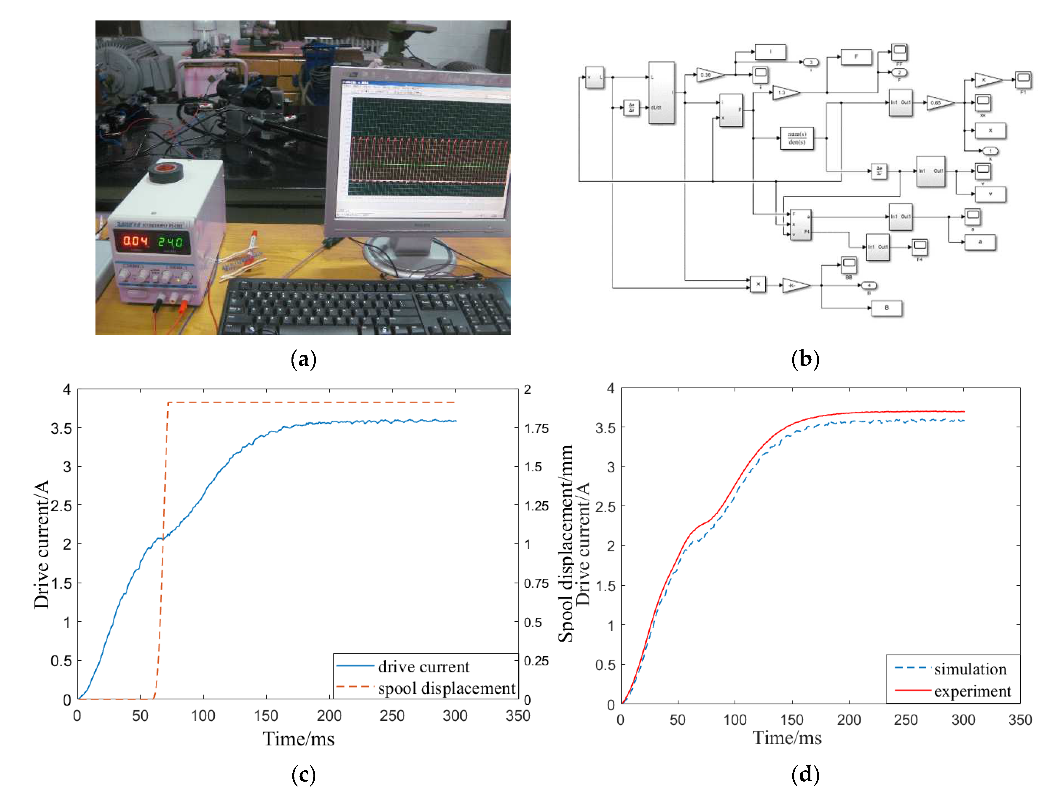
2.4. Comparison of Simulation Experiments

Based on the analysis presented above, in this subsection, the research group compares the corresponding results from a synthetic and a real experimental scenario. The research group exploited the Simulink software for the synthetic one and simulated the relationship between the drive end current of the solenoid valve and the spool displacement. For the real-world scenario, the research group utilized the 4WE10E31B/CG24N9Z5L solenoid directional valve, where the force and transient characteristics of the solenoid valve were energized and closed. The structure of the solenoid valve is presented in Figure 3. The simulation and experimental results are presented in Figure 4. The former figure illustrates the drive end current under normal conditions and the spool displacement waveform diagram when the electromagnetic directional valve is opened. The latter figure compares the drive end current simulation and experimental results.

From Figure 4, the research group observed the following:

At the initial stage of being powered on, the current could not be immediately increased to a stable value due to the self-inductance of the coil. In this process, due to the insufficient current, the electromagnetic force generated by the change in the magnetic flux in the coil was not adequate for overcoming the static friction force of the valve core and the pre-tightening force of the spring; therefore, the valve core was still in a static state.

As the current in the loop increased, the electromagnetic force generated by the coil gradually increased. When the current reached a specific value, the current curve produced an inflection point. At this point, the electromagnetic force overcame the static friction of the valve core and the preload of the spring, and the spool started to move.

When the spool started to move towards the maximum displacement, the speed of the spool continued to increase. Once the spool arrived at the maximum displacement, the spool no longer moved, and the self-inductance of the coil no longer changed. The loop current increased monotonically until it reached the maximum value.

The above analysis shows that the change in the solenoid valve drive end current can reflect the dynamic characteristics of the solenoid valve. This conclusion provides the theoretical basis for a solenoid valve fault diagnosis on the basis of drive end current detection.

2.5. Collecting Experimental Data

Our experimental setup involved a 4WE10E31B/CG24N9Z5L solenoid directional valve. The research group used the WBI342S01_0.2 electrical isolation sensor for current detection. For the data acquisition process related to the different electromagnetic states of the valve, the research group extracted the solenoid valve drive end current exploiting the NI’s USB-6356 data acquisition card. For the latter, the research group set the physical channel to AI1 and the sampling rate to 1K, and it used the WBI342S01_0.2 type of Sichuan Mianyang Weibo Electronics Co., Ltd. (Sichuan, China). A schematic of the experimental setup is illustrated in Figure 5.

During the experiments, the research group extracted the drive end currents of the solenoid valve under normal conditions, spring break, slightly stuck spool and stuck spool. In total, the research group collected 46 groups of effective current signals with the drive end current signals in various states, as presented in Figure 6. The latter figure highlights the apparent differences in the drive end current of the solenoid valve in various states. Specifically, when the solenoid valve was in the broken state of the spring, the resistance of the valve core decreased its initial point of motion advancement, and its speed and acceleration increased. When the solenoid valve was in a slightly stuck state of the spool, the resistance of the spool increased, the valve’s initial point of motion was delayed and its speed and acceleration were reduced. When the solenoid valve was in the completely stuck state of the valve core, the resistance of the valve core was too large and could not move.

3. Current Signal Feature Extraction

3.1. Time-Frequency Analysis Characteristics on the Basis of Wavelet Packet Decomposition

The three-layer wavelet packet decomposition relationship is shown in Figure 7:

$$\begin{array}{l}S=AA{A}_3+DA{A}_3+AD{A}_3+DD{A}_3\\ \hspace{1em}\hspace{1em}+AA{D}_3+DA{D}_3+AD{D}_3+DD{D}_3\end{array}$$

(8)

where S is the original signal, A and D represent the low and high frequency, respectively, and number three indicates the decomposition layers.

Information entropy is an information theory that measures the uncertainty of a random variable and quantifies the value of the information contained in the expected message [24]. Thus, the research group calculated the energy statistics on the signal after applying wavelet packet decomposition, normalized the statistic energy of each frequency band and used the normalized energy value as the characteristic value of the fault condition (Equations (9)–(12)):

$$E_{3j}^{\prime }={\displaystyle \sum _{k=1}^n{\left|x_{jk}\right|}^2}$$

(9)

$$E^{\prime }=\sqrt{{\displaystyle \sum _{j=0}^7{\left|E_{3j}^{\prime }\right|}^2}}$$

(10)

$$E_{3j}=E_{3j}^{\prime }/E^{\prime }$$

(11)

$$\begin{array}{l}{\mathrm{T}}_1=\left[\begin{array}{cccc}{E}_{30}& E_{31}& E_{32}& E_{33}\end{array}\right.\\ \hspace{1em}\hspace{1em}\left.\begin{array}{cccc}{E}_{34}& E_{35}& E_{36}& E_{37}\end{array}\right]\end{array}$$

(12)

where x_jk (j = 0:7, k = 1:n) is the amplitude of the discrete point of the reconstructed signal S3j, E’ is the energy sum of each frequency band of the signal, E_3j’ is the statistical value of each frequency band of the signal, E_3j is the t. Normalized energy of each frequency band of the signal and T₁ is the time-frequency analysis feature vector per fault type. The wavelet packet decomposition process to extract the signal energy value is presented in Figure 8.

3.2. Time-Domain Parameter Characteristics on the Basis of Principal Component Analysis

In this paper, the research group extracted 11 time-domain features, namely the average value, time-domain kurtosis, compelling value, time-domain skewness, absolute mean, waveform factor, pulse factor, threshold factor, square root amplitude, clearance factor and standard variance, defined as cx1, cx2, cx3, cx4, cx5, cx6, cx7, cx8, cx9, cx10 and cx11, respectively. These features underwent a PCA process, and the research group generated a new feature set, cy_i (i ≤ 11), with the principal component cardinality determined by the pivot contribution rate (PCR). The new feature set was utilized to form the time-domain parameter feature vector T₂:

$${\mathrm{T}}_2=\left[\begin{array}{cccc}c{y}_1& c{y}_2& \cdots & c{y}_{\mathrm{i}}\end{array}\right]\hspace{1em}\hspace{1em}\left(\mathrm{i}\le 11\right)$$

(13)

3.3. Multi-Feature Fusion Analysis

The time-frequency analysis method provides the joint distribution information of the time and the frequency domain, clearly describing the relationship between signal frequency and time. This type of analysis can detect small signals without omitting them. However, when the difference between the signal in the time and the frequency domain is not apparent, the feature vector constructed by the time-frequency analysis scheme attains insufficient recognition accuracy, presenting low credibility for pattern recognition. Time-domain analysis directly analyzes the system in the time-domain offering the most direct signal analysis method and thus has the advantages of a large amount of information, intuitiveness and accuracy. However, the actual signal is more complicated. Therefore, it is difficult to directly use time-domain analysis to reveal the signal’s frequency structure, the amplitude (or energy) of each frequency component and the relationship between the contained information and potential faults.

Spurred by the shortcomings of the time-frequency and time-domain analysis methods, this paper proposes combining wavelet packet decomposition and PCA. Specifically, the time-frequency analysis features and the time-domain parameter features of the current signal were fused, and the resulting multi-feature feature vector was then exploited for fault diagnosis.

4. Solenoid Valve Failure-Mode Recognition

SVM was developed from a linearly separable optimal classification surface and was initially used to solve the two-class classification problem, as shown in Figure 9. Its operating principle is as follows:

In the data set, a hyperplane is constructed, where the largest w and b are chosen to maximize the edge; therefore, the distance between the hyperplane and any nearest training data point is the largest, and the points with y_i = 1 and y_i = −1 separate.

$$w\cdot x+b=0$$

(14)

Currently, several algorithms extend the classic two-class SVM to a multi-class problem, with the latter roughly divided into two categories. The first one constructs a series of two-class classifiers and combines them to achieve multi-classification. In contrast, the second type, entitled S-type, calculates the parameters for the multiple classification planes and merges them into an optimization problem utilizing a “one-time” optimization strategy to achieve multi-classification [25]. Given that the training sample cardinality is relatively small, the requirement for training speed is not high, and thus, the S-type approach is more accurate. Hence, in this work, the research group exploited the S-type method both for classification and recognition. It is worth noting that, for the S-type of problems, Weston and Watkins [26] proposed a method to solve all hyperplanes at once.

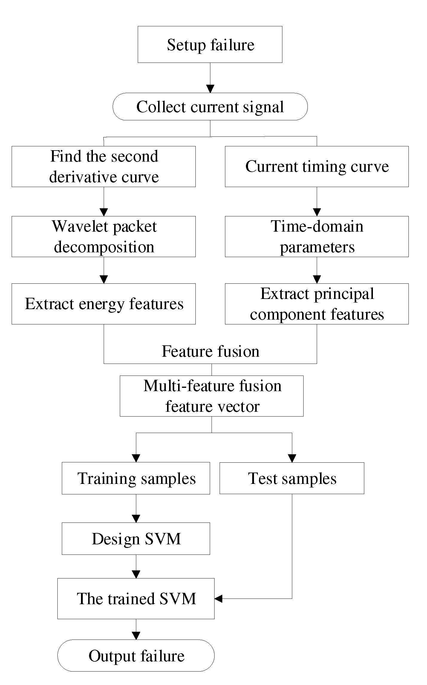
The fault identification process relying on SVM is divided into two stages:

(1)

Training modeling: First, the information of the system under different fault types is obtained utilizing sensor measurement. Then, data processing is performed on the information to extract a feature vector and to form a training sample pair between the feature vector and its corresponding fault type, to ultimately establish the relationship between the sample and the fault type. This relationship is then exploited to train the SVM.

(2)

Model prediction: The feature information to be diagnosed is input into the trained SVM, and the latter’s output presents the fault diagnosis classification.

4.1. Input and Output Design

The SVM input is generally the eigenvector of the sample. In this paper, the research group utilized the signal’s time-domain parameters and the information energy of the time-frequency curve as eigenvalues and constructed the eigenvectors on the basis of time-frequency and time-domain analyses. This article classifies the four states of a solenoid valve, namely normal spool, broken spring, stuck spool and slightly stuck. The different states of the solenoid valve are numbered as 0 for normal spool, 1 for spring break, 2 for spool stuck, and 3 for spool slightly stuck.

4.2. SVM Design

Multi-classification SVMs mainly include four types: C-SVC, υ-SVC, ε-SVR and υ-SVR. C-SVC and υ-SVC are utilized for the label classification of sample vectors, and ε-SVR and υ-SVR perform regression on the label value of the sample vector. In this paper, the research group exploited the C-SVC on the basis of the RBF to identify and classify the state of the solenoid valve.

5. Fault Diagnosis Example of an Electromagnetic Reversing Valve

5.1. Fault Diagnosis Process

The suggested solenoid valve fault-diagnosis method involves the following stages. Initially, collect the drive end current signals under four typical solenoid valve operation conditions, i.e., normal, spring breakage, spool jamming, and slight spool jamming. Then, use the wavelet packet decomposition and energy statistics to extract the time-frequency analysis characteristics of the signal, which are then input to a PCA scheme to obtain the new time-domain parameter characteristics of the signal. After that, fuse the time-frequency analysis features with the new time-domain parameter features, and finally, use the optimal SVM to classify and identify the solenoid valve fault. The diagnosis pipeline is presented in Figure 10.

5.2. Time-Frequency Analysis of a Multi-State Current Signal

This experiment performs time-frequency analysis to the second-order change rate of the current value with the corresponding results shown in Figure 11.

The research group extracted the signal of eight frequency components, ranging from low to high frequency, utilizing a three-layer wavelet packet decomposition (Figure 12), from which the research group derived the following observations. For standard valves, the energy amplitude fluctuations in a single frequency band were small, and the energy values of the sixth and eighth frequency bands were higher. For the spring rupture valve, it can be seen from Figure 12c–h that, in the third to eighth frequency bands, the energy amplitude in a single frequency band fluctuated significantly, the energy amplitude in the early stage was significantly more extensive and the fifth, sixth and eighth frequency band energy values were higher. For the spool stuck valve, the energy amplitude in a single frequency band fluctuated significantly, the energy amplitude in the later stage was significantly greater, and the energy value of the fifth, sixth and eighth frequency bands were higher. For the slightly stuck spool valve, the amplitude fluctuation in a single frequency band was slight, the energy amplitude in the later period was slightly higher and the energy values of the sixth and eighth frequency bands were higher.

5.3. Time-Domain Analysis of a Multi-State Current Signal

In this trial, the research group considered 11 parameters: the average current value, time-domain kurtosis, effective value, time-domain skewness, absolute mean value, form factor, pulse factor, threshold factor, root square amplitude, clearance factor and standard deviation. On these parameters, the research group applied PCA to reduce the parameter vector dimensionality and calculated the contribution rates of the different principal components, as presented in

Table 1. Contribution rate of each principal element.

Principal Element	Contribution Rate (%)
1	60.0411
2	29.1488
3	9.0540
4	1.6772
5	0.0659
6	0.0071
7	0.0051
8	0.0005
9	0.0002
10	0.0001
11	1.21 × 10−5

.

The research group determined the number of pivots by the Cumulative and Percentage Method of Pivot Contribution Rate (PCR). From the results of Table 1, the research group concluded that selecting the first four pivots afforded a cumulative contribution rate of 99.9211%. The corresponding coefficients of the first four pivots are shown in

Table 2. Coefficients of the first four principal components.

	1	2	3	4
p1	−0.3333	0.2689	0.1710	0.1703
p2	−0.2795	−0.3300	−0.2900	0.5124
p3	−0.2594	0.4140	0.0356	0.1565
p4	0.2871	0.2245	0.5244	−0.3011
p5	−0.3333	0.2687	0.1719	0.1717
p6	0.2469	0.3678	−0.4031	−0.0773
p7	0.3537	0.0989	0.3041	0.5200
p8	0.3529	0.2034	−0.0267	0.4869
p9	−0.3500	0.1216	0.3778	0.0651
p10	0.3101	−0.3042	0.2449	0.2126
p11	0.1439	0.4806	−0.3499	0.0305

.

Let the first four principal components be cy₁, cy₂, cy₃ and cy₄; hence:

$$c{y}_i={\displaystyle \sum _{j=1}^{11}c{x}_j\cdot p_j}\hspace{1em}\hspace{1em}\left(i=1,2,3,4\right)$$

(15)

Then, the research group constructed the time-domain parameter feature vector:

$${\mathrm{T}}_2=\left[\begin{array}{cccc}c{y}_1& c{y}_2& c{y}_3& c{y}_4\end{array}\right]$$

(16)

and the research group combined the time-frequency analysis feature with the time-domain parameter feature to construct a new feature vector:

$$\begin{array}{l}\mathrm{T}=\left[\begin{array}{cccccc}{E}_{30}& E_{31}& E_{32}& E_{33}& E_{34}& E_{35}\end{array}\right.\hspace{1em}\hspace{1em}\\ \hspace{1em}\left.\begin{array}{cccccc}\hspace{1em}{E}_{36}& E_{37}& c{y}_1& c{y}_2& c{y}_3& c{y}_4\end{array}\right]\end{array}$$

(17)

5.4. Result Analysis

The research group used the RBF-based C-SVC to identify and classify the fused feature vectors, with the corresponding recognition results illustrated in Figure 13. The results indicate that, when the feature vector is constructed by fusing the time-frequency analysis features and the time-domain parameter features, the training accuracy rate is 100%, the testing accuracy rate is 100% and the five-fold cross-validation accuracy rate is 92.11%. The training process of the SVM is a process of continuous optimization, where the feature vector samples are input into the SVM for training, and after 1000 epochs, the accuracy rate tends to be stable. The trials show that using C-SVC on the basis of RBF can accurately identify the four states of the electromagnetic directional valve (normal valve, spring broken, spool stuck and slightly stuck spool).

To support the findings, the research group challenged the performance of the method against [1], which employed a BP neural network, and [27], which utilized time-frequency analysis to identify the failure mode. The training target error and training times of BP neural network were set by the grid search method. The corresponding results are presented in Figure 14. The latter figure reveals that the BP network recognition accuracy rate was 84.78%, and the C-SVC recognition accuracy rates on the basis of time-frequency analysis and on the combination of time-frequency analysis and time-domain analysis were 91.3% and 100%, respectively.

6. Conclusions

This paper studies the problem of solenoid valve fault diagnosis on the basis of the current detection method at the driving end. The research group analyzed the characteristics of the drive-end current under four conditions: normal solenoid valve spool, spring broken, spool stuck and slightly stuck spool. The proposed method selects the solenoid valve drive end current value and its second-order rate of change curve as the characteristic curve and constructs a multi-feature fusion solenoid valve state eigenvector on the basis of a three-layer wavelet packet decomposition and PCA. Then, the research group reconstructed the original signal using the energy-fault method to calculate the energy statistics on the reconstructed frequency bands and employed the statistically obtained energy value of each frequency band as a feature vector. Finally, the research group designed C-SVC to perform pattern recognition on the state of the solenoid valve and to compare the performance of the method against the BP neural network and C-SVC on the basis of time-frequency analysis.

The significant findings of the research are:

(1)

Using the solenoid valve drive end current value and its second-order rate of change curve as the signal’s characteristic curve, it is possible to extract characteristic vectors with apparent differences.

(2)

The C-SVC pattern recognition method on the basis of RBF has an accuracy rate of 91.3% and a cross-validation accuracy rate of 50%.

(3)

The BP neural network used to perform pattern recognition and to exploit the multi-feature fusion on the four states of the solenoid valve manages an accuracy rate of 84.78%.

(4)

The proposed C-SVC method on the basis of RBF exploiting multi-feature fusion on the four states of the solenoid valve manages an accuracy rate of 100% and a cross-validation accuracy rate of 92.11%. Specifically, both the training and testing accuracy rates are 100%, highlighting the method’s capability to correctly classify all four states of solenoid directional valve spools, i.e., normal, spring broken, spool stuck and spool stuck slightly.

There are still some shortcomings in this paper: the support vector machine belongs to machine learning and is a method on the basis of mathematical statistics, which lacks the physical interpretation of experimental results. We plan to analyze the interpretability of this method in the future from the perspective of the failure mechanism.