Multi-Classification of Motor Imagery EEG Signals Using Bayesian Optimization-Based Average Ensemble Approach

Abstract

Motor Imagery (MI) classification using electroencephalography (EEG) has been extensively applied in healthcare scenarios for rehabilitation aims. EEG signal decoding is a difficult process due to its complexity and poor signal-to-noise ratio. Convolutional neural networks (CNN) have demonstrated their ability to extract time–space characteristics from EEG signals for better classification results. However, to discover dynamic correlations in these signals, CNN models must be improved. Hyperparameter choice strongly affects the robustness of CNNs. It is still challenging since the manual tuning performed by domain experts lacks the high performance needed for real-life applications. To overcome these limitations, we presented a fusion of three optimum CNN models using the Average Ensemble strategy, a method that is utilized for the first time for MI movement classification. Moreover, we adopted the Bayesian Optimization (BO) algorithm to reach the optimal hyperparameters’ values. The experimental results demonstrate that without data augmentation, our approach reached 92% accuracy, whereas Linear Discriminate Analysis, Support Vector Machine, Random Forest, Multi-Layer Perceptron, and Gaussian Naive Bayes achieved 68%, 70%, 58%, 64%, and 40% accuracy, respectively. Further, we surpassed state-of-the-art strategies on the BCI competition IV-2a multiclass MI database by a wide margin, proving the benefit of combining the output of CNN models with automated hyperparameter tuning.

1. Introduction

Brain Computer Interface (BCI) is a revolutionary technology, that permits direct communication with the brain through computers, without the involvement of peripheral nerves or muscles. This happens by sensing the human brain signals and translating them into commands-based applications that are mainly designed to help disabled individuals suffering from motor diseases and congenital conditions, such as Kennedy’s Symptoms, Progressive Bulbar Palsy (PBP), Muscular dystrophy (MD), or locked-in syndrome, to communicate with the external world.

The electroencephalogram is one of the most effective non-invasive methods for studying the electrophysiological dynamics of the brain. It is widely used in BCI-based applications [1] because it is portable, easy to use, inexpensive, and it has a high temporal resolution. Regardless of having a very low signal-to-noise ratio and its low spatial resolution, it is still considered the best choice for collecting human brain motor cortex signals among all other existing options, such as Magnetoencephalography (MEG), Positron Emission Tomography (PET), or functional Magnetic Resonance Imaging (fMRI) [2], which are more complicated to employ.

MI-based EEG is a commonly used approach within BCIs. It is a cognitive process that does not require any prior stimuli. It relies completely on the subject imagination of an action without physically performing it. This helps generate a signal similar to that of body movement [3]. In general, brain signals are time varying, and subject specific [4], making MI-EEG feature extraction and classification difficult, especially for conventional Machine Learning (ML) algorithms [5] that involve a handcrafted signal processing pipeline and a long training time to learn significant features. Moreover, traditional ML is domain specific. This reduces its common potential application in the general context of rehabilitation-related technologies. As a result, they largely fail to satisfy the growing level of performance needed from real-life-based BCI applications.

Deep Learning (DL) algorithms achieved good results dealing with time series and other traditional ML algorithm limitations. One of the best Deep Neural Networks (DNN) algorithms is CNN [6]. It does not require data pre-processing nor feature extraction prior to classification. The CNN classifier manages raw EEG data analysis successfully in several application domains and has achieved a satisfying result [7,8]. However, the complex nature of the signal and the implementation of more advanced CNN architectures demand an optimal hyperparameter deployment to decrease the training time and increase the learning rate. Hyperparameter selection is an essential step in building any CNN model. The manual tuning of those parameters may lead to uncertain results as it depends on the intuition of the user. The choice of the right combinations is time consuming and demands expert knowledge. This limitation can be solved by considering optimization algorithms that help reach the global optima of a given CNN by choosing the appropriate set of values of the hyperparameters in a given space in less time efficiently and automatically.

This paper’s contributions are as follows: (1) As far as we know, it is the first time, the concept of Average Ensemble of optimized CNNs is applied to the EEG MI movement classification problem, achieving a high level of performance. (2) Our proposed approach outperformed the recent methods in the BCI competition IV-2a 4-class MI database [9] by a significant margin. (3) The proposed approach’s performance is extensively evaluated by comparing it to five traditional ML algorithms (Linear Discriminate Analysis [10], Support Vector Machine [11], Random Forest [12], Multi-Layer Perceptron [13], and Gaussian Naive Bayes [14]). (4) The optimum hyperparameters are determined automatically by employing BO.

The classification performance of MI-EEG signals is an important part of building a strong and reliable BCI application. Many researchers, therefore, investigated different approaches seeking good results. Javeria et al. [15] used Support Vector Machine, Naïve-Bayesian Parzen-Window (NBPW), and K-Nearest Neighbour (KNN) algorithms to train and classify upper limb MI tasks and rest. Features were extracted by carrying out Common Spatial Pattern and Linear Discriminate Analysis for feature extraction. Since not all of the extracted features are necessary for classification, the optimal features are selected by using the Sequential Backward Floating Selection (SBFS) method. Two datasets were employed to assess the algorithm’s performance. Their proposed method achieves an accuracy of 86.50% on the Wet Gel Electrodes dataset and 60.61% on the Emotive Epoch Headset. Bhattacharyya et al. [16] classified upper limb movement using raw EEG signals acquired from the BCI competition-II 2003 dataset [17]. Unreduced features along with reduced features were tested on the following classifiers: Linear Discriminate Analysis, Quadratic Discriminant Analysis (QDA), KNN, Support Vector Machine, Radial Basis Function (RBF), and Naive Bayesian (NB) classifier. Consequently, the best results were achieved by Support Vector Machine, reaching an accuracy of 82.14% in both scenarios, whilst KNN’s performance improved with reduced features. Wahid et al. [18] used EEG signals from 40 healthy people and four ML classifiers, including Support Vector Machine, Linear Discriminate Analysis, Random Forest, and KNN, to identify foot and hand movement tasks. Common Spatial Pattern features were retrieved from several window widths, ranging from 0.3 s to 2 s. The findings demonstrate that with 2 s window sizes and nine votes, the KNN can reach 78.9%. The ranking study utilizing both accuracy and area under the curve data demonstrate that the Random Forest method can consistently perform well with varying window sizes and amounts of votes. Yang et al. [19] explored the effectiveness of CNN for multi-class MI-EEG data classification. They constructed augmented Common Spatial Pattern features employing pair-wise projection matrices, which deal with various frequency ranges. There are eight levels of frequency bands, with 4 Hz and 40 Hz being the starting and ending frequencies, respectively. The width of each band is selected as (3 4 7 8 11 12 13 15) Hz and the widths of each window shift are (2 2 4 5 6 6 5 5). In total, there are 60 frequency bands. Furthermore, they presented a frequency complementary feature map selection approach that limits the reliance across frequency bands, attaining an averaged cross-validation accuracy of 69.27%. Their findings show that CNN can acquire deep and discriminant structural features for EEG classification without depending on handcrafted features (handcrafted features are those that are manually engineered). Cheng et al. [20] employed a cascade of one-dimensional convolutional neural networks and fully connected neural networks (1D-CNN-FC) with a cooperative training method to classify background EEG and MI-EEG. Six convolutional layers and two fully connected layers comprise the 1D-CNN-FC cascade. They compared their proposed cascade to the traditional strategy for motor imagery-BCI, which included Support Vector Machine for classification and Common Spatial Pattern for feature extraction. Their experiments compare three classification tasks: Firstly, to classify pure imagery from background EEG, secondly, transitional imagery from background EEG, and lastly, to separate both pure and transitional imagery from background EEG using a joint training scheme, considering pure and transitional imagery signals as the same class. The cooperative training method outperformed traditional training in their experiments. Abbas et al. [21] presented a framework in which the covariance maximization method is adopted for discriminating inter-class data and this technique uses Fast Fourier Transform Energy Maps (FFTEM) to convert 1D data into 2D data and select features. FFTEM is used as a feature selection method, which exploits both the spectral and energy information hidden in EEG data. It is applied to the discriminative features obtained from Common Spatial Pattern filters to compute energy maps corresponding to frequency bands and EEG channels. These energy maps are used to train the CNN classifier. It was necessary to convert 1D data to 2D as they were using 2D CNN. Their proposed classification system achieved a mean kappa value of 0.61%. Sakhavi et al. [22] applied a CNN architecture for classification as well as a novel temporal representation of the data. Their new representation is developed by adjusting the filter-bank technique, and the CNN is constructed and optimized for the representation accordingly. On the BCI competition IV-2a dataset, their approach surpassed the recent methods in the literature by a 7% improvement in average subject accuracy. Zhao et al. [23] suggested a three-dimensional visualization approach as well as a multi-branch three-dimensional CNN to solve MI classification challenges. Their three-dimensional CNN representation is created by converting EEG data into a series of 2-dimensional arrays that maintain the sampling electrodes’ spatial distribution. Their innovative experiments demonstrated that the introduced method achieves state-of-the-art classification kappa score levels and considerably surpasses other classifiers by a 50% reduction in various subjects’ standard deviation. Furthermore, they proved that the multi-branch architecture may reduce overfitting when the size of the dataset is insufficient. Liu et al. [24] presented a new semi-supervised cartesian k-means for MI-EEG classification. They employed CNN architectures that had been pre-trained on MI examples to produce deep features, which they then used to classify MI data. Deep features are the high-level features that are extracted by the feature extraction block of the CNN. Their experimental results show that their suggested strategy outperforms other comparable algorithms. Deng et al. [25] presented the Temporary Sparse Group Lasso (TSGL) EEGNet neural network algorithm, which has superior efficiency on the MI-EEG and is easily interpretable. Their suggested algorithm was improved on the basis of a well-recognized DL model, known as EEGNet, and it was optimized using the traditional ML approach. Their experimental findings indicated that their approach obtained an average accuracy of 81.34% and a kappa of 75.11% on the BCI Competition IV 2a dataset [9]. Zümray Dokur et al. [26] evaluated the influence of the augmentation procedure’s effect on the MI-EEG’s classification performance rather than employing a previous transformation (Common Spatial Pattern). Furthermore, they redesigned the DNN topology to improve classification results, reduce the number of nodes in the architecture, and employ fewer hyperparameters. Moreover, they examined these enhancements on datasets from BCI competitions in 2005 and 2008, with two and four classes, respectively, and found that the augmentation had a significant influence on the average performance.

The above-cited techniques remain relatively practical, due to their drawbacks, and functioning mode. BO algorithm overcomes those limitations due to its processing manner [27]. The BO concept is based on the assumption function, which holds predicted values, whereas the acquisition function helps predict the next point until reaching the global optimum. The posterior probability related to the Gaussian distribution of the unknown optimized objective function is obtained from prior information and sample data. It is effective and precise on complex training and high-dimensional data. Further, it reduces time cost and delivers accurate results. Wu et al. [28] studied the effect of hyperparameter tuning on an ML algorithm employing BO with Gaussian Process (GP). They used the same dataset on other optimization algorithms, such as Random Forest and multi-grained cascade forest. As a result, the BO algorithm outperformed the other methods. Hengjin et al. [29] aimed to optimize an EEG-based CNN classifier for online E-health programs, which needs high precision and inexpensive time cost to manage the brain dynamics simulations. They employed the BO algorithm on time series data in a fashioned manner. They sliced up the hyperparameters into groups. Each group was optimized under the same conditions in the same space but separately. Then, the selection of the most optimized values is conducted through a matrix based on Markov Chain. The employment of the BO contributed significantly on building a robust CNN model and successfully handling EEG data. Brenda et al. [30] used two different techniques for MI-EEG classification on the BCI competition IV dataset 2a [9] and eight other pieces of EEG data [30]. On both methods, feature extraction was executed by a Filter Bank Common Spatial Pattern (FBCSP). After frequency band selection, the matrix containing salient features is fed into previously optimized conventional CNN to perform binary classifications of all classes. The same processed data are fed into four more evolutive CNNs classifiers. As a result, the accuracy improved.

As can be noticed, individual models were used in the majority of EEG signal classification investigations. In our study, we focused on merging the optimum results of three robust CNNs trained separately. Besides that, none of the aforementioned studies used BO in conjunction with Ensemble Learning (EL) approaches. Consequently, they failed to meet near-perfect performance, which is unacceptable in the clinical context.

This paper builds upon EL, DL, and BO to accomplish three major goals:

• Design an efficient classification system by merging the top three best CNNs generated by the help of BO addressed for BCI-based rehabilitation uses.
• Obtain competitive findings using BCI IV-2a competition data by reaching high levels of Precision, Recall, F1-score, Accuracy, and Kappa.
• Highlight the significant contribution of BO and checkpoint call back techniques on boosting the performance of CNN on MI data.

The paper is structured as follows: Section 2 discusses the proposed BO-based Average Ensemble approach for the classification of four EEG tasks, including the left hand, right hand, tongue, and feet. Section 3 illustrates the experimental results and a comparison of state-of-the-art strategies. Lastly, Section 4 concludes the paper.

2. Materials and Methods

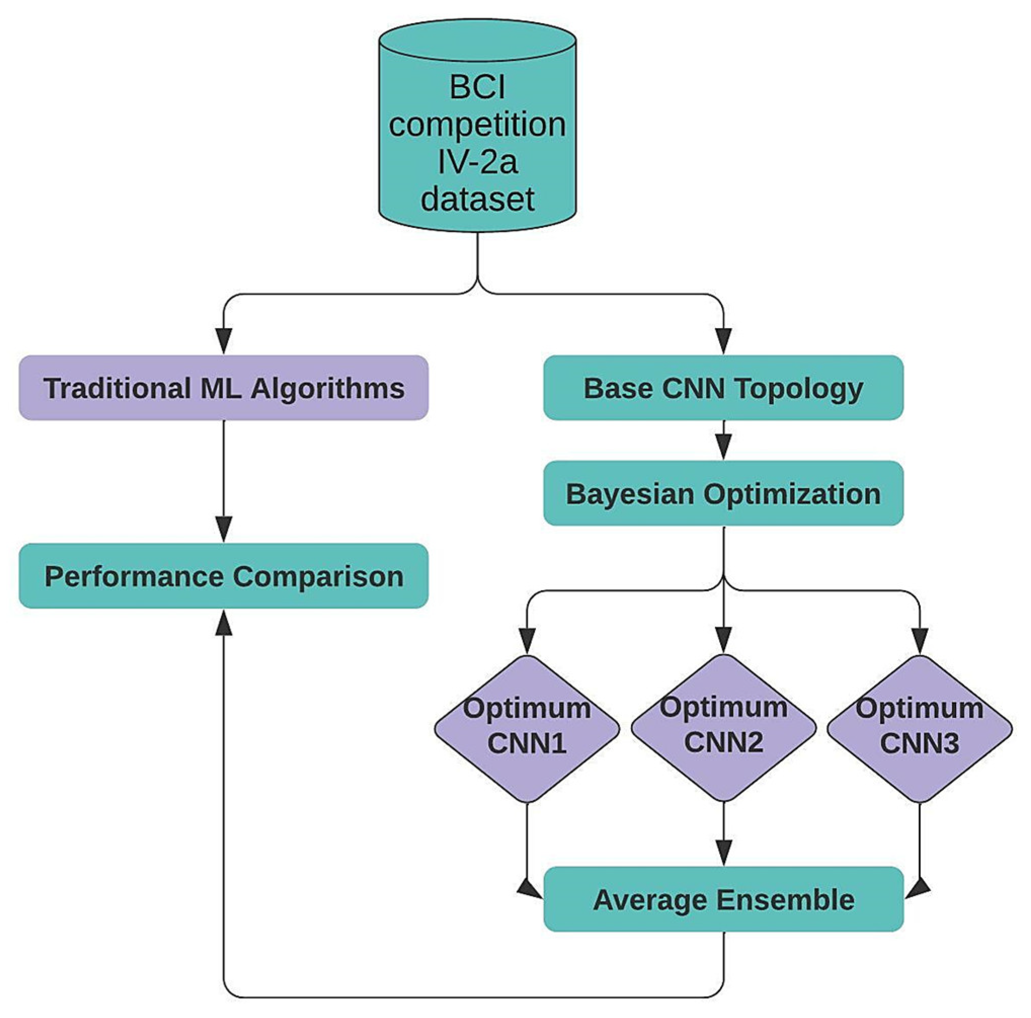
This section describes the proposed approach for EEG data multi-classification. First, we present our target dataset. Next, we introduce the proposed one-dimensional CNN topology. Then, we discuss how BO can be used to select the optimal hyperparameters. After, we describe the Average Ensemble method, which was used to combine the three top-generated CNNs from the BO stage. Last, we compare our Ensemble model to five traditional ML algorithms. Figure 1 depicts the overall flow of the proposed framework.

2.1. Data Acquisition

In this article, we used the open-for-use BCI Competition IV 2a dataset 2008 from Graz university [9]. It contains 9 subjects’ signals recorded for left hand, right hand, tongue, and feet. Each subject’s data were collected in two days. Each day is one session. Each session contains a total of 6 runs each including 12 trials for every imagined movement. Subjects take a short pause between the runs. To start the recording, the participants sat in a comfortable chair in front of a digital screen with arrows indicating the task of imagination. Each arrow stays for about 1.25 s. Before the beginning of each trial, a cross appears for 2 s on the screen along with a beep to signal the beginning of the trial. The duration of each MI trial after the cue is 3 s. The cue in the task was in the form of an arrow. The BCI Competition 2a dataset was recorded using 22 electrodes with a sampling rate of 250 Hz and a sensitivity of 100 µV. Then, a bandpass filtered between 0.5 Hz and 100 Hz was applied. To eliminate the noise, a 50 Hz notch filter was used. A representation of the BCI Competition IV-2a’s synchronicity is shown in Figure 2.

Data pre-processing is a commonly applied step in a majority of signal processing-related studies. It helps clean the data from environmental and physiological artifacts and discard bad trials [31]. Furthermore, the application of filters helps reshape the data according to the study context and needs. However, in our case study, we are using BCI Competition IV dataset 2a which is already pre-processed. We are, therefore, not willing to apply any further modification since our methodology is based on an end-to-end automated pipeline for MI classification with CNN. CNNs are well-known for their capacity to handle raw EEG data and extract features. Further, the classification is executed automatically. The eye movement data collected from Electrooculography (EOG) channels are not considered in this experiment.

2.2. The Proposed Base CNN Architecture

In this paper, we first created a base CNN topology before performing hyperparameter optimization. Our proposed 1D-CNN has 2 main blocks (2 convolutional, 2 batch normalization, and 2 max-pooling layers), and a classification block (4 dense and 3 dropout layers). The architecture of the proposed base CNN approach is depicted in Figure 3.

In each convolution layer, we used 64 convolution filters, 3 filter sizes, and 1 time step. As a fuzzy filter, convolution layers improve the features of original signals and eliminate noise. A convolution operation takes place between the upper layer’s feature vectors and the current layer’s convolution filter. Finally, the activation function returns the outcomes of convolution calculations. Equation (1) shows the outcome of the convolution layer:

$$X_j^l=f({\displaystyle \sum }_{i\in M_j}{X}_j^{l-1}\times W_{ij}^l+b_j^l)$$

(1)

where $M_j$ denotes the current neuron’s receptive field. $X_j^l$ represents the characteristic vector for the $l\mathrm{th}$ layer’s $j\mathrm{th}$ convolution filter. $f$ means a nonlinear function. $W_{ij}^l$ represents the bias coefficient assigned to the $l\mathrm{th}$ layer’s $j\mathrm{th}$ convolution kernel.

We utilized Batch Normalization [32] after each convolutional layer to enhance performance results and accelerate training convergence. It is accomplished by normalizing each feature at the batch level during training and then re-scaling later with the entire training data in mind. Each mini-batch’s dimension is transformed as shown in Equation (2), where $Var\left[x^{\left(k\right)}\right]$ and $E\left[x^{\left(k\right)}\right]$ represent the variance and the mean of $k\mathrm{th}$ scalar feature, respectively. The numerical stability is improved by a minor constant $ϵ$.

$${\widehat{x}}^{\left(k\right)}=\frac{x^{\left(k\right)}-E\left[x^{\left(k\right)}\right]}{\sqrt{Var\left[x^{\left(k\right)}\right]+ϵ}}$$

(2)

The learnable parameters $\beta$ and $\gamma$ are introduced through Batch Normalization. The transformation of each layer is described in Equation (3).

$$BatchNormalization\left(x^{\left(k\right)}\right)={\gamma }^{\left(k\right)}\times {\widehat{x}}^{\left(k\right)}+{\beta }^{\left(k\right)}$$

(3)

Pooling is a sublayer of a CNN that introduces non-linearity by amalgamating nearby values’ feature into one, using a specific operator. The most common options are average-pooling and max-pooling. We chose max-pooling [33] for this study. As the point after pooling, the maximum value of the pool area is used. This minimizes the output’s spatial size, reducing the model’s computational complexity. We employed 1D max pooling with a stride size of 1 and a pooling size of 2.

In order to generate the final output, dense layers were applied to produce an output equal to the number of classes (this study takes four classes into account). We selected $y=fc\left(x,w,b\right)$ to represent the function performed by the dense layer, where $y$ means the output, $x$ denotes the input to the dense layer, $w$ represents the weight matrix, and $b$ describes the bias. The input $x$ includes $Z$ features. The component $x_i$ represents feature $i$. It is worth noting that $w$ contains dimension $Z\times A$, where $A$ reflects the $y$’s dimension. It works with a vector $x$ to generate the component $j$ in $y$, as shown in Equation (4).

$$y_j={\displaystyle \sum }_i{w}_{ij}{x}_i+b_j$$

(4)

To prevent over-fitting and improve generalization, we used the Dropout [34] technique between dense layers. Dropout offers regularization by removing a portion of the previous layer’s outputs.

It should be noted that this step did not include:

• The dropout rate.
• The activation functions.
• The number of nodes in the first three dense layers.

These are among the hyperparameters that will be used as inputs for BO in the next subsection.

2.3. Hyperparameter Optimization

Tuning hyperparameters is an optimization problem with an unknown objective function. As can be seen in Equation (5), where $x$ denotes a hyperparameter setting, $x_{opt}$ means the best choice and $f$ represents performance.

$$x_{opt}=\underset{x\in X}{argmax}f\left(x\right)$$

(5)

There is a range of methods that can be used to accomplish this. Grid Search [35], for example, is a method for searching exhaustively over a portion of a hyperparameter space for a certain algorithm. The number of parameter combinations will grow exponentially as additional hyperparameters are introduced. As a result, the procedure will take a long time to complete. Random Search [35] is another method for locating valuable hyperparameters. Random Search, unlike Grid Search, tries out different combinations of parameters at random. When computing, this causes a high variance. These two approaches are unable to learn anything from the assessed hyperparameter sets during the optimization procedure.

In this experiment, an efficient strategy known as BO [36] is adopted to select the optimum hyperparameters. BO incorporates previous knowledge about the objective function and updates posterior knowledge, increasing accuracy and reducing model loss. The optimization is carried out in accordance with Bayesian Theorem [37], which is enshrined in Equation (6), where $M$ denotes the model and $O$ denotes the observation.

$$P(M|O)=(P(O|M)P\left(M\right)/P\left(M\right)$$

(6)

where $P\left(M\right)$ describes the prior probability of $M$, $P\left(M|O\right)$ is $M$’s posterior probability given $O$, and $P(O|M)$ is $O$’s likelihood given $M$. By using BO, one can find the objective function’s minimum on a bounded set. The CNN model with additional evaluations for the objective function is adequate for making the right choices. By reducing the error in validation, BO leads to optimal CNNs in the current study.

The first critical step in the BO process is to use a Posterior distribution with a GP to update the prior Function F results. GP provides a set of observed previous possible values transformed directly into posterior probabilities on the functions. This scenario allows us to apply GP in our multi-classification problem. The next step is to use an acquisition function to pick the optimum point for F. Following that, BO identifies the suggested sampling points as determined by the acquisition function. The Expected Improvement (EI) acquisition function is used at the points where the objective function is maximum and the location where the uncertainty of the prediction is high. The mathematical representation of EI function is shown in Equation (7), where $MSP$ denotes the sample points’ mean, $OFH$ means the Optimization Function at the highest point. The optimization function has a search space limitation represented as $L$. The Cumulative Distribution, denoted by $CD$, takes into account all of the points up to the point sample under Gaussian distribution.

$$Expected Improvement=\left(\left(MSP-OFH\right)-L\right)\left(CD\right)$$

(7)

In order to obtain results in the validation set, it is essential to use an objective function. The critical step after that is to update the Gaussian distribution network. Several iterations of this process are completed in order to tune the validation set for creating optimized hyperparameters that work best for our classification problem. In this paper, 60 iterations were performed. The flow of BO algorithm related to our proposed CNN network is summarized in Figure 4.

The hyperparameters chosen for optimization in this experiment are:

The activation function for the convolutional layers and the first three dense layers.

• The dropout rate.
• The number of nodes in the first three dense layers.
• The optimizer.
• The batch size.

For each of these hyperparameters, the valid search ranges are predefined. “ReLU, SELU, Tanh, ELU, and Sigmoid” are the activation functions specified for the convolutional layers and the first three dense layers. ReLU is a popular activation function in CNN. It applies a threshold function to every input element, setting anything less than 0 to 0. SELU is an activation function that promotes self-normalization. SELU network neuronal activations naturally settle to a 0 mean and unit variance. Tanh is used to estimate or discriminate between two classes; however, it only transfers negative inputs into negative quantities ranging from −1 to 1. ELU is a neural network activation function. ELU, unlike ReLU, has negative numbers, allowing it to bring mean unit activations closer to 0, similar to batch normalization, but with less computing effort. Sigmoid is a type of non-linear activation function that is commonly employed in feedforward neural networks. It is a probabilistic method to play an important factor that ranges from 0 to 1. Thus, when we need to make a choice or estimate an outcome, we utilize this activation function since the range is the smallest, so prediction is more correct.

The dropout rate is set between 0 and 0.5. The number of nodes in the first three dense layers has a lower bound of 32 and an upper bound of 1024. The optimizers specified are Nadam (Adam with Nesterov momentum), RMSProp (root means square propagation), Adam (adaptive moment estimation), SGD (stochastic gradient descent), and AdaMax (an Adam variant). The low and high of the batch size are 1 to 128.

Table 1. Hyperparameter setting.

Hyperparameters	Range to Probe
Activation function	ReLU–SELU–Tanh–ELU–Sigmoid
Dropout rate	0 to 0.5
Number of nodes in the first dense layer	32 to 1024
Number of nodes in the second dense layer	32 to 1024
Number of nodes in the third dense layer	32 to 1024
Optimizer	Nadam–RMSProp–Adam–SGD–AdaMax
Batch size	1 to 128

lists the hyperparameters considered in the BO experiment, as well as the search space for each hyperparameter.

2.4. Ensemble Learning (EL)

In ML, EL is defined as the training of several models, known as weak learners, and the merging of their predictions to generate improved results. It allows us to merge all of these models to obtain a single excellent model that is based on insights from most or all of the training set [38]. The fact that there is no limit to the number of weak learners that can be used is an intriguing feature of EL. It could range from as few as two to as many as ten weak learners. EL can be used in a variety of ways to enhance overall performance, including averaging, weighted averaging, max voting, and many others.

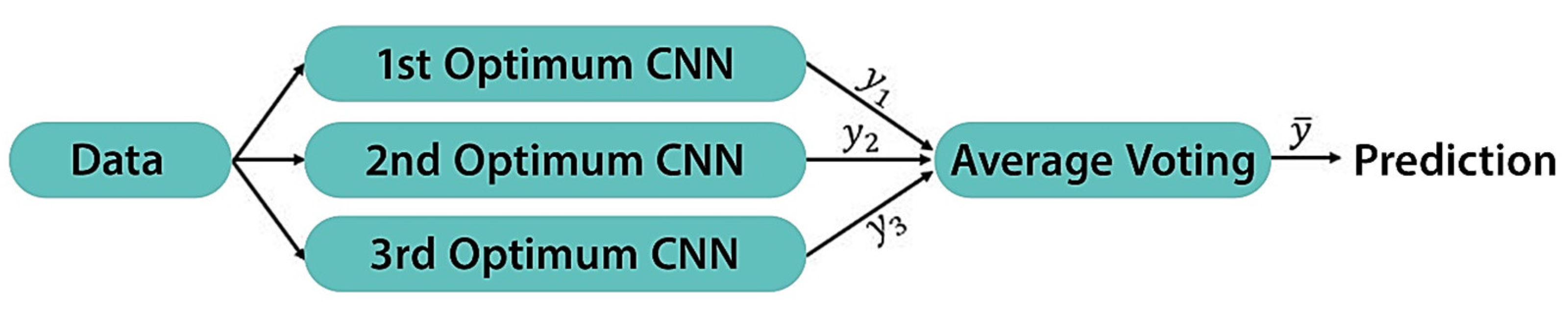
The motivation behind employing the EL approach is to improve the overall efficiency of the top three optimum models generated by BO. Further, it eliminates the possibility of weak learners focusing on local minima. In this paper, we utilized the Average Ensemble method. With this method, each prediction on the test set is averaged, and finally the prediction is derived from the average prediction model. Each of the three weak learners make an equal contribution to the overall prediction as shown in Equation (8).

$$\overline{y}\left(\mathrm{x}\right)=1/3{\displaystyle \sum }_{m=1}^3{y}_m\left(x\right)$$

(8)

The specific steps of this method can be described as follows: (1) generate three weak learners (top three optimum models) from the BO experiment, (2) train them separately from scratch on the same dataset, and (3) merge these weak learners by averaging their predictions ($y_1$,$y_2,y_3)$ for each sample of our dataset to calculate $\overline{y}$. An illustration of the structure of the proposed Average Ensemble method is displayed in Figure 5.

2.5. Traditional ML Algorithms

In this experiment, we picked five traditional ML algorithms (Linear Discriminate Analysis, Support Vector Machine, Random Forest, Multi-Layer Perceptron, and Gaussian Naive Bayes) to compare their performance with our proposed Average Ensemble approach. We trained these algorithms on the same dataset in order to offer a fair performance evaluation. Note that the hyperparameters of the five traditional ML algorithms are not optimized in our experiment. We used Scikit-learn [39] Python Package to build these algorithms and we trained them with the default hyperparameters provided in this Package.

2.5.1. Linear Discriminate Analysis (LDA)

LDA [10] is a dimensionality reduction algorithm that identifies a subspace with the greatest possible difference in variance between classes while keeping the variance within classes constant. Consequently, the LDA-derived subspace effectively distinguishes the classes. Let us consider a set of C-class and D-dimensional samples $\left(x^1,x^2,\dots , x^N\right)$, $N_1$ of which corresponds to the $z_1$ class, $N_2$ belong to the $z_2$ class, and $N_c$ to the $z_c$ class. For good discrimination between classes, we need to determine the separation measure. Equations (9) and (10) give the scatter plots both within and between class measures, respectively.

$$S_i={\displaystyle \sum }_{x\in z_i}^c\left(x-{\mu }_i\right){\left(x-{\mu }_i\right)}^T$$

(9)

$$S_B={\displaystyle \sum }_{i=1}^c{N}_i\left({\mu }_i-\mu \right){\left({\mu }_i-\mu \right)}^T$$

(10)

where:

$$S_z={\displaystyle \sum }_{i=1}^c{S}_i,\hspace{1em}\hspace{1em}\hspace{1em}\hspace{1em} {\mu }_i=\frac{1}{N_i}{\displaystyle \sum }_{x\in z_i}{x}_i\hspace{1em}\hspace{1em}\hspace{1em}\hspace{1em} \mu =\frac{1}{N}{\displaystyle \sum }_{\forall x}x=\frac{1}{N}{\displaystyle \sum }_{i=1}^c{N}_i{\mu }_i$$

The total scatter similarly can be represented by the matrix $S_T=S_B+S_Z$. The scatter matrices ${\tilde{S}}_B$ and mean vector ${\tilde{S}}_Z$ for the projected samples can be described as shown in Equations (11) and (12). The scatter matrices are a measure of the scatter in multivariate feature space.

$${\tilde{S}}_B={\displaystyle \sum }_{i=1}^c{N}_i\left({\tilde{\mu }}_i-\tilde{\mu }\right){\left({\tilde{\mu }}_i-\tilde{\mu }\right)}^T$$

(11)

$${\tilde{S}}_Z={\displaystyle \sum }_{i=1}^c{\displaystyle \sum }_{y\in z_i}\left(y-{\tilde{\mu }}_i\right){\left(y-{\tilde{\mu }}_i\right)}^T$$

(12)

2.5.2. Support Vector Machine (SVM)

SVM [11] is another classifier employed in this study, which tries to determine a hyperplane (also known as the decision border) that separates the classes and, further, for which the distances between the hyperplane and the nearest instances are maximized. Margins are the space between the hyperplane and the nearest instances. Consider mapping x (an input) into a high-dimensional feature space $s=\varnothing \left(x\right)$ and making an optimum hyperplane denoted by $w·s-b=0$ in order to categorize instances into different classes, where $b$ represents the separation hyperplane’s bias and $w$ denotes the normal vector. This is accomplished by addressing the problem shown in Equation (13).

$$min\frac{1}{2}{\Vert s\Vert }^2+C{\displaystyle \sum }_{i=1}^n{\beta }_i,$$

(13)

$$s.t.{ y}_i\left(w·s_i-b\right)\ge 1-{\beta }_i,{\beta }_i\ge 0$$

where the $i\mathrm{th}$ input sample is represented by $x_i$, the class label value belonging to $x_i$ is denoted by $y_i$, the slack element that permits an instance to be in the margin ($0\le {\beta }_i\le 1)$ or to be incorrectly classified $({\beta }_i>1)$ is described by ${\beta }_i$, the input samples’ number is indicated by $n$, and the penalty factor is symbolized by $C.$

2.5.3. Random Forest (RF)

RF [12] employs an EL approach for classification that involves various decision trees during the training stage and produces individual trees’ average prediction. It constructs forests with an arbitrary number of trees. The flow of this algorithm is described in the following steps: (1) Create N trees of bootstrap instances based on the dataset, (2) at each bootstrap instance, grow one unpruned tree, (3) arbitrarily take k-tries of the predictors at each node, (4) select the optimal split from those variables, and (5) predict new data by merging the N tree’s predictions. The general operation of the RF classifier is depicted in Figure 6.

$X$ indicates the input data to the algorithm. $tree1, tree2,\dots , treeN$ represent the randomly constructed decision trees and their associated outputs denoted by $k1, k2,\dots , kN$. Majority Voting is conducted and class $k$ is chosen from among $k1, k2,\dots , kN$. The algorithm’s output is class $k$, which received the majority of votes.

2.5.4. Multi-Layer Perceptron (MLP)

MLP [13] is a feed-forward neural network that links the input data to relevant outputs. It is made up of numerous layers of neurons, with each layer being fully connected to the following layer. Figure 7 is an example of an MLP neural network topology. Information from the dataset $\left(x1, x2,\dots , xN\right)$ is passed to the input layer, where it is processed by the network. During the hidden layer processing, neurons receive information from the input layer and process it in a hidden manner. The output layer takes processed data and delivers these out of the network as an output signal.

2.5.5. Gaussian Naive Bayes (GNB)

The Naive Bayes theorem is the core of the GNB ML classifier [14]. Its goal is to allocate the feature vector to the class $C_i$ by computing the feature vector’s posteriori probability. Equation (14) shows the mathematical representation of Naive Bayes theorem, where $i\in \left\{L,R,F,T\right\}$, $L$ denotes left hand, $R$ is right hand, $F$ means both feet, $T$ indicates tongue class, and the selected optimal features’ set is represented by $O=\left\{o_1, o_2, \dots ,o_m\right\}$.

$$p(C_i|O)=\frac{p(O|C_i)\times p\left(C_i\right)}{p\left(O\right)}$$

(14)

Naive Bayes can be expanded as GNB by adopting a gaussian distribution. Suppose ${\sigma }_{jL}^2$ and ${\mu }_{iL}$ represent the variance and mean of the feature vector $o_i$ corresponding to left hand class $C_L$. The class-conditional probability is then determined using the gaussian normal distribution, as shown in Equation (15).

$$p(O=o_i|C_L)=\frac{1}{\sqrt{2\pi {\sigma }_{jL}^2}}{e}^{-\frac{{(o_i-{\mu }_{iL})}^2}{2{\sigma }_{jL}^2}}$$

(15)

The class is provided by the prediction result, which is given in Equation (16).

$$C_{pred}=\underset{i}{argmax} p(C_i|o_1, o_2, \dots ,o_m)$$

(16)

2.6. Performance and Parameter Evaluation

In this paper, we used Accuracy, Precision, Recall, F1-score, and Cohen’s Kappa to evaluate the performance of our proposed method.

Accuracy, which is the total of correctly classified samples $\left(\mathrm{True} \mathrm{Positive} + \mathrm{True} \mathrm{Negative}\right)$ divided by the sum of properly and incorrectly classified samples $\left(\mathrm{True} \mathrm{Positive}+\mathrm{True} \mathrm{Negative}+\mathrm{False} \mathrm{Positive}+\mathrm{False} \mathrm{Negative}\right)$, is one of the most often used metrics in multi-class classification.

Precision reflects how far we can rely on our model when it identifies an individual as Positive and it is calculated by dividing the ratio of True Positive samples by the sum of positively predicted samples $\left(\mathrm{True} \mathrm{Positive} + \mathrm{False} \mathrm{Positive}\right)$.

Recall indicates our model’s capability to detect all Positive samples in the dataset and it is computed by dividing the ratio of True Positive samples by the sum of True Positives and False Negatives.

F1-score combines Recall and Precision into a single metric that incorporates both features. It merges both metrics using the harmonic mean notion as shown in Equation (17).

$$\mathrm{F}1-\mathrm{score}=\left(\frac{2}{{\mathrm{precision}}^{-1}+{\mathrm{recall}}^{-1}}\right)=2\times \left(\frac{\mathrm{precision}\times \mathrm{recall}}{\mathrm{precision}+\mathrm{recall}}\right)$$

(17)

Cohen’s Kappa is a metric based on the agreement principle that attempts to account for assigning the same item in each class at random. It can function on any number of classes into which the dataset is classified. It can be expressed mathematically as shown in Equation (18), where $p_e$ denotes the expected agreement and $p_o$ stands for the observed agreement.

$${\mathrm{Cohen}}^{’}\mathrm{s} \mathrm{Kappa}=\frac{p_o-p_e}{1-p_e}=1-\frac{1-p_o}{1-p_e}$$

(18)

3. Results

All models in this investigation were trained and executed using the Google Colaboratory platform [40] with a virtual GPU.

The convergence plot of the minimum $f\left(x\right)$ as a function of total number of iterations is shown in Figure 8. As previously indicated, we went through 60 iterations. We noticed that it took only two hyperparameter trials to find significant improvements. After 21 rounds, the function value reached its minimum, and the accuracy score did not improve any further.

Figure 9 is a representation of the order in which the points were sampled during optimization, as well as histograms illustrating the distribution of these points for each search space. Each point’s color encodes the sequence in which samples were assessed. The best parameters are indicated by a red star. A variety of areas were investigated. Regarding the histogram of the activation function, ReLU was chosen roughly 24 times as the best activation function for the convolutional layers and the first three dense layers, while SELU came in second with 14 sample counts. In terms of the dropout histogram, 0.5 was selected over 15 times. The same sample count was recorded for 0, implying that we can disable the dropout layer with a certain set of hyperparameters. Concerning the histograms of the number of nodes in the first three dense layers, 1024 was the most often chosen value, appearing 7 times in the first dense layer, 10 times in the second dense layer, and 12 times in the third dense layer. When it comes to the optimizer histogram, Nadam was the most frequently selected optimizer with more than 16 sample counts, while Adam and SGD ranked second (12 sample counts each). With respect to the histogram of batch size, the highest value of search space (128) was picked most often.

Table 2. The top five most optimum trials.

Trial Number	20	51	31	2	21
Activation Function	ReLU	ReLU	ReLU	ReLU	ReLU
Dropout	0	0.3	0.5	0.16	0
Dense_nodes1	629	529	520	549	724
Dense_nodes2	947	965	451	321	32
Dense_nodes3	862	698	965	383	665
Batch Size	60	61	128	44	69
Optimizer	AdaMax	AdaMax	Nadam	Nadam	SGD
Accuracy	80%	80%	74%	72%	72%
Time (seconds)	36.06	37.7	32.9	48.78	33.45

provides more insights with a list of the top five best trials. It is noticed that the top two best trials (Trials 20 and 51) achieve a maximum level of accuracy of 80%, demonstrating that CNN can learn discriminant features for EEG data multi-class classification. Another note is that the ReLU activation function was chosen in all these optimal trials, making it the ideal choice for CNN models. Moreover, in the majority of these optimum trials, dense nodes of over 300 were used indicating that a higher dense node value leads to better performance. Further, it is evident that the combination of ReLU, batch size of roughly 60, and AdaMax optimizer is the optimum option.

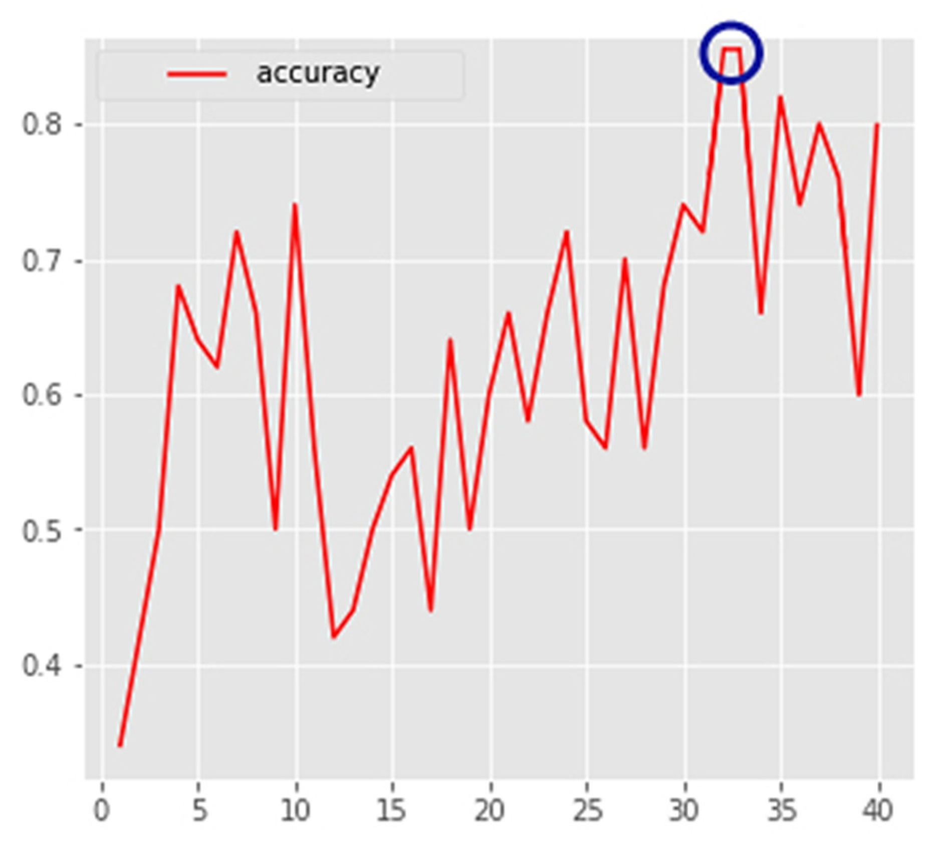
In order to prepare the top three optimum models (Trials 20, 51, and 31) for the Average Ensemble method, we trained them from scratch. Our approach this time was to execute the Keras checkpoint callback at the end of every epoch, thereby saving the weights of the model whenever the validation’s accuracy improved. This allowed us to tune another critical hyperparameter, the number of epochs. Further explanation can be found in Figure 10, where the checkpoint callback saves the weights of the first optimum CNN, at epoch 32. The accuracy of the first, second, and third optimum models increased by 8%, 8%, and 10%, respectively, after applying this method.

The hyperparameters for the first iteration of BO were chosen at random (ReLU activation functions, a dropout rate of 50%, 32 nodes for the first three dense layers, a batch size of 64, and Adam as optimizer) to highlight the benefit of hyperparameter optimization and the usage of checkpoint call back. In

Table 3. Comparison between the performance of the base CNN architecture before and after applying BO and checkpoint callback.

Base CNN Architecture		Accuracy	Precision	Recall	F1-Score	Kappa
Before BO + checkpoint callback		68	58	68	62	54.7
After BO + checkpoint callback	1st optimum CNN	88	90	88	88	84.01
	2nd optimum CNN	88	88	88	88	83.97
	3rd optimum CNN	86	86	84	84	78.63
	Average	87.3	88	86.6	86.6	82.2

, we compare the performance of the base CNN architecture, before and after applying BO and checkpoint call back. It is evident that the performance of our Base CNN model drastically improved after optimizing the activation function, the dropout, the number of nodes, the optimizer, the batch size, and the number of epochs. In terms of the average performance of the three top CNNs, we notice an average increase of 19.3%, 30%, 18.6%, 24.6%, and 27.5% in Accuracy, Precision, Recall, F1-score, and Kappa, respectively.

We combined our three generated CNNs using the Average Ensemble strategy. The performance evaluation metrics for the proposed models are shown in

Table 4. The performance evaluation metrics for the proposed models.

Models	Labels	Precision	Recall	F1-Score	Accuracy	Kappa
1st optimum CNN	Left hand	92	79	85	88	84.01
	Right hand	100	83	91
	Both feet	92	92	92
	Tongue	75	100	86
	Average	90	88	88
2nd optimum CNN	Left hand	93	93	93	88	83.97
	Right hand	75	75	75
	Both feet	92	100	96
	Tongue	91	83	87
	Average	88	88	88
3rd optimum CNN	Left hand	79	79	79	84	78.63
	Right hand	75	100	86
	Both feet	91	83	87
	Tongue	100	75	86
	Average	86	84	84
Average Ensemble	Left hand	100	93	96	92	89.33
	Right hand	79	92	85
	Both feet	100	100	100
	Tongue	91	83	87
	Average	93	92	92

. Precision is described as the positive predictive rate. Based on Precision results, our Ensemble method surpassed the weak-learners’ average Precision by 5.7% which indicates the feasibility and superiority of Ensemble model designed in this paper. Moreover, it provided 100% Precision on the left hand and both feet, stressing the importance of aggregating the performance of multiple weak learners. Our Ensemble method’s Recall exceeded the average Recall of the weak learners by 5.34%. The F1-score reported a similar increase value (5.34%) on the other side. The “feet” label was identified with 100% confidence based on the three aforementioned metrics. In terms of Accuracy score, our Ensemble technique achieved 92%, representing a 5.34% improvement over the weak learners. This is the same increase rate recorded for Recall and F1-score. Cohen’s kappa is an important statistic that measures inter-annotator agreement. The employed Ensemble method scored the highest kappa score, reflecting a 7.13% increase over the weak learners. This significant increase in Precision (5.7%), Recall (5.34%), Accuracy (5.34%), F1-score (5.34%), and Kappa (7.13%) demonstrates the feasibility and superiority of the Ensemble model proposed in this study. Overall, the Ensemble method produces extremely promising results across all five metrics.

Table 5. Comparison with traditional ML algorithms.

Classifiers	Precision	Recall	F1-Score	Accuracy	Kappa
LDA	70.21	68.15	68.2	68	57.22
SVM	70.24	70.83	70.35	70	60.02
RF	59.29	58.15	58.05	58	44.02
MLP	64.81	64.23	63.97	64	52.02
GNB	40.18	40.18	39.45	40	20.13
Average Ensemble of BO-CNNs	93	92	92	92	89.33

compares our optimized Average Ensemble model to five traditional ML algorithms (LDA, SVM, RF, MLP, and GNB) on the BCI Competition IV-2a dataset. All the traditional classifiers were evaluated using the same metrics. Our proposed method outperformed the traditional algorithms by a wide margin across all five metrics. Among the traditional algorithms, SVM classifier performs the best, with a Precision of 70.2%, a Recall of 70.83%, an F1-score of 70.35%, an Accuracy of 70%, and a Kappa score of 60.02%, whereas GNB is the worst classifier in this experiment.

CNN can learn complicated features from a heterogeneous dataset, with the ability to expose the dataset’s hidden characteristics while performing data fitting. Traditional ML algorithms generally build their models from a fixed set of functions, limiting the model’s representation capability.

We evaluated our EL-based model against state-of-the-art methods [19,20,21,22,23,24,25,26] using the same dataset (BCI Competition IV-2a dataset) for fair comparison (

Table 6. Comparison with state-of-the-art methods [19,20,21,22,23,24,25,26].

Methods	Accuracy
Yang’s method [19]	69.27
Cheng’s method [20]	70.5
Abbas’s method [21]	70.7
Sakhavi’s method [22]	74.46
Zhao’s method [23]	75
Liu’s method [24]	76.86
Deng’s method [25]	78.9
ZümrayDokur’s method [26]	79.3
Proposed method	92

). The accuracy of our method reached 92%, outperforming all state-of-the-art methods. Average Ensemble, along with the BO-based hyperparameter optimization, boosted CNN performance.

To the best of our knowledge, this is the first study to employ BO for optimum hyperparameter selection in conjunction with the Average Ensemble approach to this specific EEG MI classification problem. This method was found to be the most effective in this experiment, with a Precision of 93%, a Recall of 92%, an F1-score of 92%, an accuracy of 92%, and a kappa score of 89.33%. In the field of medical diagnostics, these values are considered “very good,” and they can be further enhanced by exploring other EL strategies. CNN function evaluation is both time consuming and expensive. In our case, the expensive function is conducted only in a certain area space because the EI acquisition function aided in swiftly locating the search space. The objective function, represented as a GP model, is used to train the model through objective function evaluation. Analytical tracking was done with the GP model because it creates a posterior distribution over the objective function. The EL technique utilized in this study automated the randomization procedure, enabling the researchers and investigators to analyze numerous databases and collect relevant findings. Instead of being limited to a single classifier, they repeatedly construct several classifiers while randomly altering the inputs. We can achieve a more efficient prediction strategy by merging numerous single classifiers into one.

It is true that all three optimum CNNs employ the same topology (two convolutional layers, two batch norm layers, two max pooling layers, three drop out layers, and four dense layers). Each model, however, has various hyperparameter values (dropout rate, activation function, number of dense nodes, batch size, and optimizer) and each model has its own weaknesses. The idea behind employing an ensemble is that by combining various models that represent multiple hypotheses about the data, we can come up with a better hypothesis that is not in the hypothesis space of the models from which the ensemble is constructed. The three models are complementary in that if one fails, the other succeeds. The accuracy of this Ensemble method was higher than when a single model was used. This demonstrates the efficiency of ensemble learning.

4. Conclusions

MI-BCI applications for rehabilitation require a superior performance level and robustness. The findings of our paper confirm the high potential of our Bayesian optimized ensembled CNN model for real-life applications. However, more advanced results could be reached by examining other EL strategies along with better hyperparameter optimizers.