Predicting Algorithm of Tissue Cell Ratio Based on Deep Learning Using Single-Cell RNA Sequencing

Abstract

Background: Understanding the proportion of cell types in heterogeneous tissue samples is important in bioinformatics. It is a challenge to infer the proportion of tissues using bulk RNA sequencing data in bioinformatics because most traditional algorithms for predicting tissue cell ratios heavily rely on standardized specific cell-type gene expression profiles, and do not consider tissue heterogeneity. The prediction accuracy of algorithms is limited, and robustness is lacking. This means that new approaches are needed urgently. Methods: In this study, we introduced an algorithm that automatically predicts tissue cell ratios named Autoptcr. The algorithm uses the data simulated by single-cell RNA sequencing (ScRNA-Seq) for model training, using convolutional neural networks (CNNs) to extract intrinsic relationships between genes and predict the cell proportions of tissues. Results: We trained the algorithm using simulated bulk samples and made predictions using real bulk PBMC data. Comparing Autoptcr with existing advanced algorithms, the Pearson correlation coefficient between the actual value of Autoptcr and the predicted value was the highest, reaching 0.903. Tested on a bulk sample, the correlation coefficient of Lin was 41% higher than that of CSx. The algorithm can infer tissue cell proportions directly from tissue gene expression data. Conclusions: The Autoptcr algorithm uses simulated ScRNA-Seq data for training to solve the problem of specific cell-type gene expression profiles. It also has high prediction accuracy and strong noise resistance for the tissue cell ratio. This work is expected to provide new research ideas for the prediction of tissue cell proportions.

1. Introduction

Bulk RNA sequencing (RNA-Seq) is used to sequence cell populations whose results reflect the average expression of the overall cell populations. However, cell populations include many different types of cells, and bulk RNA-Seq data can not reveal cellular heterogeneity [1,2]. Therefore, investigating the composition of cell populations is crucial to study the heterogeneity of cells. Inferring the cellular composition of a sample involves determining the existing cell types and corresponding proportions, which is also called cell deconvolution. This reflects many aspects of studying cell heterogeneity. For example, tumor cells have strong cellular heterogeneity and, by assessing the makeup of immune cells in the tumor microenvironment, we can learn the degree of tumor invasion, judge relevant cancer prognostic biomarkers, and analyze the patient’s prognosis and survival condition [3,4,5]. Cell deconvolution can be used to standardize immune profiles in human health and disease, explore pathogenesis, etc. [6,7,8,9,10]. It can also help in the study of cellular heterogeneity during organ development [11,12]. It contributes to determining whether the changes in tissue cell composition are caused by changes in gene expression of specific cell populations or by changes in the composition. Therefore, studying cell deconvolution is essential.

The gene expression value of a heterogeneous sample can be modeled as a linear combination of gene expression values for all cell types in the sample. It is represented by a matrix that the gene expression information of the sample (S) = the gene expression information of each cell type (C) × the ratio of cell types in the sample (R) [13]. The derivation of R through S and C, that is, using a specific express matrix of cell type C, is called a reference-based method, and the method of directly deriving C through S is called a non-reference-based method. A precondition for cell-reference-based deconvolution methods is that the number of equations (number of genes) far exceeds the number of unknowns (total number of cell types in the cell population) [14]. These methods rely heavily on the design of C, and the acquisition of C depends on the marker genes of various cell types, where marker genes are also called signature genes. Therefore, acquiring C can be challenging.

By comparing the gene expression of different cell types, a set of genes are screened as signature genes to distinguish one cell type from others. We generally use “highly expressed, cell-specific” genes. Then, gene values are continually compared for selection and, finally, the top n genes of each cell type are combined to form a signature gene set [15]. Therefore, the design of C is regarded as a screening problem of marker genes. Gini coefficients, Jensen Shannon divergence, or feature selection can also be used for filtering [16,17,18,19]. Cellmapper assumes that marker genes are associated, and starts with one marker gene in the search for marker genes [20]. Machine learning methods, such as support vector regression, can be used to estimate the probability that a gene is a signature gene, such as CIBERSORT and CIBERSORTx [21,22]. CIBERSORT provides 22 immune cell types of C. Both CIBERSORTx and CIBERSORT provide C for some cell types. In the current reference-based cell deconvolution algorithms, the design of C is still the primary consideration.

However, specific cell type expression matrices should vary for tissue specificity; for example, either different tissues or different regions of the tissue should use different cell expression profiles. Even in samples from the same source, batch effects caused by different experimental equipment and time points will introduce data noise [23,24]. However, the above method uses the average value of gene expression. Currently, the use of non-uniform values of C containing more cell types can be used to partially address the above problems [25]. CPM [26] and MusiC [27] have also been proposed to use ScRNA data to generate tissue-specific signature gene matrices. Because some mutant cells and unknown cells have no reference, the design of their feature matrix is very difficult. After designing C, because the number of equations (the number of genes) far exceeds the number of unknowns (the total number of cell types in the cell population), cell deconvolution can be viewed as solving the overdetermined system of equations. The least squares method is commonly used for solving overdetermined equations, such as in DWLS [28], SpatialDWLS [29], and MusiC.

Non-reference-based methods commonly use algorithms involving non-negative matrix factorization [30,31]. Non-negative matrix factorization needs to generate initializations of C and R. However, the matrix factorization problem may obtain multiple global optimal solutions under the non-negative constraints of the base matrix and the proportional matrix [32]. To obtain a proper solution, new constraints must be added, but cell composition ratios are still hard to find.

Therefore, it is desirable to use the gene expression data of the sample as a model input only, and no longer rely on a specific gene expression profile. Deep learning is a good solution. CNNs are widely used in bioinformatics. For example, CNNs have great potential in biological signal processing of one-dimensional data with specific repetitive patterns, such as genome sequences [33], and two-dimensional matrix data, such as the time-frequency matrix of biological signals. The nodes of the model are robust to noise and other deviations. It is difficult but necessary to build a model with high deconvolution performance and robustness to noise and errors using a deep learning approach such as a CNN. Deep learning requires a large amount of labelled data, but labelled information about bulk RNA-Seq is insufficient. Therefore, we use ScRNA-Seq to simulate the generated bulk RNA data and make predictions based on simulated bulk samples and real samples. ScRNA-Seq provides unbiased, reproducible, high-resolution, and high-throughput transcriptional analysis of single cells, reflecting all gene expression levels in single cells [34]. Single-cell metabolomics examines changes in the metabolic status markers of single cells over time, and faces the problem of the lack of a linear relationship between the number of cell matrices and the number of cell products [35]. Single-cell proteomics can distinguish cell types by differential protein information. Its difficulty lies mainly in the trace amount of protein in a single cell [36]. Three studies have analyzed the cellular heterogeneity from the different perspectives of cells. At present, ScRNA-Seq is the most mature discipline.

In this study, a cellular deconvolution scheme named Autoptcr was constructed. Autoptcr is an algorithm that does not depend on a specific expression matrix reference of the cell type. It can infer cell proportions of tissue directly from the tissue’s gene expression data. Autoptcr first applies a CNN to perform cell deconvolution. Autoptcr is trained on simulated ScRNA-Seq data, which solves the difficulty of deep learning training due to the lack of label information of bulk RNA data. It can fully examine the inner relationship between genes and extract the hidden features from ScRNA-Seq data. We compared Autoptcr with other algorithms, and found that it has better deconvolution performance, which means greater accuracy in predicting the proportion of cell types in heterogeneous tissues. The network nodes are robust to data noise and errors. Autoptcr has high prediction accuracy and strong anti-noise ability.

2. Materials and Methods

2.1. Dataset Collection

Little information is available about the labelling of the cellular composition of the cell population in bulk RNA-Seq data. However, deep learning requires a large quantity of tagged bulk RNA-Seq data for training; thus, we use bulk RNA-Seq data simulated by the ScRNA data to train the model. For each simulated bulk RNA-Seq using ScRNA data of human peripheral blood mononuclear cells, we randomly select 500 ScRNA data from the overall data, merge their gene expression matrix as the gene expression matrix of the simulated bulk RNA data, and then record the proportion of each cell type in the simulated tissue as marker information. In this way, if a certain amount of ScRNA data is available, countless bulk RNA-Seq data with labelling information can be generated.

For convenience, we directly use the simulated bulk RNA-Seq data with labels from Kevin (https://figshare.com/s/e59a03885ec4c4d8153f (accessed on 6 April 2022)), which consists of four datasets: data6k, data8k, donorA, and donorC. There are six cell types, namely, Monocytes, Unknown, CD4Tcells, Bcells, NK, and CD8Tcells, of which Unknown represents the unknown cell type, which is used to predict the unknown cell type. The simulated data contain 32,000 tissue samples, each with 32,738 features.

We tested the model on real bulk RNA-Seq data named PBMC2 with noise and bias. This dataset comprises bulk RNA data of peripheral blood mononuclear cells (from 13 individuals). Each sample contains 17,644 features. It was downloaded from GEO (https://www.ncbi.nlm.nih.gov/geo/ (accessed on 6 April 2022)) with accession number GSE107011.

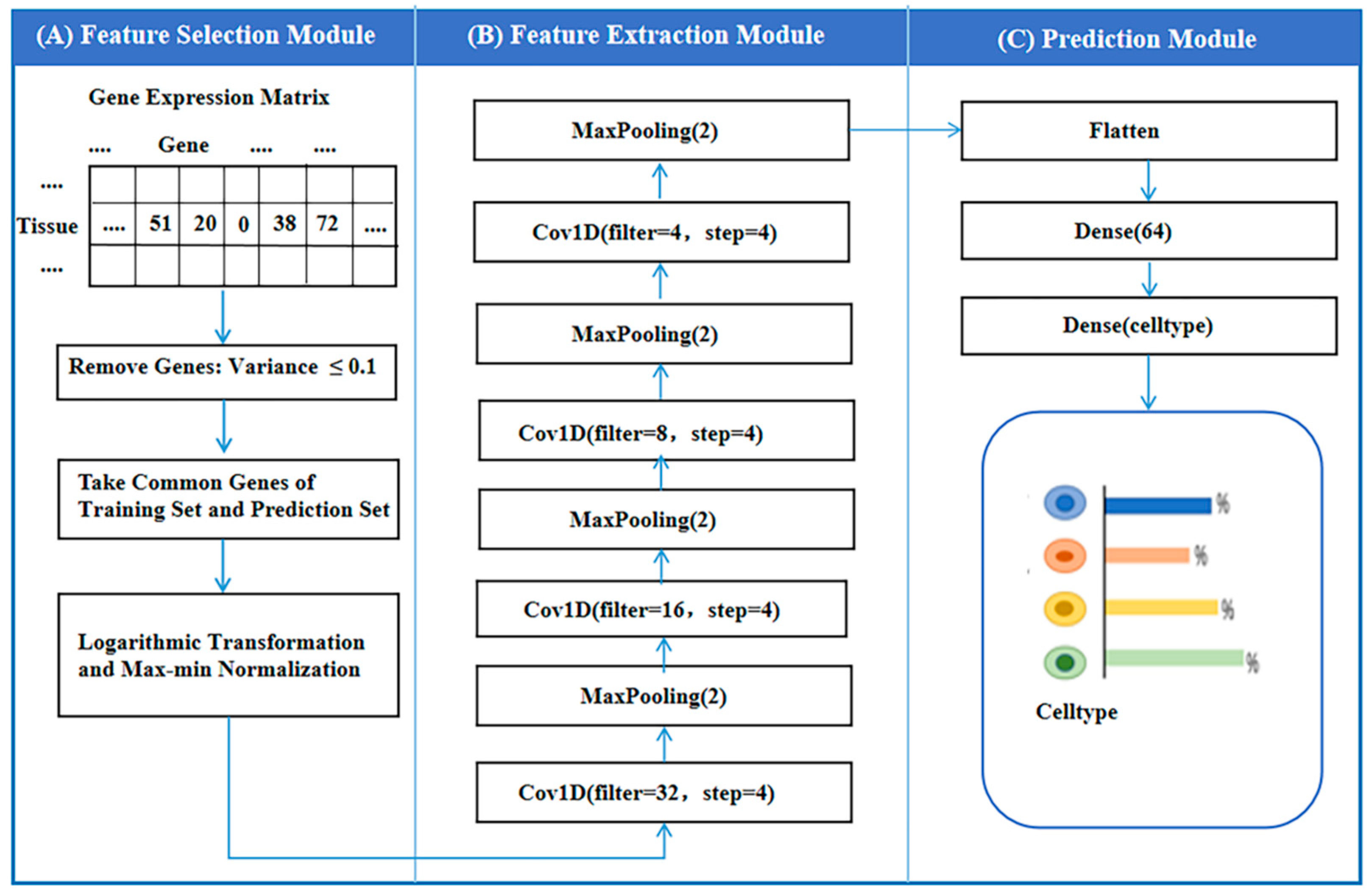
2.2. Structure of Autoptcr Model

In this paper, we propose Autoptcr, a CNN model of a cell deconvolution scheme. As Figure 1 shows, Autoptcr only uses bulk RNA data, namely, the gene expression data of the sample (S), to infer the proportion of cell types in the sample (R). It does not depend on the design of C. The nodes of Autoptcr can learn the relationship between genes in different tissues; that is, the problem that different cell expression profiles should be used for different tissues or different regions of tissues no longer exists. For data noise or bias, nodes in the CNN can learn feature representations that are not affected by bias and noise, and the nodes are robust. There are three modules in our model, namely, a feature selection module, a feature extraction module, and a prediction module.

2.2.1. Feature Selection Module

In the feature selection module, because there are tens of thousands of gene features in the ScRNA-seq data, the simulated Bulk RNA data generated based on it is also the same. Therefore, feature selection is a very important issue. However, we do not perform complex feature selection in this paper; rather, we just remove some unusual features, such as unrelated or underinformed features. Firstly, we perform preprocessing on the gene expression matrix of ScRNA-Seq of simulated tissues, and those features that do not contribute to the results are eliminated. That is, the genes whose expression variance are less than 0.1 are eliminated. Then, we obtain the genes that are in common between the training set and the test set as features. This allows the training and test sets to have the same genes; in this way, we can also make predictions when the features of the training set and the test set are different. This step greatly improves the applicability of the model.

Then, we perform the logarithmic transformation on the gene expression matrix after screening. This step can turn the difference between the data into changes in multiples; as a result, the data is no longer biased in the approximation of the data distribution assumptions for downstream analysis [37], as shown in Equation (1):

$$\tilde{x}={\log }_2(x+1)$$

(1)

where x represents the expression data of a certain gene of the gene expression information of all tissues, and $\tilde{x}$ represents the expression data of a certain gene of the gene expression information of all tissues after transformation.

Then, we perform maximum and minimum normalization on the gene expression matrix [38]. When we train the neural network, the convergence of the weight parameters can be accelerated by standardizing the data. We obtain x’ after preprocessing, as shown in Equation (2):

$$x^{\prime }=\frac{\tilde{x}-\min (\tilde{x})}{\tilde{x}-\max (\tilde{x})}$$

(2)

where x’ represents the expression level data of a certain gene of the gene expression information of all tissues after the maximum and minimum normalization.

2.2.2. Feature Extraction Module

The features filtered by the feature selection module are input into the feature extraction module, and the feature extraction layer uses convolution and pooling techniques. We use $X\in R^{M\times N\times D}$ to represent the input, M is the number of features, N is set to 1, and D represents the number of channels, and is set to 1. The input $X\in R^{M\times 1\times D}$ represents D one-dimensional feature vectors, and the size of the feature is M × 1. The filter is $W\in R^{A\times B\times D\times V}$. A and B represent the length and width of the convolution kernel, and V represents the number of convolution kernels. The convolution kernel is convolved with the two-dimensional vector of the same size on X to obtain the scalar data z, as shown in Equation (3):

$$z={\displaystyle \sum _{a,b}{x}_{a,b}·W_{v,a,b}}$$

(3)

$$a=1,2,\dots ,A;b=1,2,\dots ,B$$

In the above equations, $W_v\in R^{A\times B}$ represents the size of the convolution kernel, and $x\in R^{A\times B}$ represents a 2D vector block on X of the same size as the convolution kernel W_v. To calculate feature the map Y_v, we add kernel $W^{v,\mathbf{1}},W^{v,\mathbf{2}},\dots ,W^{v,D}$ to the feature map $X^1,X^2,\dots ,X^D$, respectively. Then, we add bias to obtain the input of the convolutional layer $Z^v\in R^{M^{\prime }\times N^{\prime }\times \mathbf{1}}$. M’ and V’ depend on the value of padding and stride of the convolutional layer. After the activation function, the final output map Y^v is obtained. In this paper, the value of A is 1 and the value of B is 4. There are four convolutional layers in total, and the number of V is set to 32, 16, 8, and 4, respectively. The filter is $W\in R^{4\times 1\times D\times V}$, as shown in Equations (4) and (5):

$$Z^v={\displaystyle \sum _{d=1}^D{W}^{v,d}\cdot X^d+b^v}$$

(4)

$$Y^v=r(Z^v)$$

(5)

In the above equation, $r(\cdot )$ is the nonlinear activation function. Relu is the most commonly used activation function. We need to output V feature maps, and repeat the above process V times to obtain V feature maps $Y^1,Y^2,\dots ,Y^V$. The activation functions in the convolution kernel are all set to Relu.

The pooling layer downsamples the regions and generalizes them as regions. Suppose the input feature map of the pooling layer is $Z^v\in R^{M^{\prime }\times 1\times \mathbf{1}}$; we then divide $Y^v$ into many regions $O_{e,g}$, $\mathbf{1}\le e\le E$, $\mathbf{1}\le g\le G$. We take E as 1 and G as 2. Regions do not overlap in this paper. $Y_{\stackrel{⌣}{E}}$ is the activity data of neurons in area $O_{e,g}$. For this region, we select the maximum value of all neuron activity in this region, as shown in Equation (6):

$${\stackrel{⌢}{Z}}_{\stackrel{⌣}{E}}=\underset{\stackrel{⌣}{E}\in O_{e,g}}{{\displaystyle \mathrm{Max}}}(Z_{\stackrel{⌣}{E}})$$

(6)

Overall, in Autoptcr, the pooling layer uses max pooling, which reduces the size of the network by reducing the extracted features by more than half. Autoptcr uses one layer of convolution and one layer of max pooling as feature extraction, and the number of V is set to 32, 16, 8, and 4, respectively.

2.2.3. Feature Prediction Module

In the prediction module, for the high-dimensional data extracted by the convolutional network, a flattening function is used to flatten the features to convert the data into one dimension. The one-dimensional data is fed into a fully connected dense layer. Suppose we accept k inputs as $x^1,x^2,\dots ,x^k$; z is used to denote the weighted sum of the input information as the net input, as shown in Equation (7):

$$z={\displaystyle \sum _{k=1}^K{w}_k{x}_k+b}$$

(7)

where w is a k-dimensional weight vector and b is the bias. The net input is then passed through a nonlinear activation function $f(\cdot )$ to obtain the activity value y of the neuron.

The number of neurons in the first dense layer is set to 64, the activation function applied in this paper uses Softmax for the last dense layer in the prediction module, and the Relu function is used for the remainder of the convolutional layers and dense layers. Because the sum of the cell proportions of the tissue must be 1, and the number of cell proportions of all cell types is greater than 0, Softmax is used as the activation function of the final layer. After the output of the last layer, we use the MSE function to calculate the distance between the true value and the predicted value to optimize the network. We use the MSE loss function, as shown in Equation (8):

$$\mathrm{MSE}=\frac{1}{t}{\displaystyle \sum _{i=1}^t({\widehat{Z}}_i-Z_i{)}^2}$$

(8)

where ${\widehat{Z}}_i$ is the predicted cell proportion fraction, Z_i is the actual cell proportion fraction, and t is the number of cell types in the tissue.

2.3. Evaluation Indicators

To verify the model’s performance, we set up evaluation metrics to evaluate the model’s performance. Because we need to predict the proportion of cells of each cell type in the tissue, we cannot judge the model’s accuracy but only judge the quality of the model by the distance between the predicted value and the true value. The evaluation of the performance of Autoptcr uses the root mean square error (RMSE), Pearson correlation coefficient (PCC), and Lin’s consistency correlation coefficient (LCC).

RMSE is used to measure the deviation between variables, as shown in Equation (9):

$$\mathrm{RMSE}\left(z,z^{\prime }\right)=\sqrt{\mathrm{avg}{(z-z^{\prime })}^2}$$

(9)

Pearson’s correlation coefficient (PCC) can measure the degree of correlation between variables, as shown in Equation (10):

$$\text{PCC}\left(z,z^{\prime }\right)=\frac{\text{cov}\left(z,z^{\prime }\right)}{{\partial }_z{\partial }_{z^{\prime }}}$$

(10)

Lin’s consistent correlation coefficient (LCC) can measure both correlation and absolute difference, as shown in Equation (11):

$$\mathrm{LCC}\left(z,z^{\prime }\right)=\frac{2{\partial }_z{\partial }_{z^{\prime }}\times \text{PCC}\left(z,z^{\prime }\right)}{{\partial }_z^2+{\partial }_{z^{\prime }}^2+({\gamma }_z-{\gamma }_{z^{\prime }})}$$

(11)

where z is the actual cell ratio; $z^{\prime }$ is the predicted cell ratio; ${\partial }_z$ and ${\partial }_{z^{\prime }}$, respectively, represent the standard deviations of the predicted and actual cell ratios; and ${\gamma }_z$ and ${\gamma }_{z^{\prime }}$. represent the mean values of the predicted and actual cell ratios, respectively.

2.4. Algorithm of Autoptcr Model

The inputs of data are $\dot{X}$, T, and Z. $\dot{X}=\{{\dot{x}}_1,{\dot{x}}_2,\dots ,{\dot{x}}_q\}$ is a gene set of the trained ScRNA tissues, $\dot{X}$ is a gene in the trained tissues, and q is the number of gene species in the trained tissues. $T=\{t_1,t_2^{},\dots ,t_p\}$ is a gene set of the tested tissues, t is a gene in the tested tissues, and p is the number of gene species in trained tissues. Z is the proportion of cells corresponding to $\dot{X}$. In the screening feature and data transformation work, the data are passed into the convolutional layer and the pooling layer of the feature extraction module, and $r(\cdot )$ is the nonlinear activation function. We set $\mathrm{RELU}(\cdot )$ as the activation function. Then, we enter the predicted cell ratios obtained in the flattened and dense layers of the prediction module. The MSE loss between the real cell proportion and the predicted cell ratios is calculated, using the optimizer OA with a learning rate of LR to optimize the loss function LF of the Autoptcr model. The algorithm description is shown in Algorithm 1.

Algorithm 1 Autoptcr
Begin
1.	Input: $\dot{X}$ is the gene set of the trained ScRNA tissues; Z is the proportion of cells corresponding to $\dot{X}$; T is the gene set of the tested tissues;
2.	Set the hyperparameters of the Autoptcr model, LR = 0.001, OA = Adam, LF = MSE, D = 1, V = 32, S = 2000, BS = 128, $X\leftarrow \varnothing$;
3.	for c = 1 to q do
4.	if feature variance of ${\dot{x}}_c\le 0.1$
5.	$X\leftarrow X\cup \{\varnothing \}$;
6.	else
7.	$X\leftarrow X\cup \left\{{\dot{x}}_c\right\}$;
8.	end for
9.	$X\leftarrow X\cap T$;              //Look for the same genes
10.	Perform a data conversion on X to get X’, X<--X’;
11.	fors = 1 to S do
12.	Sample BS data from X;
13.	For j = 1 to 4 do
14.	for v = 1 to V do            //Determine the number of convolution filters V
15.	$Y^j\leftarrow \mathrm{Relu}({\displaystyle \sum _{d=1}^D{W}_j{}^v\cdot X_j{}^d+b_j{}^v)}$;          //Convolution layer processing
16.	${\stackrel{⌢}{Y}}_{\stackrel{⌣}{E}}{}^j\leftarrow \underset{\stackrel{⌣}{E}\in O_{e,g}}{{\displaystyle \mathrm{Max}}}(Y^j{}_{\stackrel{⌣}{E}})$;          //Maxpooling layer processing
17.	end for
18.	$Y^{j+1}\leftarrow {\stackrel{⌢}{Y}}_{\stackrel{⌣}{E}}{}^j$;
19.	V←V/2;
20.	end for
21.	$X^{\prime }\leftarrow T({\stackrel{⌢}{Y}}_{\breve{E}}{}^j)$, get one-dimensional data;
22.	Input $X^{\prime }$ into two dense layers, get predicted cell ratio of tissue ${\widehat{Z}}_{}$;
23.	Calculate loss function, $\mathrm{MSE}=\frac{1}{t}{\displaystyle \sum _{i=1}^t({\widehat{Z}}_i-Z_i{)}^2}$;
24.	Update the training parameters by OA and LR;
25.	end for
26.	Output: Final predicted cell ratio of tissue Z”;
End

3. Results and Discussion

3.1. Training of Autoptcr

The training set data are input into the Autoptcr network and the network parameters are set. As

Table 1. The hyperparameters of the Autoptcr network.

Parameters	Value
Batch Size	128
Steps	2000
Learning Rate	0.001
Optimized Algorithm	Adam
Loss Function	MSE

shows, this paper uses the MSE function as the loss function. The optimizer is the Adam optimizer. The batch size is 128. The learning rate is 0.001, and 2000 technical steps of early termination are used to prevent the model from overfitting. Regarding the choice of the optimizer, we tested Rmsprop, SGD, etc.; however, the performance of these optimizers is not as good as that of Adam. Regarding overfitting, the performance of the network decreased significantly after using loss regularization. Therefore, we do not set loss regularization in the network and only use the early termination technique to prevent the network from overfitting. After testing, we stop the network after 2000 steps to achieve higher accuracy.

Using simulated bulk RNA data for model training, the data were taken from s different datasets, and X’ was divided into the training set and test set for s-fold cross-validation. The training set consisted of s − 1 pieces of data from different sources and the test set was taken from the remaining one source (500 pieces of data). A total of s experiments were performed. Because the model was trained on the data of different sources, if the model prediction results are excellent, the network nodes of the model can learn features that are robust to errors and noise, and Autoptcr can be used for cell deconvolution. The simulated PBMC data were taken from four datasets: data6k, data8k, donorA, and donorC. We used 4-fold cross-validation, such as training on data6k, data8k, and donorA data, and testing on 500 pieces of donorC data, a total of four times.

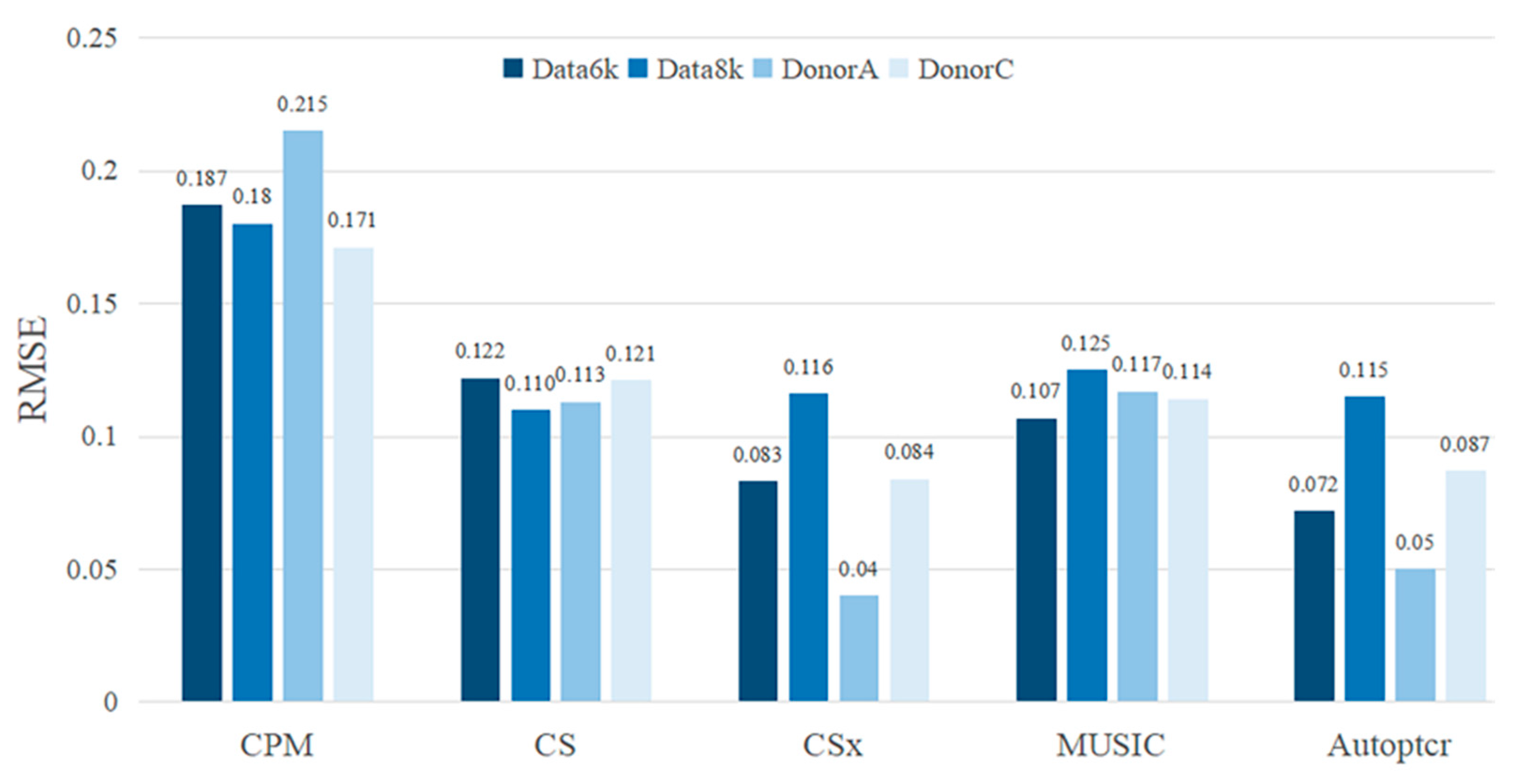
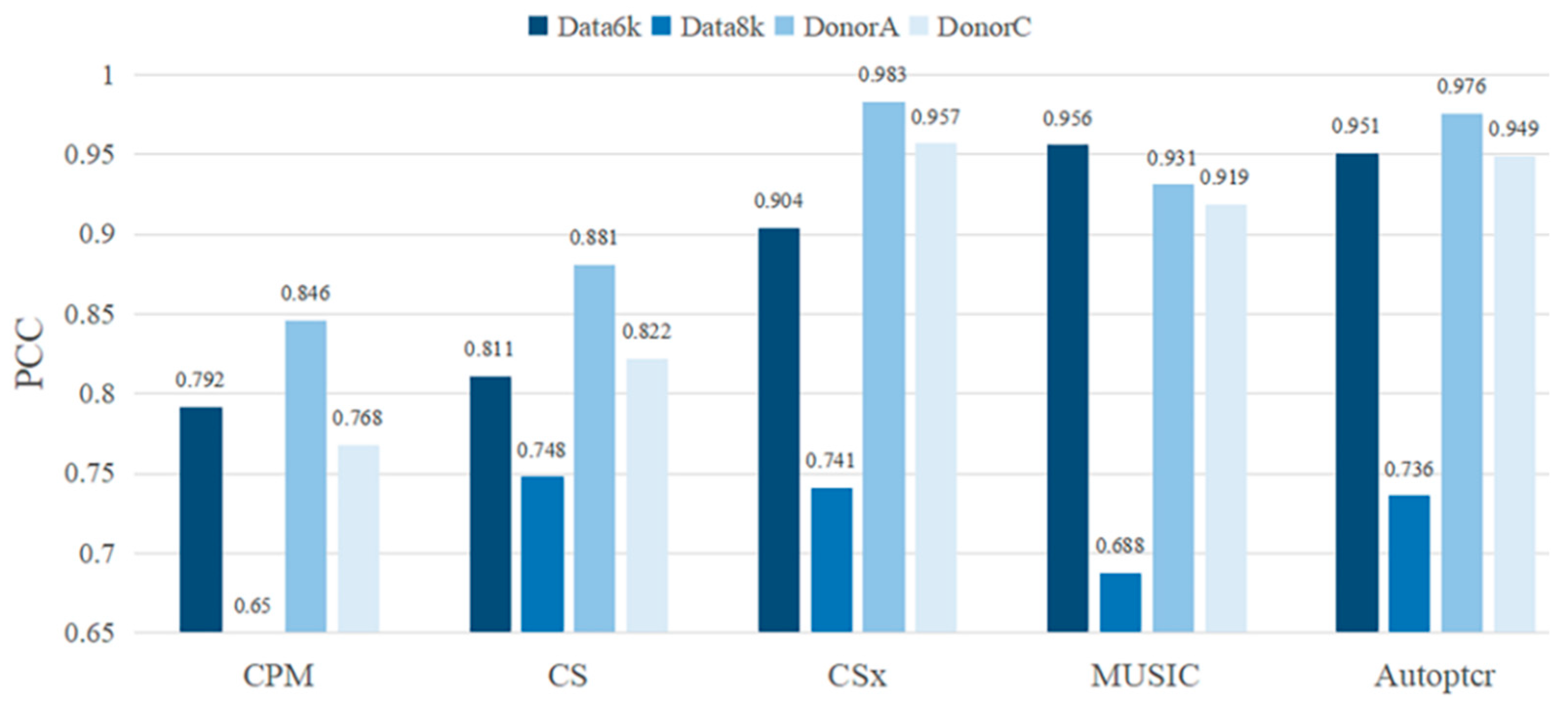
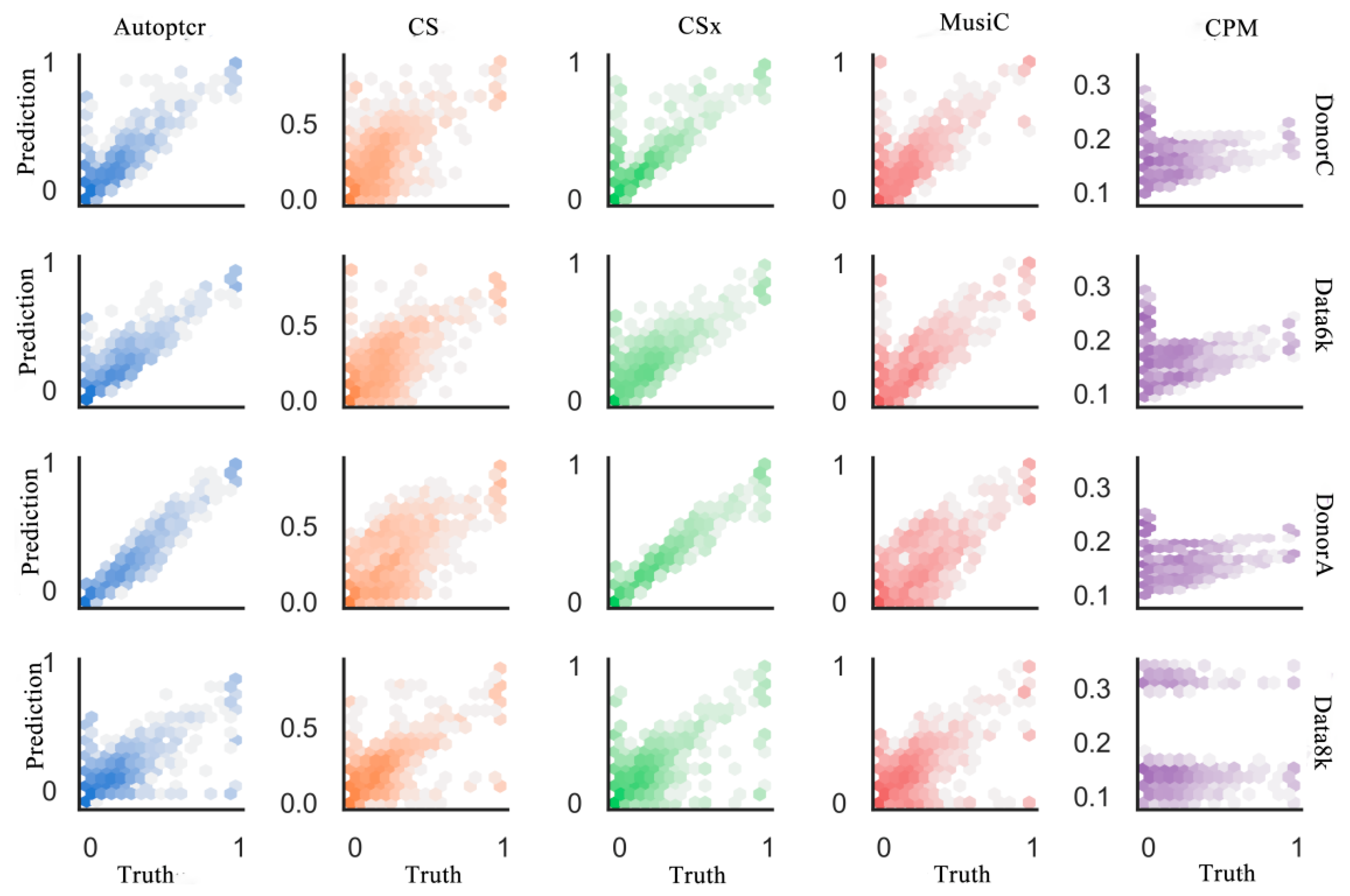
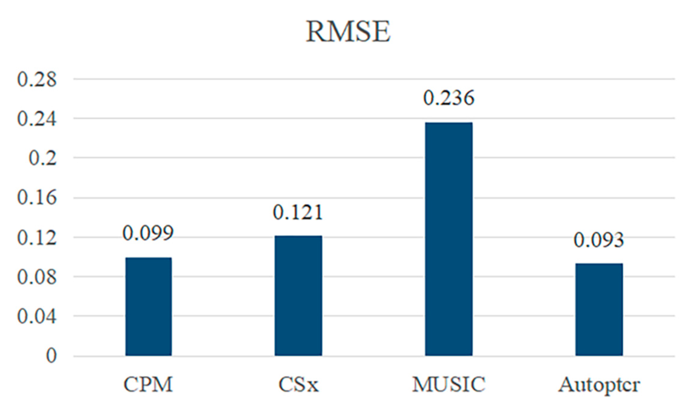
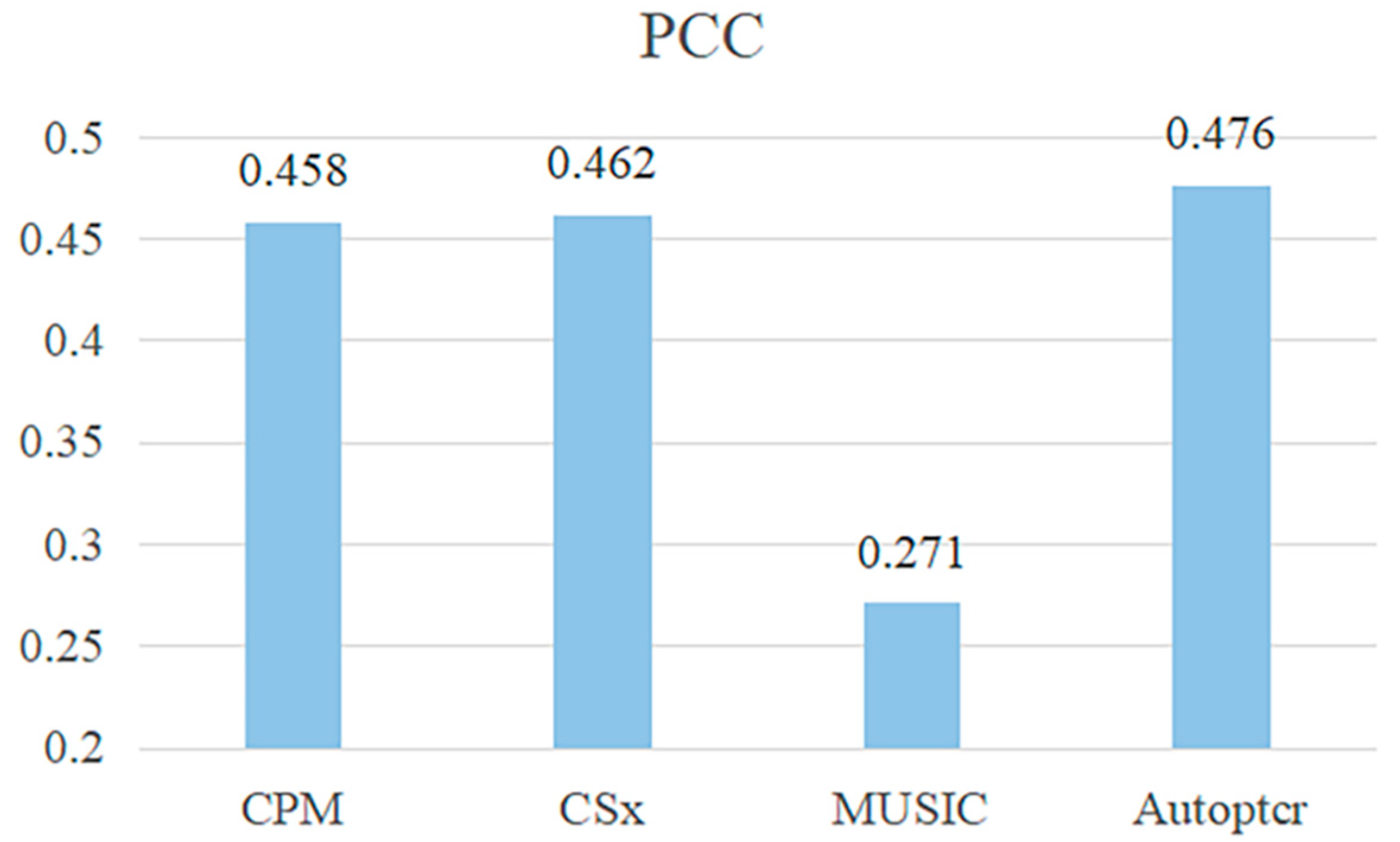
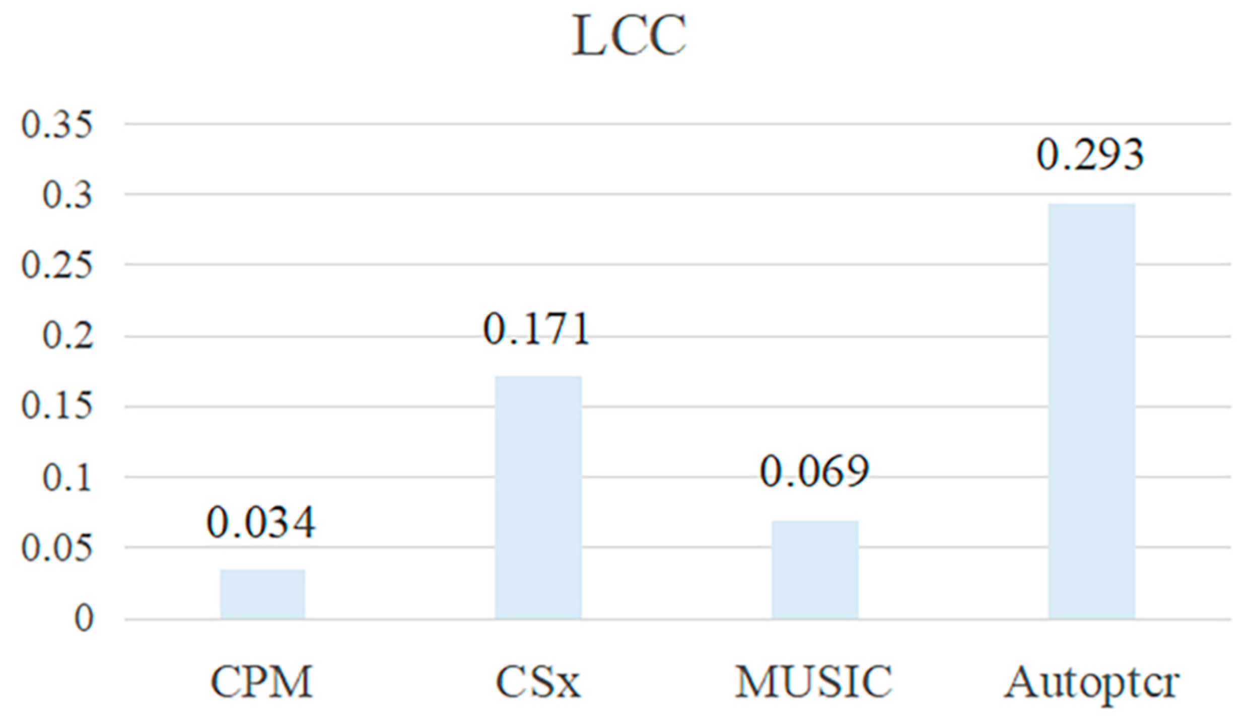
3.2. Test on a Manual Batch Samples

On the trained model, we used the fourth simulated dataset to make predictions to judge the performance of the trained model on the simulated tissue; that is, by determining the error between the predicted value and the actual value. We counted the data and calculated the number of data where the predicted cell ratio differs from the actual cell ratio by 5% and 10%. Among the 500 data used in this paper, 417 data in Bcell met the 5% condition, 332 data in CD4Tcells met the 5% condition, 300 data in CD8Tcells met the 5% condition, 424 data in Monocytes met the 5% condition, 402 data in Unknown were eligible, and 316 data in NK met the 5% condition. A total of 94.3% of the data met the condition of having a difference of less than 10% between the predicted proportion of cells and the actual proportion of cells.

Then, we evaluated the performance of Autoptcr’s prediction using RMSE, PCC, and LCC. The lower the RMSE calculated from the true and predicted values, the closer the values to each other. The higher the PCC and LCC values, the stronger the correlation between the predicted value and the true value. We compared the performance of Autoptcr with that of CIBERSORT (CS), CIBERSORTx (CSx), MusiC, and CPM.

As Figure 2, Figure 3 and Figure 4 show, the comparison of the five methods on different datasets shows that the performance of each method on these datasets is not the same, and there is a certain fluctuation range. Of the four datasets, Autoptcr’s RMSE is at least 0.072 on the data6k dataset, and Autoptcr is the only method having a PCC over 0.94 on the three datasets. Autoptcr’s performance on all four datasets is lower than that of MusiC and CPM in terms of RMSE. CS has the most stable RMSE, and Autoptcr has the smallest dynamic range. The performance of Autoptcr is basically on par with that of CSx.

Finally, we evaluated the average performance of the methods on all datasets. As shown in

Table 2. Average performance of CPM, CS, CSx, MusiC, and Autoptcr on four datasets.

Method Comparison	Value
	RMSE	PCC	LCC
CPM	0.188	0.599	0.073
CS	0.116	0.815	0.702
CSx	0.081	0.896	0.846
MusiC	0.115	0.873	0.799
Autoptcr	0.081	0.903	0.851

, the RMSE of the Autoptcr model is the lowest at 0.081, which is the same as that of CSx. The RMSE values of the remaining three methods are all above 0.11. The PCC of Autoptcr reaches a maximum of 0.903, and the PCC of CSx reaches 0.896, which is higher than that of CPM. This method improves the result by 50%, and is 10% higher than that of CS and 3% higher than that of MusiC. The LCC data of Autoptcr reaches 0.851, which is also the highest. This illustrates that Autoptcr has better deconvolution performance than that of the other methods and can predict unit deconvolution.

Comparing the overall predicted data and the actual data, in Figure 5 the horizontal axis represents the true value and the vertical axis represents the predicted value. A data point falling on the y = x line means that the two attributes are the same. Therefore, the data tend to the line y = x, which represents the higher accuracy of the data prediction. We can see that the CS values occupy the entire plane. From the donorC, data6k, and data8k datasets, the predicted data of Autoptcr tends to the y = x line and is more concentrated, indicating that it is close to predicting the actual value. The minor errors indicate that the data have high stability compared to those of other algorithm models. The biased data are shown in Figure 5.

The predicted value of the CPM method is always lower than the true value in the picture. On the data8k dataset, all methods do not perform very well; that is, this poor performance is not only seen in the Autoptcr model.

The above results show a CNN can be used for cell deconvolution; in addition, the network nodes of the Autoptcr model can learn high-order representations of gene expression data, and these representations are robust to error and noise. Compared with other algorithms, the accuracy of predicting the proportion of cells is high, and cell deconvolution can be effectively performed.

3.3. Test on a Real Dataset PBMC2

We used the bulk RNA-Seq PBMC2 data, which are drawn from PBMCs of different individuals. Because the data are taken from different individuals, the batch effect and individual differences exist. PBMC2 data include noise and bias. Autoptcr was trained on four simulated PBMC datasets and validated on PBMC2. Autoptcr obtained the lowest RMSE value of 0.093 compared to CPM, CSx, and MUSIC, while obtaining the highest PCC value of 0.476 and the highest LCC value of 0.293; this represents an increase of 41% compared to the second-highest, CSx, as shown in the Figure 6, Figure 7 and Figure 8.

The results show we can use the simulated PBMC data for training, then predict the real bulk data from different individual data. The model is not affected by the differences in the data of different individuals. Moreover, the batch effect is caused by experimental operations, and the trained model can generate robust features for noise and bias.

4. Conclusions

Machine learning and deep learning have been widely used in the field of bioinformatics [39]. Autoptcr uses convolutional neural networks, which represent a new solution for cell deconvolution. Autoptcr does not use a reference-based cell deconvolution protocol, and no longer depends on the average expression matrix data of a specific cell type. Therefore, we no longer need to design a complex data preprocessing process to normalize the average expression matrix of a specific cell type.

Autoptcr is highly robust to noise and deviation. It has obvious advantages over ordinary mathematical models for feature extraction and modeling. Its convolutional layers are responsible for extracting the connections between genes. The layer can abstract these implicit connections into features. In addition, Autoptcr can create different signatures based on different data, so it is beneficial for tissue-specific studies. Because of the natural advantages of the network, nodes are good at mining abstract features from noise and deviation data. The experimental results show that Autoptcr can effectively eliminate the noise and deviation caused by the collection process in the experimental data (such as the batch effect). Compared with the traditional deconvolution algorithm that relies on the design of the average expression matrix of a specific cell type and linear regression, Autoptcr has higher prediction accuracy in most cases, and the model is more tolerant of noise and deviation.

Autoptcr also has many outstanding issues. The training of the deep learning model requires a large quantity of data. However, there is little labelling information in bulk RNA-Seq data. Therefore, the model uses artificially simulated data. The simulated data are generated by subsampling the ScRNA-Seq data of the target tissue. Therefore, we speculate that the prediction will be more accurate if some real tissue sample data are added to the artificial simulation data. Determining if Autoptcr can be used for cross-species data will also be one of our future research works.

In conclusion, Autoptcr is robust to noise and bias. The model is easy to understand and extend. As a result of the development of deep learning technology, we can apply attention mechanisms and long short-term memory networks to cellular deconvolution. We expect deep learning techniques to be a popular research topic for cellular deconvolution.

References

1. Jew, B.; Alvarez, M.; Rahmani, E.; Miao, Z.; Ko, A.; Garske, K.M.; Sul, J.H.; Pietiläinen, K.H.; Halperin, E. Accurate estimation of cell composition in bulk expression through robust integration of single-cell information. Nat. Commun. 2020, 11, 1971. [Google Scholar] [CrossRef] [Green Version]
2. Suvà, M.L.; Tirosh, I. Single-cell RNA sequencing in cancer: Lessons learned and emerging challenges. Mol. Cell 2019, 75, 7–12. [Google Scholar] [CrossRef] [PubMed]
3. Chakravarthy, A.; Furness, A.; Joshi, K.; Ghorani, E.; Ford, K.; Ward, M.J.; King, E.V.; Lechner, M.; Marafioti, T.; Quezada, S.A.; et al. Pan-cancer deconvolution of tumour composition using DNA methylation. Nat. Commun. 2018, 9, 3220. [Google Scholar] [CrossRef] [Green Version]
4. Andersson, A.; Larsson, L.; Stenbeck, L.; Salmén, F.; Ehinger, A.; Wu, S.Z.; Al-Eryani, G.; Roden, D.; Swarbrick, A.; Borg, A.; et al. Spatial deconvolution of HER2-positive breast cancer delineates tumor-associated cell type interactions. Nat. Commun. 2021, 12, 6012. [Google Scholar] [CrossRef]
5. Li, B.; Severson, E.; Pignon, J.C.; Zhao, H.; Li, T.; Novak, J.; Jiang, P.; Shen, H.; Aster, J.C.; Rodig, S.; et al. Comprehensive analyses of tumor immunity: Implications for cancer immunotherapy. Genome Biol. 2016, 17, 174. [Google Scholar] [CrossRef] [PubMed] [Green Version]
6. Salas, L.A.; Zhang, Z.; Koestler, D.C.; Butler, R.A.; Hansen, H.M.; Molinaro, A.M.; Wiencke, J.K.; Kelsey, K.T.; Christensen, B.C. Enhanced cell deconvolution of peripheral blood using DNA methylation for high-resolution immune profiling. Nat. Commun. 2022, 13, 761. [Google Scholar] [CrossRef] [PubMed]
7. Sánchez, J.A.; Gil-Martinez, A.L.; Cisterna, A.; García-Ruíz, S.; Gómez-Pascual, A.; Reynolds, R.H.; Nalls, M.; Hardy, J.; Ryten, M.; Botía, J.A. Modeling multifunctionality of genes with secondary gene co-expression networks in human brain provides novel disease insights. Bioinformatics 2021, 37, 2905–2911. [Google Scholar] [CrossRef]
8. Johnson, T.S.; Xiang, S.; Dong, T.; Huang, Z.; Cheng, M.; Wang, T.; Yang, K.; Ni, D.; Huang, K.; Zhang, J. Combinatorial analyses reveal cellular composition changes have different impacts on transcriptomic changes of cell type specific genes in Alzheimer’s Disease. Sci. Rep. 2021, 11, 353. [Google Scholar] [CrossRef] [PubMed]
9. You, C.; Wu, S.; Zheng, S.C.; Zhu, T.; Jing, H.; Flagg, K.; Wang, G.; Jin, L.; Wang, S.; Teschendorff, A.E. A cell-type deconvolution meta-analysis of whole blood EWAS reveals lineage-specific smoking-associated DNA methylation changes. Nat. Commun. 2020, 11, 4779. [Google Scholar] [CrossRef]
10. Arlehamn, C.S.L.; Dhanwani, R.; Pham, J.; Kuan, R.; Frazier, A.; Dutra, J.R.; Phillips, E.; Mallal, S.; Roederer, M.; Marder, K.S.; et al. α-Synuclein-specific T cell reactivity is associated with preclinical and early Parkinson’s disease. Nat. Commun. 2020, 11, 1875. [Google Scholar] [CrossRef] [PubMed] [Green Version]
11. Asp, M.; Giacomello, S.; Larsson, L.; Wu, C.; Fürth, D.; Qian, X.; Wärdell, E.; Custodio, J.; Reimegård, J.; Salmén, F.; et al. A spatiotemporal organ-wide gene expression and cell atlas of the developing human heart. Cell 2019, 179, 1647–1660. [Google Scholar] [CrossRef] [PubMed]
12. Yu, Q.; Kilik, U.; Holloway, E.M.; Tsai, Y.H.; Harmel, C.; Wu, A.; Wu, J.H.; Czerwinski, M.; Childs, C.J.; He, Z.; et al. Charting human development using a multi-endodermal organ atlas and organoid models. Cell 2021, 184, 3281–3298. [Google Scholar] [CrossRef] [PubMed]
13. Yadav, V.K.; De, S. An assessment of computational methods for estimating purity and clonality using genomic data derived from heterogeneous tumor tissue samples. Brief. Bioinform. 2015, 16, 232–241. [Google Scholar] [CrossRef] [Green Version]
14. Cobos, F.A.; Vandesompele, J.; Mestdagh, P.; Preter, K.D. Computational deconvolution of transcriptomics data from mixed cell populations. Bioinformatics 2018, 34, 1969–1979. [Google Scholar] [CrossRef] [Green Version]
15. Chen, Z.; Ji, C.; Shen, Q.; Liu, W.; Qin, F.X.; Wu, A. Tissue-specific deconvolution of immune cell composition by integrating bulk and single-cell transcriptomes. Bioinformatics 2020, 36, 819–827. [Google Scholar] [CrossRef]
16. Zhang, J.D.; Hatje, K.; Sturm, G.; Broger, C.; Ebeling, M.; Burtin, M.; Terzi, F.; Pomposiello, S.I.; Badi, L. Detect tissue heterogeneity in gene expression data with BioQC. BMC Genom. 2017, 18, 277. [Google Scholar] [CrossRef]
17. Cabili, M.N.; Trapnell, C.; Goff, L.; Koziol, M.; Tazon-Vega, B.; Regev, A.; Rinn, J.L. Integrative annotation of human large intergenic noncoding RNAs reveals global properties and specific subclasses. Genes Dev. 2011, 25, 1915–1927. [Google Scholar] [CrossRef] [Green Version]
18. Becht, E.; Giraldo, N.A.; Lacroix, L.; Buttard, B.; Elarouci, N.; Petitprez, F.; Selves, J.; Laurent-Puig, P.; Sautès-Fridman, C.; Fridman, W.H.; et al. Estimating the population abundance of tissue-infiltrating immune and stromal cell populations using gene expression. Genome Biol. 2016, 17, 218. [Google Scholar] [CrossRef]
19. Wang, N.; Hoffman, E.P.; Chen, L.; Chen, L.; Zhang, Z.; Liu, C.; Yu, G.; Herrington, D.M.; Clarke, R.; Wang, Y. Mathematical modelling of transcriptional heterogeneity identifies novel markers and subpopulations in complex tissues. Sci. Rep. 2016, 6, 18909. [Google Scholar] [CrossRef] [PubMed] [Green Version]
20. Nelms, B.D.; Waldron, L.; Barrera, L.A.; Weflen, A.W.; Goettel, J.A.; Guo, G.; Montgomery, R.K.; Neutra, M.R.; Breault, D.T.; Snapper, S.B.; et al. CellMapper: Rapid and accurate inference of gene expression in difficult-to-isolate cell types. Genome Biol. 2016, 17, 201. [Google Scholar] [CrossRef] [Green Version]
21. Newman, A.M.; Liu, C.L.; Green, M.R.; Gentles, A.J.; Feng, W.; Xu, Y.; Hoang, C.D.; Diehn, M.; Alizadeh, A.A. Robust enumeration of cell subsets from tissue expression profiles. Nat. Methods 2015, 12, 453–457. [Google Scholar] [CrossRef] [PubMed] [Green Version]
22. Newman, A.M.; Steen, C.B.; Liu, C.L.; Gentles, A.; Chaudhuri, A.A.; Scherer, F.; Khodadoust, M.S.; Esfahani, M.S.; Luca, B.A.; Steiner, D.; et al. Determining cell type abundance and expression from bulk tissues with digital cytometry. Nat. Biotechnol. 2019, 37, 773–782. [Google Scholar] [CrossRef]
23. Ziegenhain, C.; Vieth, B.; Parekh, S.; Reinius, B.; Guillaumet-Adkins, A.; Smets, M.; Leonhardt, H.; Heyn, H.; Hellmann, I.; Enard, W. Comparative Analysis of Single-Cell RNA Sequencing Methods. Mol. Cell 2017, 65, 631–643.e4. [Google Scholar] [CrossRef] [PubMed] [Green Version]
24. Svensson, V.; Natarajan, K.N.; Ly, L.H.; Miragaia, R.J.; Labalette, C.; Macaulay, I.C.; Cvejic, A.; Teichmann, S.A. Power analysis of single-cell RNA-sequencing experiments. Nat. Methods 2017, 14, 381–387. [Google Scholar] [CrossRef] [Green Version]
25. Vallania, F.; Tam, A.; Lofgren, S.; Schaffert, S.; Azad, T.D.; Bongen, E.; Haynes, W.; Alsup, M.; Alonso, M.; Davis, M.; et al. Leveraging heterogeneity across multiple datasets increases cell-mixture deconvolution accuracy and reduces biological and technical biases. Nat. Commun. 2018, 9, 4735. [Google Scholar] [CrossRef] [Green Version]
26. Frishberg, A.; Peshes-Yaloz, N.; Cohn, O.; Rosentul, D.; Steuerman, Y.; Valadarsky, L.; Yankovitz, G.; Mandelboim, M.; Iraqi, F.A.; Amit, I.; et al. Cell composition analysis of bulk genomics using single-cell data. Nat. Methods 2019, 16, 327–332. [Google Scholar] [CrossRef]
27. Wang, X.; Park, J.; Susztak, K.; Zhang, N.R.; Li, M. Bulk tissue cell type deconvolution with multi-subject single-cell expression reference. Nat. Commun. 2019, 10, 380. [Google Scholar] [CrossRef] [Green Version]
28. Tsoucas, D.; Dong, R.; Chen, H.; Zhu, Q.; Guo, G.; Yuan, G.C. Accurate estimation of cell-type composition from gene expression data. Nat. Commun. 2019, 10, 2975. [Google Scholar] [CrossRef] [PubMed]
29. Dong, R.; Yuan, G.C. SpatialDWLS: Accurate deconvolution of spatial transcriptomic data. Genome Biol. 2021, 22, 145. [Google Scholar] [CrossRef]
30. Stein-O’Brien, G.L.; Clark, B.S.; Sherman, T.; Zibetti, C.; Hu, Q.; Sealfon, R.; Liu, S.; Qian, J.; Colantuoni, C.; Blackshaw, S.; et al. Decomposing Cell Identity for Transfer Learning across Cellular Measurements, Platforms, Tissues, and Species. Cell Syst. 2021, 12, 203. [Google Scholar] [CrossRef] [PubMed]
31. Tang, D.; Park, S.; Zhao, H. NITUMID: Nonnegative matrix factorization-based Immune-TUmor MIcroenvironment Deconvolution. Bioinformatics 2020, 36, 1344–1350. [Google Scholar] [CrossRef]
32. Kriebel, A.R.; Welch, J.D. UINMF performs mosaic integration of single-cell multi-omic datasets using nonnegative matrix factorization. Nat. Commun. 2022, 13, 780. [Google Scholar] [CrossRef] [PubMed]
33. Zhang, Z.; Park, C.Y.; Theesfeld, C.L.; Troyanskaya, O.G. An automated framework for efficiently designing deep convolutional neural networks in genomics. Nat. Mach. Intell. 2021, 3, 392–400. [Google Scholar] [CrossRef]
34. Kharchenko, P.V. The triumphs and limitations of computational methods for scRNA-seq. Nat. Methods 2021, 18, 723–732. [Google Scholar] [CrossRef] [PubMed]
35. Guo, S.; Zhang, C.; Le, A. The limitless applications of single-cell metabolomics. Curr. Opin. Biotechnol. 2021, 71, 115–122. [Google Scholar] [CrossRef]
36. Doerr, A. Single-cell proteomics. Nat. Methods 2019, 16, 20. [Google Scholar] [CrossRef]
37. Choudhary, S.; Satija, R. Comparison and evaluation of statistical error models for scRNA-seq. Genome Biol. 2022, 23, 27. [Google Scholar] [CrossRef] [PubMed]
38. Vallejos, C.A.; Risso, D.; Scialdone, A.; Dudoit, S.; Marioni, J.C. Normalizing single-cell RNA sequencing data: Challenges and opportunities. Nat. Methods 2017, 14, 565–571. [Google Scholar] [CrossRef]
39. Liu, Z.; Yang, Y.; Li, D.; Lv, X.; Chen, X.; Dai, Q. Prediction of the RNA Tertiary Structure Based on a Random Sampling Strategy and Parallel Mechanism. Front. Genet. 2022, 12, 813604. [Google Scholar] [CrossRef] [PubMed]
Figure 1. The structure of Autoptcr. (A) The feature selection module can screen the genes and transform data. (B) The feature extraction module extracts gene expression intrinsic information using convolution and pooling. (C) The prediction module predicts the cell ratio of the tissue.
Applsci 12 05790 g001
Figure 2. RMSE of CPM, CS, CSx, MusiC, and Autoptcr on four datasets.
Applsci 12 05790 g002
Figure 3. PCC of CPM, CS, CSx, MusiC, and Autoptcr on four datasets.
Applsci 12 05790 g003
Figure 4. LCC of CPM, CS, CSx, MusiC, and Autoptcr on four datasets.
Applsci 12 05790 g004
Figure 5. Comparison of actual and predicted values of Autoptcr, CS, CSx, MusiC and CPM.
Applsci 12 05790 g005
Figure 6. RMSE of CPM, CSx, MusiC, and Autoptcr on PBMC2.
Applsci 12 05790 g006
Figure 7. PCC of CPM, CSx, MusiC, and Autoptcr on PBMC2.
Applsci 12 05790 g007
Figure 8. LCC of CPM, CSx, MusiC, and Autoptcr on PBMC2.
Applsci 12 05790 g008