One-Dimensional Detection Using Interference Estimation by Multilayered Two-Dimensional General Partial Response Targets for Bit-Patterned Media Recording Systems

Abstract

In bit-patterned media recording (BPMR) systems, two-dimensional (2D) interference, which includes intersymbol and intertrack interference from down- and across-track directions, respectively, increases when the distance between the islands is reduced with increasing areal density. In recent studies, a general partial response (GPR) target was often deployed with the equalizer to estimate and reduce interference. With this combination, the BPMR system becomes a promising candidate for high-density storage systems and achieves high bit error rate (BER) performance. Therefore, in this study, we investigate the detection capability while varying the form of the GPR target and implement a multilayered 2D GPR target and a detection method for improving the accuracy in estimating the interference. The simulation results demonstrate that the proposed model improves by a gain of ~1 dB compared to the previous studies.

1. Introduction

With special priority, magnetic recording and semiconductor memory are two types of storage technologies of interest to researchers. In magnetic recording, the magnetized grains contain the data bits [1], whereas, in semiconductor memory, the electrons represent the data bits and are stored in floating gates [2]. The choice between magnetic recording and semiconductor memory depends on a trade-off between data access and price per bit [3]. With the promised capacity, this study focuses on magnetic storage.

In hard-disk drives, the data are stored in a thin magnetic film. One bit of data resides in 20–30 magnetized grains. The energy barrier for thermal switching is proportional to the grain volume, and reducing the grain volume to increase the storage density would result in spontaneous data loss owing to superparamagnetism. Therefore, such drives are limited to an areal density (AD) of ~1 Tb/in² [4]. To overcome this limitation in bit-patterned media recording (BPMR), a thin magnetic film is deposited to enable strong exchange coupling between the grains. The film was patterned into magnetic islands using nanolithography. Moreover, when BPMR is combined with a heat-assisted magnetic recording (HAMR), areal densities of up to 20–300 Tb/in² are predicted [5]. In addition, HAMR [6] and two-dimensional (2D) magnetic recording (TDMR) [3] are new technologies proposed to combat superparamagnetism and improve magnetic storage systems to ultrahigh density.

Among the above technologies, BPMR is a potential future hard-disk drive technology. However, when AD is increased by reducing the distance between magnetic islands, the intersymbol interference (ISI) and intertrack interference (ITI) also increase in the down- and across-track directions, respectively. This is referred to as 2D interference in BPMR systems. In addition, the bit error rate (BER) performance of BPMR is reduced by media noise and track misregistration (TMR) [7,8]. Currently, the AD value of BPMR has been developed up to 4 Tb/in² [8,9].

To overcome these obstacles, signal-processing research has focused on two common approaches: symbol detection and error-control coding and/or modulation coding. In addition, there are collaborating methods in which the feedback line between the detection and error-control and/or modulation coding is designed to create an iterative algorithm.

We used two approaches for modulation coding. First, the symbols must avoid patterns causing errors frequently, for instance, a bit encircled by opposite polarity bits. Second, if the minimum distance between codewords is >1, these symbols can achieve some error-correction capability. Kovintavewat et al. [10] designed an 8/9 2D modulation code to eliminate the fatal interference patterns. With improvement, Nguyen and Lee [11] proposed a rate 9/12 2D modulation code that ensures a reasonable Hamming distance in the codeword set and avoids fatal interference as much as possible. By proposing a 3/4 2D modulation code that removes the ITI. Buajong and Warisarn [12] reduced the ITI in BPMR systems using an array reader. To adapt to the staggered structure of BPMR, Nguyen and Lee [13] designed an error-correcting 5/6 modulation code that can correct the errors and reduce the isolated bit. In addition, Jeong and Lee [14] proposed a multilayer perceptron decoding modulation code for BPMR systems.

To mitigate 2D interference, we used an equalizer and partial-response maximum-likelihood detection. Nabavi and Kumar [15] used a 2D equalizer combined with a general partial response (GPR) target to convert 2D interference into one-dimensional (1D) interference and applied 1D detection. The GPR target is presented as a matrix G, as shown in Figure 1. To avoid using 2D Viterbi detection, Nabavi et al. [16] proposed a modified Viterbi algorithm (MVA) that supplies ITI information for the Viterbi algorithm (VA). Wang and Kumar [17] proposed a hybrid 2D equalizer that was used to improve the MVA when the ITI type was known. Sadeghian and Barry [18] proposed an effective detection technique to combat ITI at a low implementation cost. With the superiority of the soft-output Viterbi algorithm (SOVA), Kim and Lee [19] designed a 2D SOVA that exploits two 1D SOVAs in the horizontal and vertical directions. The original version of the 2D SOVA was introduced to handle the 2D interference in holographic data storage systems; it was later developed into an iterative 2D SOVA for BPMR [20]. However, in these studies, only the 1D form of the GPR target was used (or a 2-way GPR target according to the definition in [21], which is presented in Figure 1). Nguyen and Lee [21] designed feedback for the MVA to apply the 3-way GPR. This model achieves better BER performance than the 2-way GPR target. Finally, based on the decomposition matrix of the GPR target, Nguyen and Lee [22,23] proposed a serial detection method. The GPR target form is very similar to the 8-way GPR target. However, the parameters at the four corners were calculated by multiplying the horizontal and vertical parameters. Therefore, the GPR target in [22,23] is still not a real 8-way GPR target.

In addition to the VA, we can use the Bahl–Cocke–Jelinek–Raviv (BCJR) algorithm for detection in the BPMR system [24,25]. In general, although the BCJR algorithm achieves high performance, its complexity is very high. Therefore, when researchers design detection schemes, they mostly focus on the VA.

In this study, we analyzed various types of N-way GPR combined with detection. Based on the complexity problem of 2D Viterbi detection, we propose a 1D Viterbi detection scheme for an 8-way GPR target. In the detection of this GPR target, ITI information is supplied to convert the 2D detection into 1D detection with the same performance and reduced complexity. The proposed scheme extracts the ITI information supplied from multiple GPR targets instead of exploiting multi-head multitrack to subtract the ITI, as in [12,26,27,28,29]. The proposed model exploits multiple layers of GPR targets to estimate each layer of original data. In each layer, the accuracy of the estimated data gradually improved. Therefore, this model is close to the ideal case. The results demonstrate that our model improves the BER performance of the BPMR systems. Generally, detection is based on a GPR target. Therefore, well-designed GPR targets must fit the interference forms, and the final detection that removes the interference can improve the accuracy. The contributions of this study are as follows:

• We propose an interference estimation method and design a simple 1D detection scheme for the 8-way GPR target instead of the 2- or 4-way GPR targets in the previous works.
• We analyzed the latency and suggested a method to reduce it.
• We compared the complexity of the proposed method with that of previous methods.

The remainder of this paper is organized as follows. In Section 2, we analyze N-way GPR with detection and interpret N-way detection. Based on Section 2, we propose a detection scheme for an 8-way GPR target in Section 3. The simulation results and discussion are presented in Section 4. Section 5 presents the complexity and latency issues of the proposed method compared with those of previous methods. Finally, conclusions are presented in Section 6.

2. N-Way GPR Target and Detection

In this section, we explain N-way GPR targets and detection. In addition, we show the complexity of detection depending on the form of the N-way GPR target.

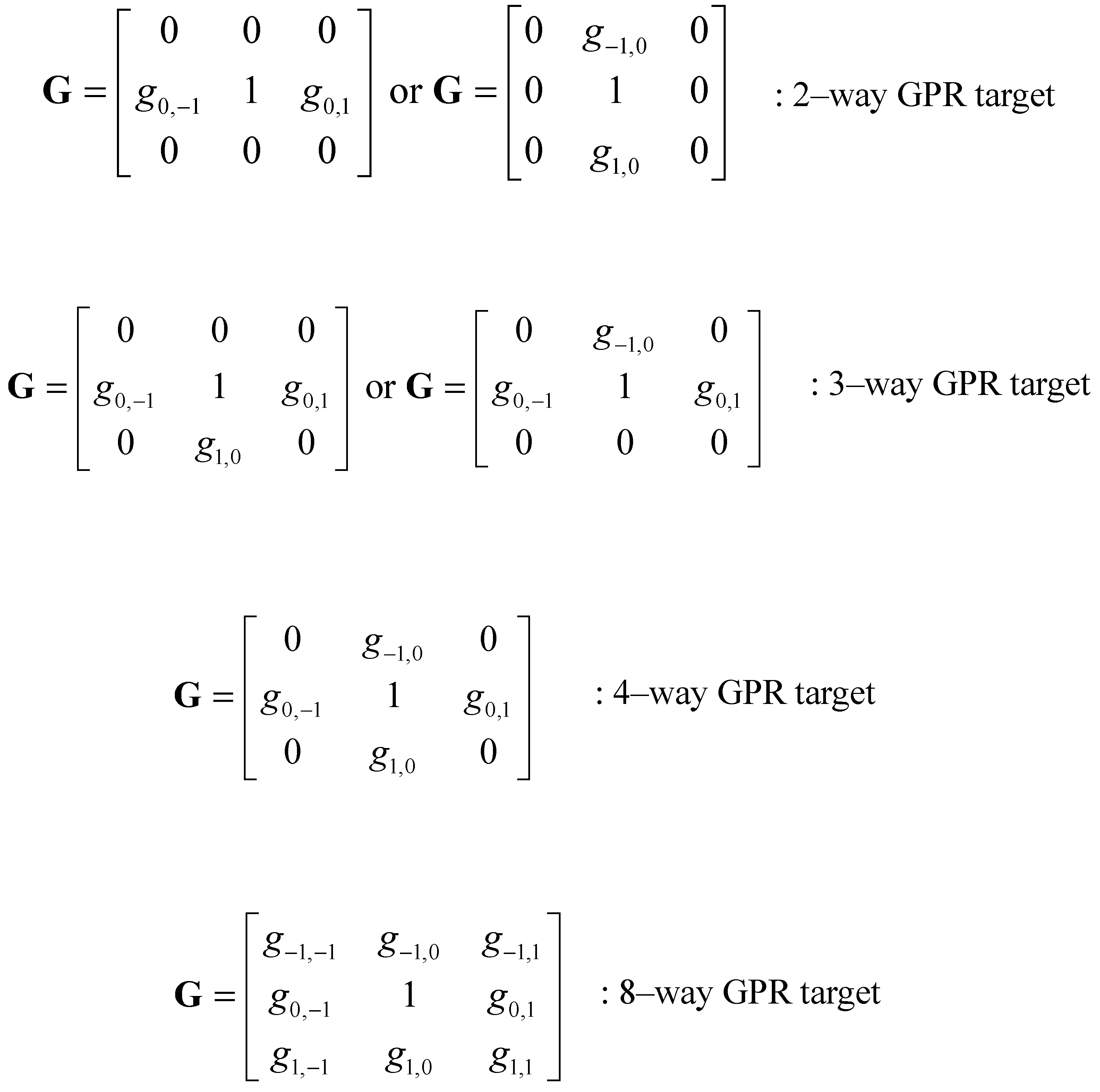
2.1. GPR Target and Equalizer

In Figure 2, we use the training data to collect signals a[j,k] and y[j,k] during the training process. We use equalizer F to match GPR target G, which is determined by the minimum mean square error (MMSE) algorithm during the training period. To implement the GPR target and equalizer, we require a buffer to process each data page [15]. We estimated parameters F and G in the training process. The forms of the matrices F and G are as follows:

$$F=\left[\begin{array}{ccccc}{f}_{-2,-2}& f_{-2,-1}& f_{-2,0}& f_{-2,1}& f_{-2,2}\\ f_{-1,-2}& f_{-1,-1}& f_{-1,0}& f_{-1,1}& f_{-1,2}\\ f_{0,-2}& f_{0,-1}& f_{0,0}& f_{0,1}& f_{0,2}\\ f_{1,-2}& f_{1,-1}& f_{1,0}& f_{1,1}& f_{1,2}\\ f_{2,-2}& f_{2,-1}& f_{2,0}& f_{2,1}& f_{2,2}\end{array}\right],$$

(1)

$$G=\left[\begin{array}{ccc}{g}_{-1,-1}& g_{-1,0}& g_{-1,1}\\ g_{0,-1}& g_{0,0}& g_{0,1}\\ g_{1,-1}& g_{1,0}& g_{1,1}\end{array}\right],$$

(2)

From the definitions and equations in the Appendix A, we can obtain each type of GPR target, as shown in Figure 1.

2.2. Detection

Based on the N-way GPR targets identified, we designed the detection for each N-way GPR target. First, with the 2-way GPR target, we used the conventional VA to implement detection. The trellis, in this case, includes four states and two branches in each state, as shown in Figure 3. Next, we considered a 3-way GPR target. The trellis includes eight states and four branches in each state (Figure 4). However, we can use the MVA with feedback in [21] to reduce the complexity of detection for a 3-way GPR target. Simultaneously, the detection performance of [21] was better than that of the trellis, as shown in Figure 4.

Next, we considered a 4-way GPR target. The trellis includes 16 states and eight branches in each state. Because this trellis has high complexity, Nguyen and Lee [21] also proposed the detection of a 4-way GPR target.

Finally, the detection trellis for the 8-way GPR target exhibited the highest complexity. The trellis includes 64 states and eight branches in each state. Nguyen and Lee [22,23] designed serial detection (Figure 5) for when the GPR target is closer to the 8-way GPR. This is an approximation of the true 8-way GPR and can be decomposed as follows:

$$G=\left[\begin{array}{ccc}rp& p& rp\\ r& 1& r\\ rp& p& rp\end{array}\right]=\left[\begin{array}{ccc}0& p& 0\\ 0& 1& 0\\ 0& p& 0\end{array}\right]\left[\begin{array}{ccc}0& 0& 0\\ r& 1& r\\ 0& 0& 0\end{array}\right].$$

(3)

The trellis of the horizontal detector includes 36 states and six branches in each state, and the trellis of the vertical detector has four states and two input/output branches in each state.

The true 8-way GPR target has the following form:

$$G=\left[\begin{array}{ccc}t& p& t\\ r& 1& r\\ t& p& t\end{array}\right],$$

(4)

where the parameter t must be independent of the parameters p and r. This fact was not addressed in [22,23] and is resolved in Section 3.

We also calculated the MMSE of each GPR target. The results are listed in

Table 1. MMSE results according to the signal-to-noise ratio (SNR).

	SNR (dB)	10	11	12	13	14	15
GPR
2-way		0.0955	0.0784	0.0638	0.0522	0.0424	0.0344
3-way		0.0962	0.082	0.0726	0.0614	0.0577	0.0504
4-way		0.0858	0.0702	0.0571	0.0465	0.0377	0.0305
$\tilde{\mathbf{8}}$-way (3)		0.0793	0.0651	0.053	0.0434	0.0353	0.0287
8-way (4)		0.0707	0.0577	0.0467	0.038	0.03	0.0248

. Here, we can see that the performance improved as the value of N increased (the best results are bold). Except for the 3-way GPR target, because the channel is affected by asymmetric interference, when applying the 3-way GPR target, these interferences will be deflected in one direction, and the equalizer cannot estimate the signal to achieve better MMSE compared to that of the 2-way GPR target. The $\tilde{8}$-way GPR target (Equation (3)) and 8-way GPR target (Equation (4)) appear to achieve similar performance. However, the 8-way GPR target was the most accurate. Therefore, although designing the detection for the 8-way GPR target is very difficult, building a suitable detection method for the 8-way GPR target is still needed.

Next, we calculated the complexity of detection for each GPR target. Here, we only considered the raw VA with a trellis, as shown in Figure 3 and Figure 4, ignoring the modified models for the VA.

Table 2. Complexity of detection for each GPR target.

	Operator	Multiplication and Division	Addition and Subtraction
GPR
2-way		8	24
3-way		32	96
4-way		128	384
$\tilde{\mathbf{8}}$-way		224	672
8-way		512	1536

lists the number of operations per bit of detection for each GPR target.

From Table 2, we see that the detection for the 8-way GPR is highly complex. Therefore, researchers avoided using the raw VA model in this case. Instead, they always attempted to modify the VA to match the 8-way GPR target, as in [22,23]. In the next section, we propose models that improve the performance and reduce the complexity of an 8-way GPR target.

3. Proposed Model

3.1. Detection for an 8-Way GPR Target

In Figure 6, the output of equalizer z[j,k] is presented as follows:

$$z\left[j,k\right]=d\left[j,k\right]+w_{\mathbf{F}}\left[j,k\right]={\displaystyle \sum _{n=-1}^1{\displaystyle \sum _{m=-1}^{1}a\left[j-n,k-m\right]g_{n,m}}}+w_{\mathbf{F}}\left[j,k\right],$$

(5)

where w_F[j,k] is the color noise, which is minimized in the MMSE algorithm. Therefore, we ignore w_F[j,k] when analyzing the estimated signal to design detection.

In this section, we use the 8-way GPR target. Therefore, matrix G has the form

$$G=\left[\begin{array}{ccc}t& p& t\\ r& 1& r\\ t& p& t\end{array}\right].$$

We can expand (5) as follows:

$$g_1^T{a}_{k-1}+g_0^T{a}_k+g_{-1}^T{a}_{k+1}={\displaystyle \sum _{i=-1}^1{g}_i^T{a}_{k-i}},$$

(6)

where

$$g_{-1}={\left[\begin{array}{ccc}t& r& t\end{array}\right]}^T,$$

(7)

$$g_0={\left[\begin{array}{ccc}p& 1& p\end{array}\right]}^T,$$

(8)

$$g_1={\left[\begin{array}{ccc}t& r& t\end{array}\right]}^T,$$

(9)

$$a_{k-1}={\left[\begin{array}{ccc}a\left[j-1,k-1\right]& a\left[j,k-1\right]& a\left[j+1,k-1\right]\end{array}\right]}^T,$$

(10)

$$a_k={\left[\begin{array}{ccc}a\left[j-1,k\right]& a\left[j,k\right]& a\left[j+1,k\right]\end{array}\right]}^T,$$

(11)

$$a_{k+1}={\left[\begin{array}{ccc}a\left[j-1,k+1\right]& a\left[j,k+1\right]& a\left[j+1,k+1\right]\end{array}\right]}^T.$$

(12)

From (6), we see that the signal z[j,k] contains the ISI signal $g_0^T{a}_k$ and ITI signals $g_{-1}^T{a}_{k-1}$ and $g_1^T{a}_{k+1}$ If we know the signals a[j,k−1], a[j,k+1], a[j−1,k–1], a[j−1,k+1], a[j+1,k−1], and a[j+1,k+1], we can remove the ITI signal to create a signal that only includes ISI terms:

$$s\left[j,k\right]=g_0^T{a}_k+w_F\left[j,k\right].$$

(13)

To implement the above situations, we propose an interference estimator for an 8-way GPR target, as shown in Figure 6. In this model, we first use the detection for the 2-way GPR target to easily estimate the original signal a_2way[j,k]. Then, to increase the accuracy, we supplied the signal a_2way[j,k] for the detection of the 4-way GPR target. After detection of the 4-way GPR target, an improved estimation of the original signal a_4way[j,k] is recovered. Then, the signal a_4way[j,k] achieves a higher accuracy than the signal a_2way[j,k]. Finally, the signal a_4way[j,k] is used to detect the 8-way GPR target. Consequently, the detection of the 8-way GPR target recovered the original signal $\widehat{a}$[j,k] with the highest accuracy.

To analyze this model, we first recall (6). Generally, the value of parameter t is very small and can be ignored. Therefore, we obtain the following expression:

$$z_{4way}\left[j,k\right]=r_{4way}a\left[j,k-1\right]+g_0^T{a}_k+r_{4way}a\left[j,k+1\right].$$

(14)

From (14), we can see that the target G has the form

$$G_{4way}=\left[\begin{array}{ccc}0& p_{4way}& 0\\ r_{4way}& 1& r_{4way}\\ 0& p_{4way}& 0\end{array}\right].$$

(15)

If we know the signals a[j,k−1] and a[j,k+1], we can remove the ITI signal to create the signal that includes only the ISI term in (14). To estimate these signals, similarly, we can ignore parameter r because r is much smaller than p (r << p) and achieve the following target and expression:

$$G_{2way}=\left[\begin{array}{ccc}0& p_{2way}& 0\\ 0& 1& 0\\ 0& p_{2way}& 0\end{array}\right],$$

(16)

$$z_{2way}\left[j,k\right]=g_0^T{a}_k.$$

(17)

From (17), the signal z_2way[j,k] can be directly detected by the 1D VA to achieve an estimation a_2way[j,k]. We then use the signal a_2way[j,k] to estimate the interference in (14) and remove it from (14). Similarly, we detect z_4way[j,k] using a 1D VA to obtain the signal a_4way[j,k]. Using the signal a_4way[j,k], we can remove the interference from (6) and detect z[j,k]. Finally, we estimated the original a[j,k] with high accuracy and the best BER performance. In general, the signals a_2way[j,k], a_4way[j,k], and $\widehat{a}$[j,k] are the estimated signals of the original signal with different accuracies. Among them, signal a_2way[j,k] has the lowest accuracy, and signal $\widehat{a}$[j,k] achieves the highest accuracy.

3.2. Training Process

The model shown in Figure 7 was used for the training process. The model estimates the parameters of GPR targets and equalizers, as described in Section 2.1. We used training data to collect signals a[j,k] and y[j,k]. The Appendix A describes how we converted the signals a[j,k] and y[j,k] into vectors a and y, respectively. We calculated the parameters R, T, and A from a and y. Finally, using the conditions (A11), (A12), (A14), (A15), and (A17), (A18), and applying (A20)–(A22) in the Appendix A, we calculated the coefficients of the GPR targets G_2way, G_4way, and G_8way and equalizers F_2way, F_4way, and F_8way, respectively. The estimating of the equalizer and target is similar to training the coefficients of the equalizer and target. The parameters of the GPR target were then supplied to the estimator for interference and detection in the testing process.

3.3. Testing Process

In the testing process, the signal did not pass through the GPR target path (dotted line in Figure 6 and Figure 7). This model is shown in Figure 8. The user data u[k] $\in$ {0,1} are magnetized into the 2D magnetic signal a[j,k] $\in$ {−1,1} (where −1 and 1 represent opposite poles of the magnetic field) on the medium of the BPMR systems. When the header reads back the data from the medium, y[j,k] of the header output is distorted by interference from the surrounding data, additive white Gaussian noise (AWGN), media noise, and TMR. The readback signal y[j,k] was then split into three branches.

First, y[j,k] was fed to equalizer F_2way and converted into signal z_2way[j,k]. Signal z_2way[j,k] was detected by a 1D VA and used to estimate the interference in z_4way[j,k].

Second, y[j,k] was fed to equalizer F_4way and converted into signal z_4way[j,k]. With the estimated interference from signal z_2way[j,k], we can remove the interference in the signal z_4way[j,k] to achieve a signal including 1D interference. Therefore, this signal is detected by the 1D VA and used to estimate the interference in z[j,k].

Third, y[j,k] was sent through the equalizer F_8way and was converted into the signal z[j,k]. With the estimated interference from the signal z_4way[j,k], we can also remove the interference in z[j,k] to achieve a signal distorted by the 1D interference. Then, this signal was detected by the 1D VA and signal $\widehat{a}$[j,k] (estimation of a[j,k]) was obtained. Finally, the signal $\widehat{a}$[j,k] underwent demodulation to restore the original data $\widehat{u}$[k].

4. Simulation and Results

4.1. BPMR Channel

In the system, signal a[j,k] $\in$ {−1,1} is the data stored in the BPMR channel by modulating the user data u[k] $\in$ {0,1}. Therefore, the output signal of the channel is calculated as follows [30,31]:

$$y\left[j,k\right]=a\left[j,k\right]*c\left[j,k\right]+w\left[j,k\right],$$

(18)

where j and k are the position indices of the magnetic island in the down- and cross-track directions, respectively; * is the convolution operation; a[j,k] is the 2D discrete input data, c[j,k] is 2D channel response, and w[j,k] is electronic noise modeled as AWGN with zero mean and variance ${\sigma }^2$.

c[j,k] is given by

$$c\left[j,k\right]=P\left(j{T}_x,k{T}_z\pm {\Delta }_{off}\right),$$

(19)

which is a sampling of the following 2D Gaussian pulse response, which is used to describe the 2D island response [20]:

$$P\left(x,z\right)=A\exp \left(-\frac{1}{2q^2}\left[{\left(\frac{x+{\Delta }_x}{P{W}_x}\right)}^2+{\left(\frac{z+{\Delta }_z}{P{W}_z}\right)}^2\right]\right),$$

(20)

where x and z are time indices in the down- and cross-track directions, respectively; A is the peak of the 2D Gaussian function; ${\Delta }_x$ and ${\Delta }_z$ show the location fluctuation effect; q is 1/2.3548, and it is the relationship between the standard deviation of a Gaussian function and PW₅₀, which is the pulse width at half of the peak amplitude; and PW_x and PW_z indicate the PW₅₀ component of each direction. Additionally, in this study, we define the TMR for the BPMR system as

$$\mathrm{TMR}(\%)=\frac{{\Delta }_{off}}{T_z}.$$

(21)

4.2. Simulation Constraints

In the simulation, the environment was set up as follows: We created 10 pages of original data u[k]. Each page was a 1 × 1,440,000 bit block and was converted into a modulated signal a[j,k] with a size of 1200 × 1200. We used the first page to estimate the GPR target and equalizer during the training process. The remaining pages were used to test the model. The signal stream is described in Section 3. We defined the channel SNR as 10log₁₀(1/$\mathsf{\sigma }$²), where $\mathsf{\sigma }$² is the additive white Gaussian noise power. AD is 3 Tb/in² (i.e., T_x = T_z = 14.5 nm) [13].

Table 3. Physical parameters.

Parameters
Size of square magnetic island	11 nm
Thickness of square magnetic island	10 nm
Thickness of read head	4 nm
Width of read head	15 nm
Gap distance of read head	6 nm
Fly height of read head	10 nm

shows the physical parameters of the simulation setup.

The channel coefficient without the TMR effect (${\Delta }_{off}=0$) and media noise (${\Delta }_x={\Delta }_z=0$) is given as follows:

$$H=\left[\begin{array}{ccc}0.0824& 0.3876& 0.0824\\ 0.2125& 1& 0.2125\\ 0.0824& 0.3876& 0.0824\end{array}\right].$$

(22)

4.3. Results of the Proposed Model without the TMR Effect and Media Noise

In Figure 9, the ‘best proposed model’ is the BER of the signal $\widehat{a}$[j,k], the ‘proposed model with the 2-way GPR target’ represents the BER of the signal a_2way[j,k], which is similar to the performance of the model in [15], and the ‘proposed model with the 4-way GPR target’ is the BER of the signal a_4way[j,k]. It can be observed that the BER performance was improved through each detection layer. Finally, the BER performance nearly matches the ideal case. In addition, we compared our proposed model with the iterative row–column soft decision feedback algorithm (IRCSDFA) [24], hybrid 2D equalizer and modified Viterbi detector (H2DEMV) [17], ITI cancellation method [19], serial soft detection [23], and 2D patterned dependent noise prediction (2D PDNP) [29]. The results indicate that, in each model, the 8-way GPR target improves the gain by ~1 dB at a BER of 2 × 10⁻⁵.

4.4. Results for the Best Model with the TMR Effect

In this section, we consider the ability of the proposed model to resist the TMR effect. Because the best model achieves the best performance, we used the best model for comparison with previous studies. In practice, we do not know the extent of the TMR effect. Therefore, we assumed that 10% is the level of the TMR effect endured by the proposed model. The results are shown in Figure 10. In addition, for simplicity, we assumed that the channel is affected by the TMR with the parameter $-{\Delta }_{off}$ in (21).

In the next simulation, we experimented with the BER performance while varying the level of the TMR from 10% to 30% at SNR = 15 dB. The results are shown in Figure 11.

As shown in Figure 10 and Figure 11, our proposed model performs better than those of previous studies. In particular, in Figure 11, the detection of the 8-way GPR target shows high resistance to the TMR effect.

4.5. Results for the Best Model with Media Noise

Using (20), we simulated the BPMR with 6% position fluctuation [23,32], when ${\Delta }_x$ and ${\Delta }_z$ are modeled as white Gaussian processes with a standard deviation of 6% of the bit period. The results are shown in Figure 12.

As shown in Figure 12, the proposed model obviously improves the performance compared to previous methods. The results indicate that the proposed model can achieve a gain of at least ~1.5 dB at a BER of 10⁻⁵. Finally, as shown in Figure 13, we varied the position fluctuation from 6% to 16% at 15 dB to observe the resistance of the proposed model to media noise.

The results in Figure 13 show that the proposed model can resist the position fluctuation by less than 16%. If the fluctuation position is greater than 16%, the BER performance of the proposed model converges with that of previous studies.

5. Complexity and Latency

5.1. Complexity

In this section, we consider the complexity of the proposed model and models used in previous studies. In addition, the complexity was calculated from the equalizer to detection developed in this study. The numbers of operations per bit are listed in

Table 4. Complexity of detections.

	Operator	Multiplication and Division	Addition and Subtraction	Exponential and Logarithmic
Model
1D Viterbi [15]		33	48	0
MVA [16]		49	96	0
3-way MVA [21]		50	97	0
IRCSDFA [24] (3 × 3)		1935	3398	391
IRSDF-GA [25]		74	60	9
Serial detection [22]		249	696	0
Serial detection [23]		252	700	0
Our proposed model		99	146	0

.

As can be seen in Table 4, the IRCSDFA is an iterative row–column soft decision feedback algorithm. This model uses the maximum a posterior (MAP) algorithm to design detection. When calculating the complexity of this algorithm, we simply computed for one iteration and a mask with a size of 3 × 3. Similarly, the IRSDF-Gaussian approximation (IRSDF-GA) is also an iterative row–column soft decision feedback algorithm, which applies a Gaussian approximation to reduce the complexity of the IRSDFA. When computing the complexity of the IRSDF-GA, we calculated for only one iteration. For the training process, we estimated three GPR targets in our proposed model. However, the calculation of the three GPR targets was performed simultaneously using different target constraints. Based on the multi-GPR targets in the testing process, the complexity was significantly reduced. By supplying the interference information for detection, we can convert 2D detection into 1D detection (via the VA). Designing the trellis of a 1D VA is simpler than that of 2D detection. The three detectors have similar structures and different output values. Therefore, with high performance, our proposed model can significantly reduce complexity.

5.2. Latency of the Proposed Model

We considered the testing process and focused on three 1D detections (using the VA). We can see that three 1D detections take more than three times as long. To solve this problem, we proposed a method to reduce latency. With three data pages from three equalizers, we proposed arranging the order of detection for each track to help implement parallel detection.

Figure 14 presents the tables of the data pages, and tracks are assigned from 0 to 9. First, we detected tracks 0 and 2 during the detection of the 2-way GPR target. Then, we can supply the interference information from tracks 0 and 2 for the detection of the 4-way GPR target, and we can detect track 1 in the detection of the 4-way GPR target. At the 3rd time, track 4 can be detected in the 2-way GPR target. Therefore, at the 4th time, we can detect track 3 in the 4-way GPR target. When we have tracks 1 and 3, we can detect track 2 in the 8-way GPR target at the 5th time.

We assumed that one data page has n tracks, and for each track, we spend m seconds for detection. Consequently, the data in the detection for the 8-way GPR target are delayed five units of track time compared to the detection for the 2-way GPR target. Specifically, if we detect one data page in the detection of the 2-way GPR target with a time of nm seconds, we spend a time of (n + 5)m seconds to detect that data page for the 8-way GPR target. We can see that our proposed scheme delays by a factor of {(n + 5)m}/(nm) compared to one detection. When the parameter n is very large, we can ignore this delay in the proposed scheme.

6. Conclusions

In this study, we applied 2- and 4-way GPR targets to estimate the interference in each stage to create the best structure for 1D detection with an 8-way GPR target. The proposed model achieved a performance that was very close to that of the ideal case. In addition, the complexity of the proposed model is compatible with those of previous studies. Finally, we suggested a method to reduce the latency of multilayered detection.

Simultaneously, when the channel suffers from TMR and media noise, our proposed model can resist the TMR effect and media noise while achieving the best performance. Finally, the proposed 1D detection scheme can significantly reduce the complexity compared with that of previous high-performance detection models.

To improve the BER performance of the proposed model, we can use the maximum a posteriori (MAP) algorithm to replace the Viterbi algorithm (VA) in the detection for improving the BER performance. The iterative algorithm can be used by the extrinsic information from the MAP algorithm in the detection. However, using the MAP algorithm will increase the system’s complexity.

References

1. Wood, R.; Williams, M.; Kavcic, A.; Miles, J. The feasibility of magnetic recording at 10 terabits per square inch on conventional media. IEEE Trans. Magn. 2009, 11, 917–923. [Google Scholar] [CrossRef]
2. Lee, J.S. Nano-floating gate memory devices. Electron. Mater. Lett. 2011, 7, 175–183. [Google Scholar] [CrossRef]
3. Thompson, D.A.; Best, J.S. The future of magnetic data storage technology. IBM J. Res. Dev. 2000, 44, 311–322. [Google Scholar] [CrossRef]
4. Woor, R. The feasibility of magnetic recording at 1 terabit per square inch. IEEE Trans. Magn. 2000, 36, 36–42. [Google Scholar]
5. Griffiths, R.A.; Williams, A.; Oakland, C.; Roberts, J.; Vijayaraghavan, A.; Thomson, T. Directed self-assembly of block copolymers for use in bit patterned media fabrication. Jpn. J. Appl. Phys. 2013, 46, 503001. [Google Scholar] [CrossRef]
6. Kryder, M.H.; Gage, E.C.; McDaniel, T.W.; Challener, W.A.; Rottmayer, R.E.; Ju, G.; Hsia, Y.T.; Erden, M.F. Heat-assisted magnetic recording. IEEE Trans. Magn. 2006, 42, 2417–2421. [Google Scholar] [CrossRef]
7. Honda, N.; Yamakawa, K.; Ouchi, K. Recording simulation of patterned media toward 2 Tb/in2. IEEE Trans. Magn. 2007, 43, 2142–2144. [Google Scholar] [CrossRef]
8. Chang, W.; Cruz, J.R. Inter-track interference mitigation for bit-patterned magnetic recording. IEEE Trans. Magn. 2010, 46, 3899–3908. [Google Scholar] [CrossRef]
9. Wu, T.; Armand, M.A.; Cruz, J.R. Detection-decoding on BPMR channels with written-in error correction and ITI mitigation. IEEE Trans. Magn. 2014, 50, 1–11. [Google Scholar] [CrossRef]
10. Kovintavewat, P.; Arrayangkool, A.; Warisarn, C. A rate-8/9 2-D modulation code for bit-patterned media recording. IEEE Trans. Magn. 2014, 50, 1–4. [Google Scholar] [CrossRef]
11. Nguyen, C.D.; Lee, J. 9/12 2-D modulation code for bit-patterned media recording. IEEE Trans. Magn. 2017, 53, 1–7. [Google Scholar] [CrossRef]
12. Buajong, C.; Warisarn, C. Improve in bit error rate with a combination of a rate-3/4 modulation code and intertrack interference subtraction for array-reader-based magnetic recording. IEEE Magn. Lett. 2019, 10, 1–5. [Google Scholar] [CrossRef]
13. Nguyen, T.A.; Lee, J. Error-correcting 5/6 modulation code for staggered bit-patterned media recording systems. IEEE Magn. Lett. 2019, 10, 1–5. [Google Scholar] [CrossRef]
14. Jeong, S.; Lee, J. Modulation code and multilayer perceptron decoding for bit-patterned media recording. IEEE Magn. Lett. 2020, 11, 1–5. [Google Scholar] [CrossRef]
15. Nabavi, S.; Kumar, B.V.K.V. Two-Dimensional Generalized Partial Response Equalizer for Bit-Patterned Media. In Proceedings of the IEEE International Conference on Communications, Glasgow, UK, 24–28 June 2007; pp. 6249–6254. [Google Scholar]
16. Nabavi, S.; Kumar, B.V.K.V.; Zhu, J. Modifying Viterbi algorithm to mitigate intertrack interference in bit-patterned media. IEEE Trans. Magn. 2007, 43, 2274–2276. [Google Scholar] [CrossRef]
17. Wang, Y.; Kumar, B.V.K.V. Improved multitrack detection with hybrid 2-D equalizer and modified Viterbi detector. IEEE Trans. Magn. 2017, 53, 1–10. [Google Scholar] [CrossRef]
18. Sadeghian, E.B.; Barry, J.R. Soft intertrack interference cancellation for two-dimensional magnetic recording. IEEE Trans. Magn. 2015, 51, 1–9. [Google Scholar] [CrossRef]
19. Kim, J.; Lee, J. Partial response maximum likelihood detections using two-dimensional soft output Viterbi algorithm with two-dimensional equalizer for holographic data storage. Jpn. J. Appl. Phys. 2009, 48, 03A003. [Google Scholar] [CrossRef]
20. Kim, J.; Lee, J. Iterative two-dimensional soft output Viterbi algorithm for patterned media. IEEE Trans. Magn. 2011, 47, 597. [Google Scholar] [CrossRef]
21. Nguyen, T.A.; Lee, J. Modified Viterbi algorithm with feedback using a two-dimensional 3-way generalized partial response target for bit-patterned media recording systems. Appl. Sci. 2021, 11, 728. [Google Scholar] [CrossRef]
22. Nguyen, T.A.; Lee, J. One-dimensional serial detection using new two-dimensional partial response target modeling for bitpatterned media recording. IEEE Magn. Lett. 2020, 11, 1–5. [Google Scholar]
23. Nguyen, T.A.; Lee, J. Effective generalized partial response target and serial detector for two-dimensional bit-patterned media recording channel including track mis-registration. Appl. Sci. 2020, 10, 5738. [Google Scholar] [CrossRef]
24. Cheng, T.; Belzer, B.J.; Sivakumar, K. Row-column soft-decision feedback algorithm for two-dimensional intersymbol interference. IEEE Signal. Proc. Lett. 2007, 14, 433–436. [Google Scholar] [CrossRef]
25. Zheng, J.; Ma, X.; Guan, Y.L.; Cai, K.; Chan, K.S. Low-complexity iterative row-column soft decision feedback algorithm for 2-d inter-symbol interference channel detection with gaussian approximation. IEEE Trans. Magn. 2013, 49, 4768–4773. [Google Scholar] [CrossRef]
26. Buajong, C.; Warisarn, C. A simple inter-track interference subtraction technique in bit-patterned media recording (BPMR) systems. IEICE Trans. Electron. 2018, 101, 404–408. [Google Scholar] [CrossRef]
27. Koonkarnkhai, S.; Kovintavewat, P. An iterative ITI cancellation method for multi-head multi-track bit-patterned magnetic recording systems. Digit. Commun. Netw. 2020, 7, 107–122. [Google Scholar] [CrossRef]
28. Karakulak, S.; Siegel, P.H.; Wolf, J.K.; Bertram, H.N. Joint-track equalization and detection for bit patterned media recording. IEEE Trans. Magn. 2010, 49, 3639–3647. [Google Scholar] [CrossRef]
29. Shi, S.; Barry, J.R. Multitrack detection with 2D pattern-dependent noise prediction. In Proceedings of the IEEE International Conference on Communications (ICC), Kansas City, MO, USA, 20–24 May 2018; pp. 1–6. [Google Scholar]
30. Jeong, S.; Kim, J.; Lee, J. Performance of bit-patterned media recording according to island patterns. IEEE Trans. Magn. 2018, 54, 1–4. [Google Scholar] [CrossRef]
31. Nguyen, C.D.; Lee, J. Twin iterative detection for bit-patterned media recording systems. IEEE Trans. Magn. 2017, 53, 1–4. [Google Scholar] [CrossRef]
32. Nabavi, S.; Kumar, B.V.K.V.; Bain, J.A. Two-dimensional pulse response and media noise modeling for bit-patterned media. IEEE Trans. Magn. 2008, 44, 3789–3792. [Google Scholar] [CrossRef]
Figure 1. Definitions for the N-way GPR targets [21].
Applsci 12 05717 g001
Figure 2. Training model for estimating the GPR target and equalizer parameters.
Applsci 12 05717 g002
Figure 3. Trellis for the detection of the 2-way GPR target.
Applsci 12 05717 g003
Figure 4. Trellis for the detection of the 3-way GPR target.
Applsci 12 05717 g004
Figure 5. Model for serial detection [22,23].
Applsci 12 05717 g005
Figure 6. Proposed detection scheme using the multilayered 2D GPR target.
Applsci 12 05717 g006
Figure 7. Training model for calculating the coefficients of the equalizer and target.
Applsci 12 05717 g007
Figure 8. Testing model for evaluating the BER performance of the system.
Applsci 12 05717 g008
Figure 9. BER performance of the proposed model and models from previous works.
Applsci 12 05717 g009
Figure 10. BER performance of the proposed model with 10% TMR.
Applsci 12 05717 g010
Figure 11. BER vs. TMR with SNR = 15 dB.
Applsci 12 05717 g011
Figure 12. BER vs. SNR with 6% position fluctuation.
Applsci 12 05717 g012
Figure 13. BER vs. position fluctuation from 6% to 16%.
Applsci 12 05717 g013
Figure 14. Arranging the order of the detection.
Applsci 12 05717 g014