A Novel Hierarchical Adaptive Feature Fusion Method for Meta-Learning

Abstract

Meta-learning aims to teach the machine how to learn. Embedding model-based meta-learning performs well in solving the few-shot problem. The methods use an embedding model, usually a convolutional neural network, to extract features from samples and use a classifier to measure the features extracted from a particular stage of the embedding model. However, the feature of the embedding model at the low stage contains richer visual information, while the feature at the high stage contains richer semantic information. Existing methods fail to consider the impact of the information carried by the features at different stages on the performance of the classifier. Therefore, we propose a meta-learning method based on adaptive feature fusion and weight optimization. The main innovations of the method are as follows: firstly, a feature fusion strategy is used to fuse the feature of each stage of the embedding model based on certain weights, effectively utilizing the information carried by different stage features. Secondly, the particle swarm optimization algorithm was used to optimize the weight of feature fusion, and determine each stage feature’s weight in the process of feature fusion. Compared to current mainstream baseline methods on multiple few-shot image recognition benchmarks, the method performs better.

1. Introduction

Over the past several years, deep learning has made a significant breakthrough in computer vision [1,2]. However, traditional supervised learning relies on many annotated samples, and acquiring and annotating samples is time-consuming [3]. In the field of typical industrial object detection, where the probability of anomalous events is low, the acquisition of samples is more difficult, but the accuracy of recognition is still required to be high. Therefore, the study of few-shot learning [4] becomes particularly important.

Meta-learning [5,6] is used to solve the few-shot problem, eliminating the disadvantage caused by the limited sample size. Meta-learning uses prior knowledge to achieve rapid learning of new tasks and to make the model learn. There are three types of meta-learning methods: metric-based meta-learning [7,8,9,10,11,12], external memory-based meta-learning [13,14,15,16], and initialization method with strong generalization [17,18,19,20]. Compared to the former, the latter two have various model parameters, the training is more complex, and the design of some tasks limits the overall learning ability of the model. As a result, the focus of this study is on metric-based meta-learning.

Metric-based meta-learning can measure features using a distance metric formula [7,8,9,10] or machine learning model [21,22,23]. Compared with the distance metric formula, the machine learning model has stronger generalization performance. Embedding model-based meta-learning is the current well-performing meta-learning method, which can essentially be categorized as measuring sample features with a machine learning model. The main process of embedding model-based meta-learning is described as: the sample is mapped into the feature space using the embedding model, and then a particular stage of the embedding model is used to extract the feature to the classifier, allowing the classifier to quickly adapt to the new task and determine the feature distribution. However, the output feature of convolutional neural networks (CNNs) at different layers have their characteristics [24,25]. The feature near the top layer contains richer semantic information, while the bottom feature near the original sample input contains richer visual information. The visualization method of class activation map (CAM) [26] is adopted to present the output features of an image at different stages of the embedding model in the form of heat map, as shown in Figure 1. The different heat regions indicate the degree to which the neurons at a particular stage of the embedding model respond to different features. It can be concluded that there are differences in the output features of different stages of the embedding model.

In view of the differences between the output features at different stages of the embedding model and the different impact of the information carried by different features on the performance of the classifier, in this work, we propose a meta-learning method based on adaptive feature fusion and weight optimization to mine and effectively utilize the information of different stages. The first stage involves combining all meta-training tasks into a single task, training the embedding model on this combined dataset, and outputting features from each stage of the embedding model. In the second stage, the impact of different stages’ output features on classifier performance is investigated and the output features of the embedding model’s different stages are fused to obtain the feature expression with good performance. The optimization algorithm is used to determine the optimal fusion weight on the meta-evaluation set. We use the meta-evaluation function as a fitness function to evaluate each group of weights in the algorithm, and the optimal fusion weight is then used for meta-testing. The difference between the meta-evaluation function and the evaluation function is that the evaluation function targets all samples from each batch in the experiment, whereas the meta-evaluation function targets the query samples from each batch. The support samples from each batch are used to train the classifier and are not involved in the meta-evaluation.

The main contributions of this study are as follows:

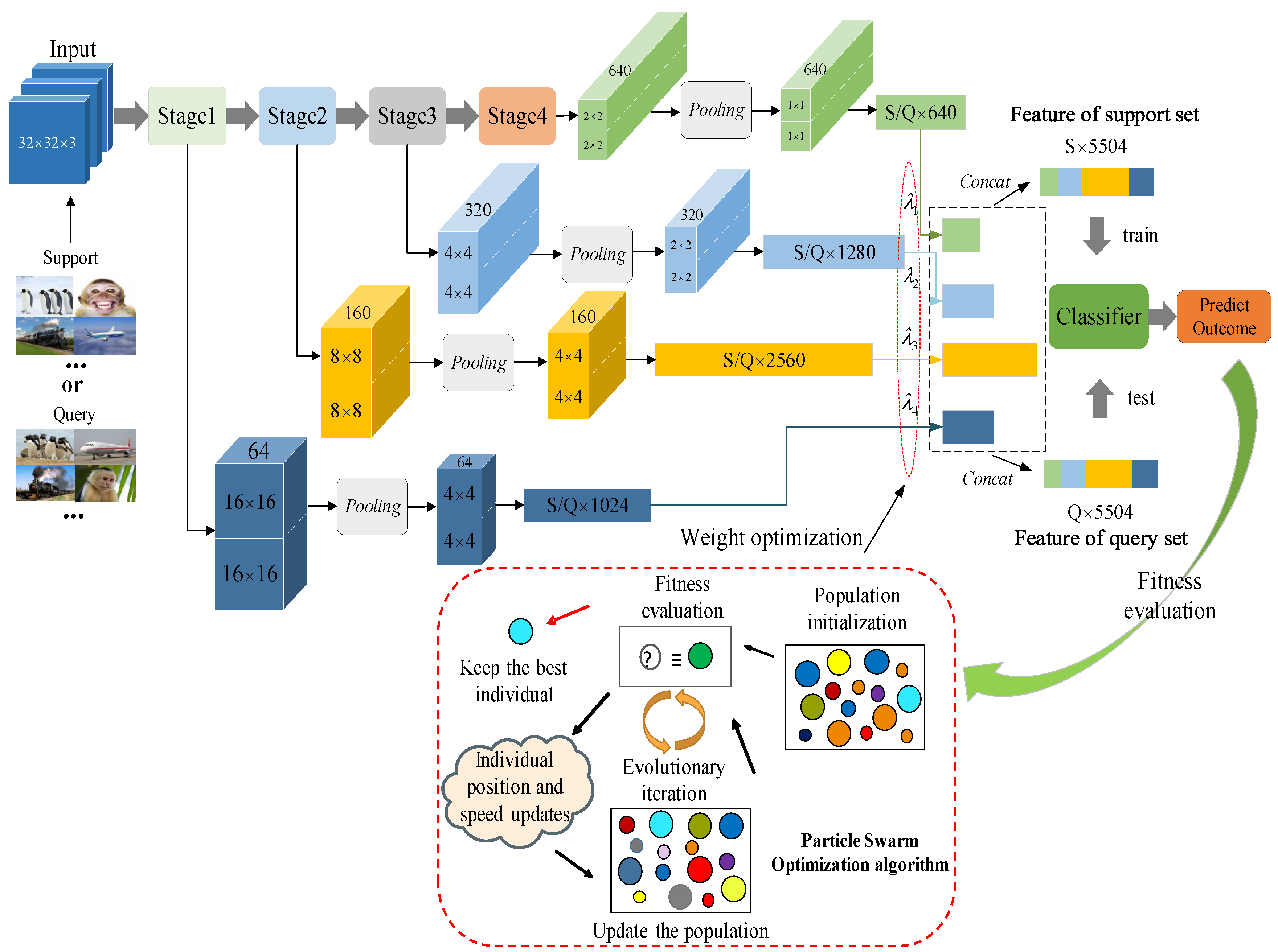
• We propose a meta-learning method based on adaptive feature fusion and weight optimization. The adaptive feature fusion method is used to train and test classifiers by fusing features from each stage of the embedding model, and the feature fusion weight is optimized by combining the classifier’s prediction results.
• In terms of the feature fusion method, we propose a novel feature splicing strategy: the output features of each stage are pooled and flattened, and then unified in a certain dimension. Feature splicing is carried out in this dimension. In the splicing process, the weight of each stage feature is different.
• For the optimization of the feature fusion weights, we combine the optimization algorithm with meta-learning and propose the use of a particle swarm optimization algorithm [27,28] to optimize the weights of the features at each stage of the embedding model. In addition, we use the parallel structure of the computer to optimize the feature fusion weights of multiple groups simultaneously to improve the algorithm’s efficiency.

In this paper, the proposed method is compared with the current state-of-the-art meta-learning methods. The experimental results show that the proposed method is effective and reliable.

2. Related Works

Meta-learning is the use of prior knowledge. Human beings can distinguish a category of objects only after seeing a few pictures. The focus of meta-learning research is how to equip the computer with such an ability. According to the utilization of prior knowledge, meta-learning can be divided into three directions, as shown below:

2.1. Metric-Based Meta-Learning

Metric-based meta-learning takes training data as prior knowledge. Koch et al. [7] used the Siamese network. After feature extraction, the confidence interval of each pair is predicted through the distance between testing and training samples, and the classification of the testing sample is judged. Prototypical Networks [8] determine the prototype representations of each class using the training sample and then calculates the distance between the testing sample and the prototype representations. In contrast to the first two, Relation Networks [9] introduce an attention mechanism, splicing feature extracted from both the support and query samples for discrimination and calculation of relational scores. Vinyals et al. [10] uses an attention mechanism, extracting features from support and query samples and calculating attention from each sample. GEFS [23] trains a well-performing embedding model on the meta-training set and then uses a machine learning model to metric the features extracted from the last stage of the embedding model.

2.2. External Memory-Based Meta-Learning

Meta-learning based on external memory introduces external memory through a new approach. The external memory was modified through a training sample, which was subsequently utilized as prior knowledge during the test. Santoro et al. [13] proposed a meta-learning algorithm for few-shot learning: for the model requiring strong generalization performance, the deep network model will result in the over-fitting of some tasks. Therefore, the external memory space is used to record information to complete the few-shot learning task combined with the neural network’s long-term memory ability. Meta-networks [14] used meta-learning to solve few-shot tasks and proposed MetaNet, composed of a basic and a meta-learner with extra memory. The training process of the network includes obtaining meta-information, fast weight generation, and slow weight optimization, learning a cross-task meta-level knowledge, and realizing fast parameterization of generalization tasks.

2.3. Initialization Method Based on Strong Generalization

The initialization method based on generalization introduces prior knowledge during model initialization. Model-Agnostic Meta-Learning (MAML) [17] aims to find a set of initialization parameters of the model that will allow the model to obtain good results by learning from a small number of samples. The main idea of MAML is to separate the task data used in optimizing network parameters from optimizing loss function to improve generalization performance. Reptile [20] is similar to MAML in that it optimizes in the direction of relatively superior tasks, while Reptile descends in the optimal direction of each task one by one and finally approximates to the position of relatively superior tasks. MAML is a meta-learning branch with great potential, and other methods such as Auto-Meta [29], MetaNAS [30], DEML [31] have emerged as a result of it.

3. Method

This section reviews the relevant preliminary knowledge of meta-learning and embedding model-based meta-learning before introducing our method. The method mainly includes feature fusion, weight optimization, and classifier training and testing. More on this below.

3.1. Meta-Learning Knowledge

The meta-learning datasets are divided into meta-training, meta-evaluation, and meta-testing sets. The image types of each set are mutually exclusive. A meta-training set is defined as $M={\left\{\right(D_i^{train},D_i^{test}\left)\right\}}_{i=1}^I$, and meta-evaluation set and meta-testing set are defined as $C={\left\{\right(D_j^{train},D_j^{test}\left)\right\} }_{j=1}^J$ and $D={\left\{\right(D_k^{train},D_k^{test}\left)\right\} }_{k=1}^K$ respectively. The tuple $(D_i^{train},D_i^{test})$ describes a training task and a testing task. Training examples $D^{train}=\left\{\right(x_t,y_t{\left)\right\} }_{t=1}^T$ and testing examples $D^{test}=\left\{\right(x_q,y_q{\left)\right\} }_{q=1}^Q$ are sampled from the same distribution.

Firstly, the embedding model is trained. The meta-training set combines all individual tasks together and defines as:

$$D^{combine}=\{D_1^{train},D_2^{train}......D_I^{train}\}$$

(1)

An effective embedding model $\varphi$ is defined as:

$$\varphi =arg\underset{\varphi }{min}{L}^{ce}(D^{combine};\varphi )$$

(2)

$L^{ce}$ represents the cross-entropy loss function (Figure 2). The cross-entropy loss function is a loss function for classification problems and is generally used in conjunction with the sofmax function. We use p(x) to denote the true distribution of the input samples and q(x) to denote the distribution predicted by the model, the cross-entropy loss function can be expressed as:

$$H(p,q)=D_{KL}(p||q)+H(p(\mathrm{x}))$$

(3)

$$D_{KL}(p||q)={\displaystyle \sum _{i=1}^{count}p({\mathrm{x}}_i)\log (p({\mathrm{x}}_i)/q({\mathrm{x}}_i))}$$

(4)

$$H(p(\mathrm{x}))=-{\displaystyle \sum _{i=1}^{count}p({\mathrm{x}}_i)\log (p({\mathrm{x}}_i))}$$

(5)

where count denotes the number of categories. $D_{KL}(p||q)$ denotes the Kullback–Leibler divergence, which measures the difference between p(x) and q(x). $H(p(\mathrm{x}))$ denotes the information entropy. Since the input samples and their labels are deterministic, the information entropy is a constant, so minimizing the Kullback–Leibler divergence can be translated into minimizing the cross-entropy loss function. Therefore, the cross-entropy loss function is often used as a loss function in machine learning

Then, a classifier A is given by $y_{\ast }=f_{\theta }({\mathit{x}}_{\ast })$, ${\mathit{x}}_{\ast }$ represents the feature extracted by $\varphi$. For a task $(D_j^{train},D_j^{test})$, train the classifier on $D_j^{train}$ and test the classifier on $D_j^{test}$. A can be represented as a multinomial logistic regression classifier, and its parameter $\theta =\{\mathit{W},\mathit{b}\}$ includes weight term $\mathit{W}$ and deviation term b, which can be expressed by the following formula:

$$\theta =arg\underset{\{\mathit{W},\mathit{b}\}}{min}{\displaystyle \sum _{t=1}^T{L}_t^{ce}(\mathit{W}{f}_{\varphi }({\mathit{x}}_t)+b,y_t)}+R(\mathit{W},\mathit{b})$$

(6)

where R is the regularization term.

3.2. Feature Fusion

This section describes the feature fusion method. In convolutional neural networks, the shallow feature contains a lot of low-level information. It is more concerned with details, while the deep feature contains a lot of high-level information and is more concerned with semantics. In Feature Pyramid Network [24], the input image is deeply convolved first, then the feature output from stages 2 and 4 are added, and the obtained results are fed into stage 5 to obtain strong semantic information and improve detection performance. In this work, the adaptive feature fusion method is used to obtain strong expression features to mine and effectively utilize different stages’ information.

First of all, the meta training set is used for training according to GEFS [23] to obtain a good embedding model, as depicted in Figure 3.

After obtaining a good embedding model, the N-way K-shot strategy on the meta-evaluation set/meta-testing set is used to obtain the support set and the query set. The embedding model is used to extract the features of the support and query sets. To obtain good performance feature, features are output and pooled at each stage of the embedding model. The calculations are as follows:

$${\tilde{\mathit{f}}}_l=Pooling(laye{r}_l({\mathit{x}}_i))$$

(7)

where ${\tilde{\mathit{f}}}_l$ represents the output features of each stage after pooling. Pooling () represents pooling operation, and $laye{r}_l({\mathit{x}}_i)$ represents the feature extraction operation of the l-th stage.

The output features of each stage are transformed to the same dimension. The features are spliced according to this dimension to achieve a combination of low-level and high-level information and obtain strong semantic information. The calculations are as follows:

$${\mathit{f}}_l=Resize({\tilde{\mathit{f}}}_l)$$

(8)

Resize () in Equation (8) indicates the dimensional unity of the feature.

Furthermore, the predicted values are obtained and compared using the output feature of each stage. It is concluded that the features of each stage have different influences on meta-learning accuracy. Therefore, during the feature fusion, the features of each stage have different weights, as shown in Equation (9).

$$\mathit{F}=Concat({\lambda }_1{\mathit{f}}_1,{\lambda }_2{\mathit{f}}_2,{\lambda }_3{\mathit{f}}_3,{\lambda }_4{\mathit{f}}_4)$$

(9)

where $\lambda$ represents the weight of the output feature with a different stage in feature fusion. Concat () indicates feature splicing, and $\mathit{F}$ represents the fusion feature with a different weight.

After the feature fusion process is complete, the fused features are fed into the classifier for prediction:

$$y^{predict}=Classifier({\mathit{F}}_{last})$$

(10)

Classifier () represents the classifier. The classifier training process is the same as the testing process.

The method of feature fusion is shown in Figure 4.

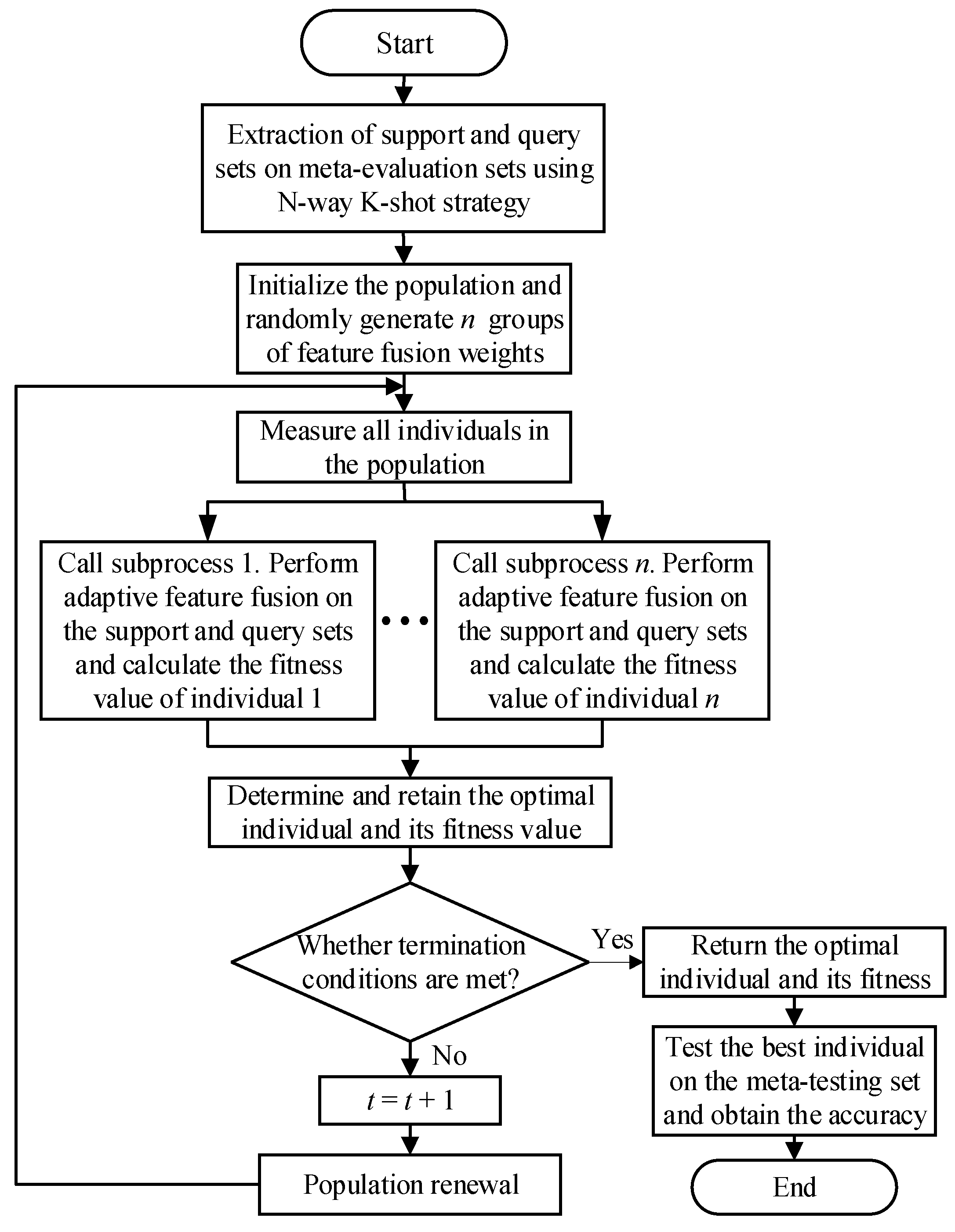
3.3. Weight Optimization

The particle swarm optimization (PSO) [27,28] algorithm is used in weight optimization. First, the weight optimization is carried out on the meta-evaluation set, and the optimal feature fusion weight is found by the optimization algorithm used in meta-testing. The particle swarm optimization algorithm is discussed in detail below.

PSO is derived from the study of flock predation behavior and has the characteristics of evolution and swarm intelligence. The algorithm stores the information of the optimal global position and the known optimal local position, which has a good effect on fast convergence and avoids premature falling into the optimal local solution. However, it is easy for the standard particle swarm algorithm to fall into local optimum, and to overcome this problem, we use an adaptive inertia weight strategy that relates the change in inertia weight to the change in the particle’s own fitness, and we use the fitness variance to determine whether the algorithm falls into local optimum. If the algorithm falls into local optimum, a disturbance mechanism is used to generate new particles and replace the particles with the worst fitness in the population when the algorithm stalls, thus allowing the particles to jump out of the local optimum. Compared to other optimization algorithms, the particle swarm optimization algorithm has memory, all particles in the algorithm retain a better solution and the particles are only updated by internal velocity, making the algorithm easier to implement with fewer parameters. Therefore, this paper uses the particle swarm optimization algorithm to optimize the feature fusion weights. Our algorithm framework is shown in Figure 5.

(1) Population initialization $Q(t_0)={\{Q_i(t_0)\}}_{i=1}^n$, where $Q_i(t_0)$ represents the i-th individual of the $t_0$ generation in the population. $t_0$ is the initial generation and n is the total number of individuals in the population. Each individual has an initial position $X_{t_0}^i$ and an initial velocity $V_{t_0}^i$ at the beginning. Each group weight of feature fusion corresponds to an individual, and population initialization corresponds to the initialization of n group weight of ${\lambda }^i={\{{\lambda }_1^i,{\lambda }_2^i,{\lambda }_3^i,{\lambda }_4^i\}}_{i=1}^n$ of feature fusion.

(2) Each individual in the population is measured, and the individual solution can be expressed as $P(t)={(P_i(t))}_{i=1}^n$, where $P_i(t)$ represents the solution of the i-th individual in the t generation population.

(3) $P_i(t)$ is evaluated by the fitness function. Given that the meta-evaluation set $C={\left\{\right(D_j^{train},D_j^{test}\left)\right\} }_{j=1}^J$, $D_j^{train}$ is used to train the classifier, $D_j^{test}$ is used to test the classifier, and the optimization process of each individual is set up as a thread that the computer can execute using the parallel computing method. The meta-learning accuracy of the classifier to the meta-evaluation set is defined as the fitness function of the population:

$$Fitness(P_i(t))=Acc(C)$$

(11)

where $Acc(C)$ represents the accuracy of the meta-evaluation set, and the calculation method can be expressed as:

$$Acc(C)=\frac{Predictthecorrectsamplesize}{Thetotalnumberofsamples}\times 100\%$$

(12)

(4) The optimal individual is determined and retained. The optimal individuals and their fitness values were retained as the target of subsequent evolution. If the population position stabilizes, the algorithm ends; otherwise, t $\leftarrow$ t + 1, and the next step is performed.

(5) According to the fitness function value $Fitness(P_i(t))$ and population renewal strategy, the position $X_t^i$ and velocity $V_t^i$ of the previous generation of individuals were updated to obtain the next generation of population $\mathrm{Q}(t+1)=\{Q_1(t+1),Q_2(t+1)\cdots Q_n(t+1)\}$ and return to step (2). The population renewal strategy is as follows:

$$V_{t+1}^i=w{V}_t^i+c1r1(P_{best}^i-X_t^i)+c2r2(g_{best}-X_t^i)$$

(13)

$$X_{t+1}^i=X_t^i+V_t^i$$

(14)

where $P_{best}^i$ represents the optimal position experienced by the i-th individual and $g^{best}$ represents the optimal position experienced by the whole population. c1 and c2 are acceleration constants used to adjust the learning step, r1 and r2 are random functions with values in the range of [0, 1], and w is the inertia weight.

When the optimization method is complete, the optimal fusion weight is used to test in the meta-testing set. Input ${\mathit{F}}^{last}$ into the classifier for testing, and the calculation formula is as follows:

$$y^{predict}=Classifier({\mathit{F}}_{last})$$

(15)

The training process of the classifier is the same as the testing process, which uses Equation (15). The pseudo-code of adaptive feature fusion and weight optimization algorithm is shown in Algorithm 1.

Algorithm 1 Adaptive feature fusion and weight optimization algorithm pseudo-code

Input: the meta-evaluation set $C={\{(D_j^{train},D_j^{test})\}}_{j=1}^J$;         1: Initialize t to 1;         2: For i = 1: n do               3: Population initialization $Q(t_0)={\{Q_i(t_0)\}}_{i=1}^n$;               4: The individual solution $P(t)={\{P_i(t)\}}_{i=1}^n$ and fitness function was measured by multi-threads.                   Fitness function evaluation $Fitness(P_i(t))=Acc(C)$; 5: Determine and retain the optimal individual and its fitness value; 6: End for 7: while the population position has not reached stability do 8: For i = 1: n    do 9: Equation (13) and Equation (14) were used to update population individuals                  $\mathrm{Q}(t+1)=\{Q_1(t+1),Q_2(t+1)\cdots Q_n(t+1)\}$; 10: End for 11: For i = 1: n    do               12: Perform steps 4 and 5; 13: End for 14: t $\leftarrow$ t + 1; 15: End while          Output: the optimal individual;

3.4. Meta-Classifier

After a good embedding model is obtained, the classifier will be trained and tested using the extracted features. The classifiers used for classification tasks include nearest neighbor algorithm, Bayesian algorithm, logistic regression, and support vector machine. At present, the multinomial logistic regression model is used primarily for meta-classification. Logistic regression is a regression model that narrows the prediction range and limits the predicted value to the range [0, 1]. Multinomial logistic regression improves binary logistic regression that can be generalized to train and predict multiple classification problems. The algorithm trains a multinomial logistic regression model for the multi-classification problem, including M-1 binary regression models. Given a data point, M-1 models are run simultaneously, and the category with the highest probability is chosen as the prediction category.

4. Experimental Results

This section describes the experimental setup and numerous results.

4.1. Dataset

We perform experiments on the three widely used few-shot image recognition datasets and the Miner Unsafe Behavior dataset (MUB). MiniImageNet [10] is the derivative of ImageNet [32], and CIFAR-FS [33] and FC100 [34] are extracted from CIFAR-100 [35,36]. The Miner Unsafe Behavior dataset is a video dataset established by this research team that contains a wide range of miners’ unsafe behaviors.

The miniImageNet dataset is a widely used dataset in few-shot learning. The dataset is extracted from ImageNet and contains 100 classes, each containing 600 images with a resolution of 84 × 84 pixels. Out of the total classes, 64 are used as a meta-training set, 16 as a meta-evaluation set, and 20 as a meta-testing set.

The CIFAR-FS dataset, fully called CIFAR100 few-shot dataset, is extracted from the standard CIFAR100. It contains 100 classes in total, each containing 600 images with a resolution of 32 × 32 pixels, with 60,000 images. Out of the total classes, 64 are used as a meta-training set, 16 as a meta-evaluation set, and 20 as a meta-testing set.

The FC100 dataset is another subset of CIFAR100, containing 100 classes, each containing 600 images having a resolution of 32 × 32 pixels, with a total of 60,000 images. However, FC100 is divided into super-classes rather than classes. Among them, 12 super-classes (60 classes) are used as meta-training sets, 4 super-classes (20 classes) are used as meta-evaluation sets, and 4 super-classes (20 classes) are used as meta-testing sets.

The MUB dataset contains 51 classes of miners’ unsafe behaviors and 1530 sets of video actions. Each behavior consists of 30 video actions performed three times by 10 members of the research team. Out of the total classes, 31 are used as a meta-training set, 10 as a meta-evaluation set, and 10 as a meta-testing set.

4.2. Setup

Server configuration: In terms of server configuration, a server with 32 GB memory, two GTX-1080ti graphics processors, and a Windows-10 operating system was used for experimental verification. In terms of architecture, the PyTorch deep learning architecture is used [37].

Optimization setup: For the three widely used few-shot image recognition datasets, Stochastic Gradient Descent (SGD) optimizer with a momentum of 0.9 and a weight decay of 5 × 10⁻⁴ were used. Each batch consists of 64 samples. The learning rate was initialized to 0.05 and decayed three times with a factor of 0.1, once at the start of training, once at the 30th epoch, and once at the 60th epoch. The exception is miniImageNet, in which only two decays are made, and the third decays has no effect. MiniImageNet used 100 epochs, while CRFAR-FS and FC100 used 90 epochs. For the MUB dataset, we used SGD optimizer with a momentum of 0.9 and a weight decay of 1 × 10⁻³. Each batch consists of 16 samples. The learning rate is initialized to 0.2 and decayed four times by a factor of 0.1. The MUB dataset used 150 epochs.

Backbone architecture: Based on previous research, for the three public datasets, ResNet12 was experimentally selected as the backbone network which consisted of four residual blocks. After the first three blocks, 4 × 4 self-adaptive pooling, 4 × 4 self-adaptive pooling, and 2 × 2 self-adaptive pooling were adopted, respectively, and 1 × 1 self-adaptive pooling was adopted after the last block. In subsequent experiments, SEResNet-12 was used as the backbone network for comparison, and the residual blocks of the two backbones are shown in Figure 6. SEResNet-12 adds extrusion and excitation mechanisms based on ResNet-12. The first and the second layers are fully connected to reduce dimensionality, resulting in a significant reduction in the number of parameters and computation. For the MUB dataset, MobineNet-V2 was selected as the backbone, which contained two convolutional layers at the beginning and end, as well as several modules. The experiment output is the features in specific modules for feature fusion.

Data augmentation: During the training of the embedding model, random clipping, color dithering, and random horizontal flip [38] are used for data augmentation on the three public datasets. For the MUB dataset, data augmentation methods such as random horizontal flipping and center cropping are used to enhance the generalization performance of the embedding model.

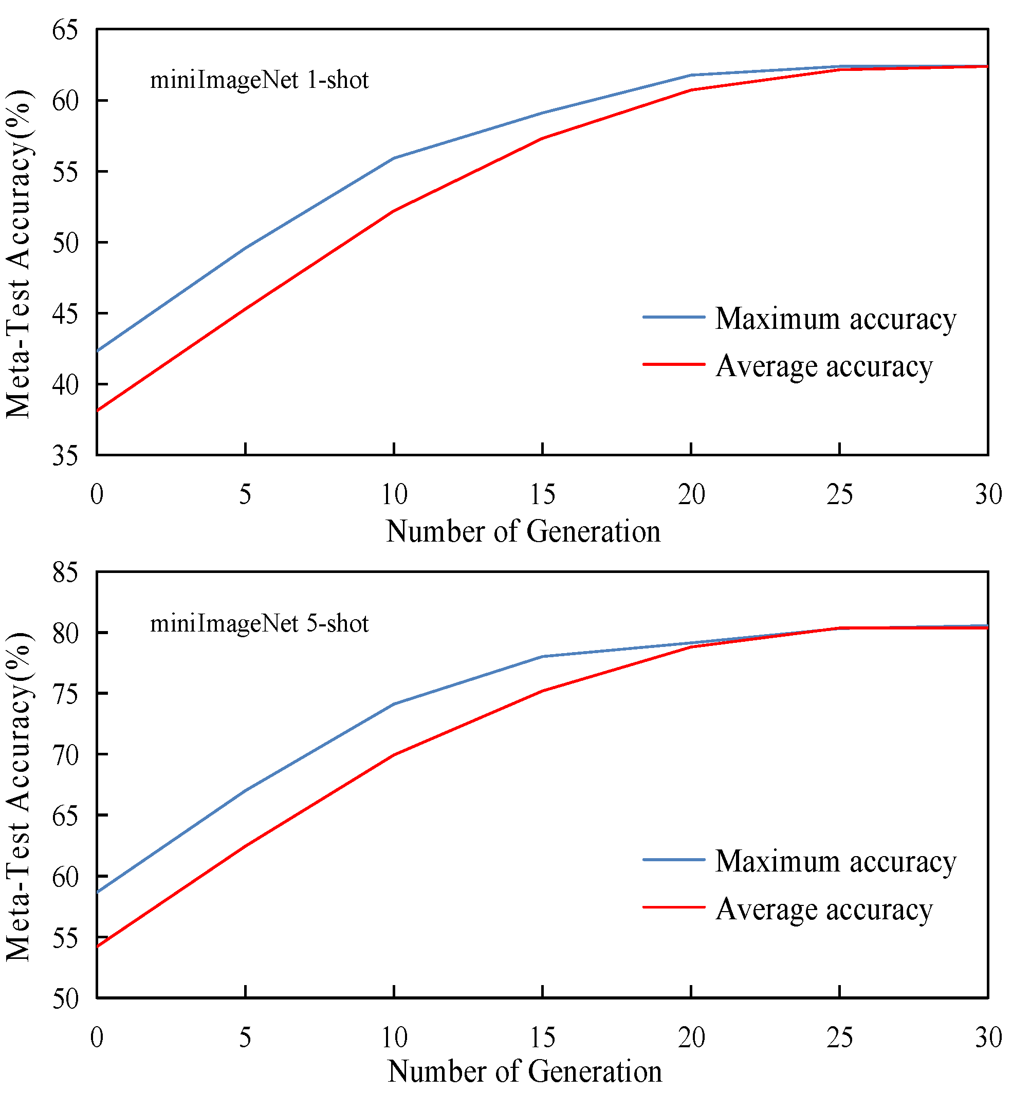
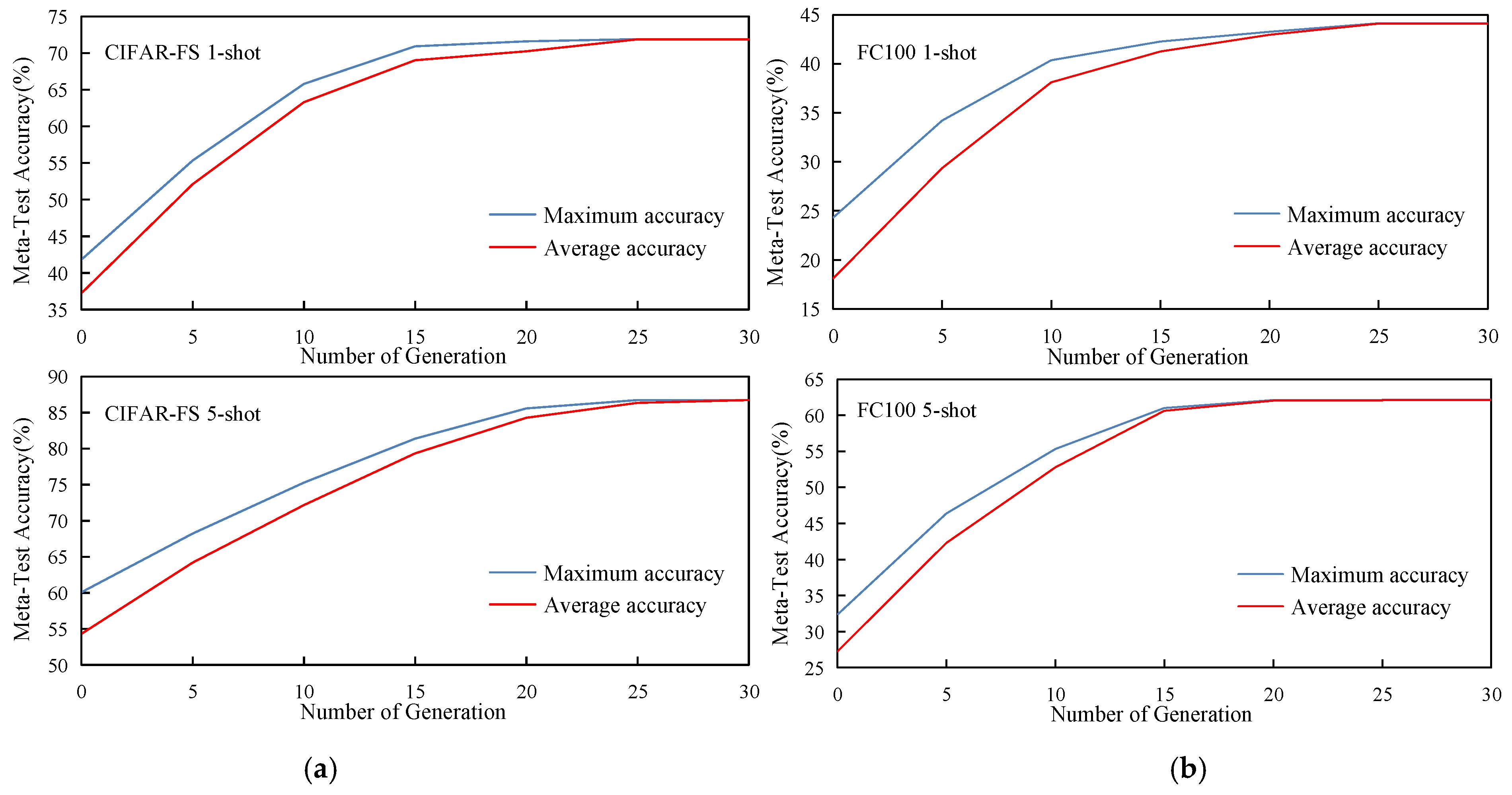
4.3. Results and Discussion

We conduct experiments on the miniImageNet dataset. The number of random seeds was fixed to ensure the verifiability of the experiment. The particle swarm optimization algorithm was used to optimize the weight of adaptive feature fusion on the meta-evaluation set. The population was set up with 10 individuals, and the iterations were set at 30 generations. After finding the optimal weight, it was used for the meta-testing. The results of the experiment are shown in

Table 1. Experiments were conducted on the miniImageNet dataset and our approach was compared with existing methods. Average meta-learning classification accuracies (%) with 95% confidence intervals on miniImageNet meta-test splits. a-b-c-d denotes the size of the layer in the backbone.

Model	Backbone	miniImageNet 5-Way
		1-Shot	5-Shot
MAML [17]	32-32-32-32	48.70 ± 1.84	63.11 ± 0.92
Matching Networks [10]	64-64-64-64	43.56 ± 0.84	55.31 ± 0.73
IMP [39]	64-64-64-64	49.2 ± 0.7	64.7 ± 0.7
Prototypical Networks [8]	64-64-64-64	49.42 ± 0.78	68.20 ± 0.66
TAML [18]	64-64-64-64	51.77 ± 1.86	66.05 ± 0.85
SAML [40]	64-64-64-64	52.22 ± n/a	66.49 ± n/a
GCR [41]	64-64-64-64	53.21 ± 0.80	72.34 ± 0.64
KTN [42]	64-64-64-64	54.61 ± 0.80	71.21 ± 0.66
PARN [43]	64-64-64-64	55.22 ± 0.84	71.55 ± 0.66
Dynamic Few-shot [44]	64-64-128-128	56.20 ± 0.86	73.00 ± 0.64
Relation Networks [9]	64-64-128-128	50.44 ± 0.82	65.32 ± 0.70
R2D2 [33]	96-192-384-512	51.2 ± 0.6	68.8 ± 0.1
SNAIL [45]	ResNet-12	55.71 ± 0.99	68.88 ± 0.92
AdaResNet [46]	ResNet-12	56.88 ± 0.62	71.94 ± 0.57
TADAM [34]	ResNet-12	58.50 ± 0.30	76.70 ± 0.30
Shot-Free [47]	ResNet-12	59.04 ± n/a	77.64 ± n/a
TEWAM [48]	ResNet-12	60.07 ± n/a	75.90 ± n/a
MTL [49]	ResNet-12	61.20 ± 1.80	75.50 ± 0.80
Variational FSL [50]	ResNet-12	61.23 ± 0.26	77.69 ± 0.17
MetaOptNet [38]	ResNet-12	62.64 ± 0.61	78.63 ± 0.46
Diversityw/Cooperation [51]	ResNet-18	59.48 ± 0.65	75.62 ± 0.48
Fine-tuning [52]	WRN-28-10	57.73 ± 0.62	78.17 ± 0.49
LEO-trainval [53]	WRN-28-10	61.76 ± 0.08	77.59 ± 0.12
GEFS [23]	ResNet-12	62.02 ± 0.63	79.64 ± 0.44
Ours	ResNet-12	62.55 ± 0.81	80.57 ± 0.57

In the 1-shot strategy, the proposed method results are similar to the state-of-the-art MetaOptNet [38] and better than GEFS [23]. The proposed method outperforms all others in the five-shot strategy. Experiments show that the method is both effective and reliable.

To demonstrate the effectiveness of the particle swarm optimization algorithm in weight optimization, each generation’s optimal feature fusion weights found on the meta-evaluation set are used for meta-testing. Figure 7 shows the relationship between the maximum accuracy and average accuracy of miniImageNet and the generation in meta-testing under the one-shot and five-shot strategies. The particle swarm optimization algorithm has been found to be both effective and reliable.

The method is validated on FC100 and CIFAR-FS. The population was set up with 10 individuals, and the iterations were set at 30 generations. The results of the experiment are shown in

Table 2. Experiments were performed on CIFAR-FS and FC100 and our approach was compared with existing methods. Average meta-learning classification accuracies (%) with 95% confidence intervals on CIFAR-FS and FC100 meta-test splits. a-b-c-d denotes the size of the layer in the backbone.

Model	Backbone	CIFAR-FS 5-Way		FC100 5-Way
		1-Shot	5-Shot	1-Shot	5-Shot
MAML [17]	32-32-32-32	58.9 ± 1.9	71.5 ± 1.0	-	-
Prototypical Networks [8]	64-64-64-64	55.5 ± 0.7	72.0 ± 0.6	35.3 ± 0.6	48.6 ± 0.6
Relation Networks [9]	64-64-128-128	55.0 ± 1.0	69.3 ± 0.8	-	-
R2D2 [33]	96-192-384-512	65.3 ± 0.2	79.4 ± 0.1	-	-
TADAM [34]	ResNet-12	-	-	40.1 ± 0.4	56.1 ± 0.4
Shot-Free [47]	ResNet-12	69.2 ± n/a	84.7 ± n/a	-	-
TEWAM [48]	ResNet-12	70.4 ± n/a	81.3 ± n/a	-	-
Prototypical Networks [8]	ResNet-12	72.2 ± 0.7	83.5 ± 0.5	37.5 ± 0.6	52.5 ± 0.6
MetaOptNet [38]	ResNet-12	72.6 ± 0.7	84.3 ± 0.5	41.1 ± 0.6	55.5 ± 0.6
GEFS [23]	ResNet-12	71.5 ± 0.8	86.0 ± 0.5	42.6 ± 0.7	59.1 ± 0.6
Ours	ResNet-12	71.91 ± 0.85	86.77 ± 0.63	44.16 ± 0.77	62.17 ± 0.72

. The results of the one-shot strategy outperforms GEFS [23] for CIFAR-FS, whereas the results of the five-shot strategy achieve the best performance. For FC100, our approach achieved the best performance for both one-shot and five-shot strategies.

The effectiveness of particle swarm optimization algorithm has also been proven on FC100 and CIFAR-FS. Figure 8a shows the relationship between the maximum accuracy and average accuracy of the CIFAR-FS dataset and the generation in meta-testing under the one-shot and five-shot strategies. Figure 8b displays the relationship between the maximum accuracy and average accuracy of the FC100 dataset and the generation in meta-testing under the one-shot and five-shot strategies.

To further verify the effectiveness of the method, we performed experiments on the Miner Unsafe Behavior dataset by extracting video key frames. Random seed number was fixed to ensure the experiment verifiability. The population was set up with 10 individuals and the iterations were set at 20 generations. The experimental results obtained by comparing the meta-learning accuracy before and after feature fusion are shown in

Table 3. We conduct experiments on the MUB dataset. Average meta-learning classification accuracies (%) with 95% confidence intervals on MUB meta-test splits.

Model	Backbone	MUB 5-Way
		1-Shot	5-Shot
Ours-simple	MobileNet-V2	39.57 ± 2.42	52.92 ± 2.19
Ours-fuse	MobileNet-V2	49.48 ± 2.05	68.25 ± 2.03

. This method achieves good performance.

4.4. Ablation Study

4.4.1. Comparison of Different Feature Fusion Methods

Generally speaking, a better feature fusion method can achieve better results. In this work, in order to further verify that the proposed method is state-of-the-art, comparative experiments are carried out on multiple feature fusion methods. The feature fusion methods chosen by the study include: directly fusing the output features by each stage of the embedding model according to the same size of channels, without flattening the output features; performing addition operations on the features output by stage 1 and stage 2 and inputting them into stage 3, in a similar way to [24]. The experimental results in

Table 4. Comparison of different feature fusion methods on the miniImageNet dataset. “Ours-channels” denotes fusing features directly by the same size of channels. “Ours-addition” denotes summing features from different stages and feeding them to other stages. Average meta-learning classification accuracies (%) with 95% confidence intervals on miniImageNet meta-test splits.

Model	Backbone	miniImageNet 5-Way
		1-Shot	5-Shot
Ours-channels	ResNet-12	62.25 ± 0.61	80.14 ± 0.42
Ours-addition	ResNet-12	62.16 ± 0.58	79.83 ± 0.51
Ours-fuse	ResNet-12	62.55 ± 0.81	80.57 ± 0.57

and

Table 5. Comparison of different feature fusion methods on CIFAR-FS and FC100. “Ours-channels” denotes fusing features directly by the same size of channels. “Ours-addition” denotes summing features from different stages and feeding them to other stages. Average meta-learning classification accuracies (%) with 95% confidence intervals on CIFAR-FS and FC100.

Model	Backbone	CIFAR-FS 5-way		FC100 5-Way
		1-Shot	5-Shot	1-Shot	5-Shot
Ours-channels	ResNet-12	71.72 ± 0.8	86.32 ± 0.64	42.92 ± 0.71	59.8 ± 0.54
Ours-addition	ResNet-12	71.67 ± 0.72	86.21 ± 0.59	42.81 ± 0.75	59.42 ± 0.67
Ours-fuse	ResNet-12	71.91 ± 0.85	86.77 ± 0.63	44.16 ± 0.77	62.17 ± 0.72

show that the strategy of feature fusion according to the size of channels and the strategy of summing the output features of different stages and feeding them to other stages are inferior to the adaptive feature fusion method.

4.4.2. Comparison of Different Classifiers

The effects of different classifiers on the experiment were tested, and multiple classifiers were used for validation on three public datasets. The experimental classifiers include nearest neighbor classification, support vector machine, cosine similarity, and logistic regression. The experimental results are shown in

Table 6. Ablation experiments with classifiers. “NN” and “LR” denote nearest neighbor classifier and logistic regression. “Cosine” stands for cosine similarity.

Classifier	CIFAR-FS 5-Way		FC100 5-Way		miniImageNet 5-Way
	1-Shot	5-Shot	1-Shot	5-Shot	1-Shot	5-Shot
NN	68.9 ± 0.86	81.82 ± 0.67	42.41 ± 0.75	57.92 ± 0.74	61.03 ± 0.83	73.85 ± 0.65
SVM	71.32 ± 0.88	83.96 ± 0.75	40.89 ± 0.75	58.43 ± 0.76	58.16 ± 0.78	74.58 ± 0.64
Cosine	68.9 ± 0.86	81.82 ± 0.67	42.41 ± 0.75	57.92 ± 0.74	61.03 ± 0.83	73.85 ± 0.65
LR	71.91 ± 0.85	86.77 ± 0.63	44.16 ± 0.77	62.17 ± 0.72	62.55 ± 0.81	80.57 ± 0.57

. The performance of each classifier varies depending on the dataset, but the logistic regression classifier is better than other classifiers in the experiment; hence it is selected for subsequent research.

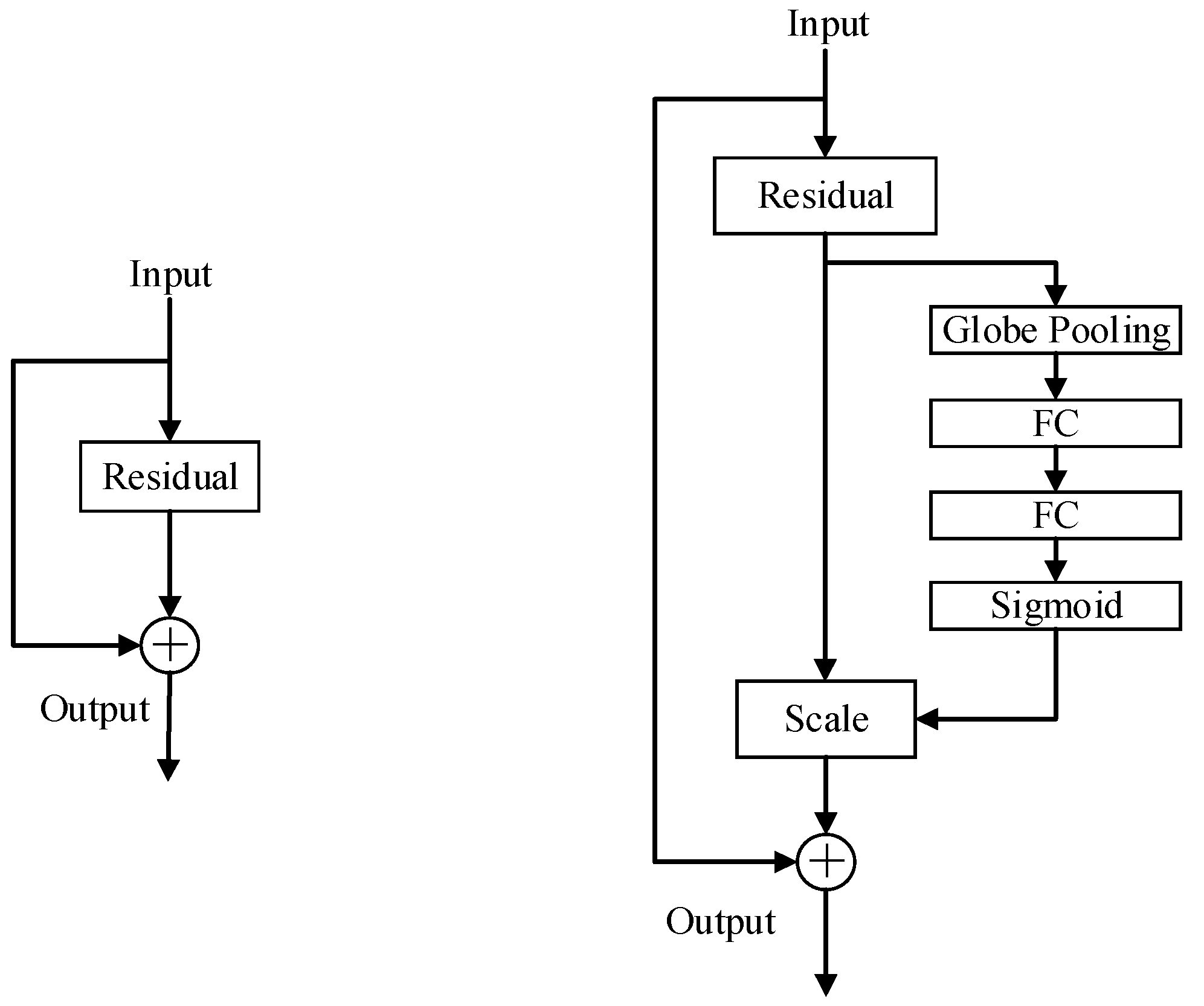
4.4.3. Comparison of Different Backbones

ResNet-12 is used as the backbone in the above experiments. To compare the performance of the algorithm under different backbone networks, ResNet-12 and SEResNet-12 are used in comparative experiments. Figure 6 shows the network structure of ResNet-12 and SEResNet-12. The experimental results are shown in

Table 7. Meta-learning accuracy of different backbones on CIFAR-FS and FC100.

Model	CIFAR-FS 5-Way		FC100 5-Way
	1-Shot	5-Shot	1-Shot	5-Shot
ResNet-12	71.91 ± 0.85	86.77 ± 0.63	44.16 ± 0.77	62.17 ± 0.72
SEResNet-12	72.31 ± 0.93	86.84 ± 0.59	44.58 ± 0.84	62.52 ± 0.68

and

Table 8. Meta-learning accuracy of different backbones on miniImageNet.

Model	miniImageNet 5-Way
	1-Shot	5-Shot
ResNet-12	62.55 ± 0.81	80.57 ± 0.57
SEResNet-12	62.81 ± 0.92	80.95 ± 0.62

. It can be concluded that the algorithm exhibits better performance under SEResNet-12, indicating that SEResNet-12 better represents the features of the samples.

4.4.4. Comparison of Different Optimization Algorithms

In this paper, to verify the impact of different optimization algorithms on the experimental results, we used quantum genetic algorithms (QGA) and particle swarm optimization algorithms for comparison. To ensure the accuracy of the experiments, the classifiers we used were all logistic regression classifiers, and the backbone network uniformly used ResNet12. The experimental results are shown in

Table 9. Meta-learning accuracy of different optimization methods on miniImageNet. QGA denotes Quantum Genetic Algorithm. PSO stands for Particle Swarm Optimization.

Optimization Method	Backbone	miniImageNet 5-Way
		1-Shot	5-Shot
QGA	ResNet-12	62.29 ± 0.71	80.05 ± 0.52
PSO	ResNet-12	62.55 ± 0.81	80.57 ± 0.57

and

Table 10. Meta-learning accuracy of different optimization methods on CIFAR-FS and FC100.

Optimization Method	Backbone	CIFAR-FS 5-Way		FC100 5-Way
		1-Shot	5-Shot	1-Shot	5-Shot
QGA	ResNet-12	71.72 ± 0.76	86.68 ± 0.94	44.02 ± 0.59	61.98 ± 0.64
PSO	ResNet-12	71.91 ± 0.85	86.77 ± 0.63	44.16 ± 0.77	62.17 ± 0.72

. It can be concluded that the results using the particle swarm optimization algorithm are slightly better than those of the quantum genetic algorithm, further confirming the reliability and stability of the particle swarm optimization algorithm.

5. Conclusions

In terms of the differences between the features of different stages of the convolutional neural networks and the impact of the features of different stages on the performance of the classifier, this paper proposes a meta-learning method based on adaptive feature fusion and weight optimization. This method merges different features of the low and high stages of the embedding model, and optimizes the feature fusion weights through the particle swarm algorithm; on this basis, this method optimizes the weights on the meta-evaluation set, and uses the obtained optimal fusion weights for the meta-test. The method was verified on the three widely used few-shot image recognition datasets and the MUB dataset produced by the research team. The results show that compared with the current mainstream meta-learning methods, the proposed method has achieved better performance. In future research, we intend to build on the research in this paper to explore the effect of the dimensionality of the features output by the pooling layer of the embedding model on the performance of the classifier. We attempt to vary the pooling dimension of the pooling layer at each stage of the embedding model, and hence the dimensionality of the output features at each stage. The pooling dimension of each stage and the feature fusion weights of each stage are jointly optimized by an optimization algorithm in the hope of further improving the performance of the classifier.

References

1. LeCun, Y.; Bengio, Y.; Hinton, G. Deep learning. Nature 2015, 521, 436–444. [Google Scholar] [CrossRef] [PubMed]
2. Voulodimos, A.; Doulamis, N.; Doulamis, A.; Protopapadakis, E. Deep learning for computer vision: A brief review. Comput. Intell. Neurosci. 2018, 2018, 1–13. [Google Scholar] [CrossRef] [PubMed]
3. Vanschoren, J. Meta-learning. In Automated Machine Learning; Springer: Cham, Switzerland, 2019; pp. 35–61. [Google Scholar]
4. Wang, Y.; Yao, Q.; Kwok, J.T.; Ni, L.M. Generalizing from a few examples: A survey on few-shot learning. ACM Comput. Surv. (CSUR) 2020, 53, 1–34. [Google Scholar] [CrossRef]
5. Vanschoren, J. Meta-learning: A survey. arXiv 2018, arXiv:1810.03548. [Google Scholar]
6. Chen, Y.; Liu, Z.; Xu, H.; Darrell, T.; Wang, X. Meta-baseline: Exploring simple meta-learning for few-shot learning. In Proceedings of the IEEE/CVF International Conference on Computer Vision, Sunnyvale, CA, USA, 25 October 2021; pp. 9062–9071. [Google Scholar]
7. Koch, G.; Zemel, R.; Salakhutdinov, R. Siamese neural networks for one-shot image recognition. In Proceedings of the ICML Deep Learning Workshop, Lille, France, 6–11 July 2015; Volume 2. [Google Scholar]
8. Snell, J.; Swersky, K.; Zemel, R.S. Prototypical networks for few-shot learning. arXiv 2017, arXiv:1703.05175. [Google Scholar]
9. Sung, F.; Yang, Y.; Zhang, L.; Xiang, T.; Torr, P.H.; Hospedales, T.M. Learning to compare: Relation network for few-shot learning. In Proceedings of the IEEE Conference on Computer Vision and Pattern Recognition, Salt Lake City, UT, USA, 18–22 June 2018; pp. 1199–1208. [Google Scholar]
10. Vinyals, O.; Blundell, C.; Lillicrap, T.; Wierstra, D. Matching networks for one shot learning. Adv. Neural Inf. Process. Syst. 2016, 29, 3630–3638. [Google Scholar]
11. Karlinsky, L.; Karlinsky, L.; Shtok, J.; Harary, S.; Marder, M.; Pankanti, S.; Bronstein, A.M. Repmet: Representative-based metric learning for classification and few-shot object detection. In Proceedings of the IEEE/CVF Conference on Computer Vision and Pattern Recognition, Long Beach, CA, USA, 15–20 June 2019; pp. 5197–5206. [Google Scholar]
12. Li, W.; Wang, L.; Xu, J.; Huo, J.; Gao, Y.; Luo, J. Revisiting local descriptor based image-to-class measure for few-shot learning. In Proceedings of the IEEE/CVF Conference on Computer Vision and Pattern Recognition, Long Beach, CA, USA, 16–17 June 2019; pp. 7260–7268. [Google Scholar]
13. Santoro, A.; Bartunov, S.; Botvinick, M.; Wierstra, D.; Lillicrap, T. Meta-learning with memory-augmented neural networks. In Proceedings of the International Conference on Machine Learning PMLR, York City, NY, USA, 19–24 June 2016; pp. 1842–1850. [Google Scholar]
14. Munkhdalai, T.; Yu, H. Meta networks. In Proceedings of the International Conference on Machine Learning PMLR, Sydney, Australia, 6–11 August 2017; pp. 2554–2563. [Google Scholar]
15. Cai, Q.; Pan, Y.; Yao, T.; Yan, C.; Mei, T. Memory matching networks for one-shot image recognition. In Proceedings of the IEEE Conference on Computer Vision and Pattern Recognition, Salt Lake City, UT, USA, 18–22 June 2018; pp. 4080–4088. [Google Scholar]
16. Kaiser, Ł.; Nachum, O.; Roy, A.; Bengio, S. Learning to remember rare events. arXiv 2017, arXiv:1703.03129. [Google Scholar]
17. Finn, C.; Abbeel, P.; Levine, S. Model-agnostic meta-learning for fast adaptation of deep networks. In Proceedings of the International Conference on Machine Learning PMLR, Sydney, Australia, 6–11 August 2017; pp. 1126–1135. [Google Scholar]
18. Jamal, M.A.; Qi, G.-J. Task agnostic meta-learning for few-shot learning. In Proceedings of the IEEE/CVF Conference on Computer Vision and Pattern Recognition, Sydney, Australia, 6–11 August 2019; pp. 11719–11727. [Google Scholar]
19. Li, Z.; Zhou, F.; Chen, F.; Li, H. Meta-sgd: Learning to learn quickly for few-shot learning. arXiv 2017, arXiv:1707.09835. [Google Scholar]
20. Nichol, A.; Achiam, J.; Schulman, J. On first-order meta-learning algorithms. arXiv 2018, arXiv:1803.02999. [Google Scholar]
21. Ye, H.-J.; Hu, H.; Zhan, D.-C.; Sha, F. Learning embedding adaptation for few-shot learning. arXiv 2019, arXiv:1812.03664. [Google Scholar]
22. Hao, F.; Cheng, J.; Wang, L.; Cao, J. Instance-level embedding adaptation for few-shot learning. IEEE Access 2019, 7, 100501–100511. [Google Scholar] [CrossRef]
23. Tian, Y.; Wang, Y.; Krishnan, D.; Tenenbaum, J.B.; Isola, P. Rethinking few-shot image classification: A good embedding is all you need? In Proceedings of the Computer Vision–ECCV 2020: 16th European Conference, Glasgow, UK, 23–28 August 2020; Springer: Berlin/Heidelberg, Germany, 2020; Volume 16 (Pt XIV), pp. 266–282. [Google Scholar]
24. Lin, T.-Y.; Dollár, P.; Girshick, R.; He, K.; Hariharan, B.; Belongie, S. Feature pyramid networks for object detection. In Proceedings of the IEEE Conference on Computer Vision and Pattern Recognition, Honolulu, HI, USA, 21–26 June 2017; pp. 2117–2125. [Google Scholar]
25. Deng, C.; Wang, M.; Liu, L.; Liu, Y.; Jiang, Y. Extended feature pyramid network for small object detection. IEEE Trans. Multimed. 2021, 24, 1968–1979. [Google Scholar] [CrossRef]
26. Selvaraju, R.R.; Cogswell, M.; Das, A.; Vedantam, R.; Parikh, D.; Batra, D. Grad-cam: Visual explanations from deep networks via gradient-based localization. In Proceedings of the IEEE International Conference on Computer Vision, Venice, Italy, 22–29 October 2017; pp. 618–626. [Google Scholar]
27. Kennedy, J.; Eberhart, R. Particle swarm optimization. In Proceedings of the ICNN’95-International Conference on Neural Networks, IEEE, Perth, Australia, 27 November–1 December 1995; Volume 4, pp. 1942–1948. [Google Scholar]
28. Yu, Y.; Li, Y.; Li, J. Parameter identification of a novel strain stiffening model for magnetorheological elastomer base isolator utilizing enhanced particle swarm optimization. J. Intell. Mater. Syst. Struct. 2015, 26, 2446–2462. [Google Scholar] [CrossRef]
29. Kim, J.; Lee, S.; Kim, S.; Cha, M.; Lee, J.K.; Choi, Y.; Choi, Y.; Cho, D.Y.; Kim, J. Auto-meta: Automated gradient based meta learner search. arXiv 2018, arXiv:1806.06927. [Google Scholar]
30. Elsken, T.; Staffler, B.; Metzen, J.H.; Hutter, F. Meta-learning of neural architectures for few-shot learning. In Proceedings of the IEEE/CVF Conference on Computer Vision and Pattern Recognition, Seattle, WA, USA, 13–19 June 2020; pp. 12365–12375. [Google Scholar]
31. Zhou, F.; Wu, B.; Li, Z. Deep meta-learning: Learning to learn in the concept space. arXiv 2018, arXiv:1802.03596. [Google Scholar]
32. Russakovsky, O.; Deng, J.; Su, H.; Krause, J.; Satheesh, S.; Ma, S.; Huang, Z.; Karpathy, A.; Khosla, A.; Bernstein, M.; et al. Imagenet large scale visual recognition challenge. Int. J. Comput. Vis. 2015, 115, 211–252. [Google Scholar] [CrossRef] [Green Version]
33. Bertinetto, L.; Henriques, J.F.; Torr, P.H.; Vedaldi, A. Meta-learning with differentiable closed-form solvers. arXiv 2018, arXiv:1805.08136. [Google Scholar]
34. Oreshkin, B.N.; Rodriguez, P.; Lacoste, A. Tadam: Task dependent adaptive metric for improved few-shot learning. arXiv 2018, arXiv:1805.10123. [Google Scholar]
35. Krizhevsky, A.; Hinton, G. Learning Multiple Layers of Features from Tiny Images. Master’s Thesis, University of Tront, Toronto, ON, Canada, 2009. [Google Scholar]
36. Torralba, A.; Fergus, R.; Freeman, W.T. 80 million tiny images: A large data set for nonparametric object and scene recognition. IEEE Trans. Pattern Anal. Mach. Intell. 2008, 30, 1958–1970. [Google Scholar] [CrossRef]
37. Ketkar, N. Introduction to pytorch. In Deep Learning with Python; Springer: Berlin/Heidelberg, Germany, 2017; pp. 195–208. [Google Scholar]
38. Lee, K.; Maji, S.; Ravichandran, A.; Soatto, S. Meta-learning with differentiable convex optimization. In Proceedings of the IEEE/CVF Conference on Computer Vision and Pattern Recognition, Long Beach, CA, USA, 15–20 June 2019; pp. 10657–10665. [Google Scholar]
39. Allen, K.; Shelhamer, E.; Shin, H.; Tenenbaum, J. Infinite mixture prototypes for few-shot learning. In Proceedings of the International Conference on Machine Learning, PMLR, Long Beach, CA, USA, 9–15 June 2019; pp. 232–241. [Google Scholar]
40. Hao, F.; He, F.; Cheng, J.; Wang, L.; Cao, J.; Tao, D. Collect and select: Semantic alignment metric learning for few-shot learning. In Proceedings of the IEEE/CVF International Conference on Computer Vision, Seoul, Korea, 27 October–2 November 2019; pp. 8460–8469. [Google Scholar]
41. Li, A.; Luo, T.; Xiang, T.; Huang, W.; Wang, L. Few-shot learning with global class representations. In Proceedings of the IEEE/CVF International Conference on Computer Vision, Seoul, Korea, 27 October–2 November 2019; pp. 9715–9724. [Google Scholar]
42. Peng, Z.; Li, Z.; Zhang, J.; Li, Y.; Qi, G.-J.; Tang, J. Few-shot image recognition with knowledge transfer. In Proceedings of the IEEE/CVF International Conference on Computer Vision, Seoul, Korea, 27 October–2 November 2019; pp. 441–449. [Google Scholar]
43. Wu, Z.; Li, Y.; Guo, L.; Jia, K. PARN: Position-aware relation networks for few-shot learning. In Proceedings of the IEEE/CVF International Conference on Computer Vision, Seoul, Korea, 27 October–2 November 2019; pp. 6659–6667. [Google Scholar]
44. Gidaris, S.; Komodakis, N. Dynamic few-shot visual learning without forgetting. In Proceedings of the IEEE Conference on Computer Vision and Pattern Recognition, Salt Lake City, UT, USA, 18–22 June 2018; pp. 4367–4375. [Google Scholar]
45. Mishra, N.; Rohaninejad, M.; Chen, X.; Abbeel, P. A simple neural attentive meta-learner. arXiv 2017, arXiv:1707.03141. [Google Scholar]
46. Munkhdalai, T.; Yuan, X.; Mehri, S.; Trischler, A. Rapid adaptation with conditionally shifted neurons. In Proceedings of the International Conference on Machine Learning, PMLR, Stockholm, Sweden, 10–15 July 2018; pp. 3664–3673. [Google Scholar]
47. Ravichandran, A.; Bhotika, R.; Soatto, S. Few-shot learning with embedded class models and shot-free meta training. In Proceedings of the IEEE/CVF International Conference on Computer Vision, Seoul, Korea, 27 October–2 November 2019; pp. 331–339. [Google Scholar]
48. Qiao, L.; Shi, Y.; Li, J.; Wang, Y.; Huang, T.; Tian, Y. Transductive episodic-wise adaptive metric for few-shot learning. In Proceedings of the IEEE/CVF International Conference on Computer Vision, Seoul, Korea, 27 October–2 November 2019; pp. 3603–3612. [Google Scholar]
49. Sun, Q.; Liu, Y.; Chua, T.-S.; Schiele, B. Meta-transfer learning for few-shot learning. In Proceedings of the IEEE/CVF Conference on Computer Vision and Pattern Recognition, Long Beach, CA, USA, 15–20 June 2019; pp. 403–412. [Google Scholar]
50. Zhang, J.; Zhao, C.; Ni, B.; Xu, M.; Yang, X. Variational few-shot learning. In Proceedings of the IEEE/CVF International Conference on Computer Vision, Seoul, Korea, 27 October–2 November 2019; pp. 1685–1694. [Google Scholar]
51. Dvornik, N.; Schmid, C.; Mairal, J. Diversity with cooperation: Ensemble methods for few-shot classification. In Proceedings of the IEEE/CVF International Conference on Computer Vision, Seoul, Korea, 27 October–2 November 2019; pp. 3723–3731. [Google Scholar]
52. Dhillon, G.S.; Chaudhari, P.; Ravichandran, A.; Soatto, S. A baseline for few-shot image classification. arXiv 2019, arXiv:1909.02729. [Google Scholar]
53. Rusu, A.A.; Rao, D.; Sygnowski, J.; Vinyals, O.; Pascanu, R.; Osindero, S.; Hadsell, R. Meta-learning with latent embedding optimization. arXiv 2018, arXiv:1807.05960. [Google Scholar]
Figure 1. Comparison of heat maps for different stage features. The feature maps of the input images at each stage of the network are visualized, and the responses of neurons at different stages to different features are compared.
Applsci 12 05458 g001
Figure 2. Schematic diagram of the training embedding model. Training the embedding model ϕ using the merged meta-training set. L c e represents the cross-entropy loss function.
Applsci 12 05458 g002
Figure 3. Schematic diagram of embedding model training in adaptive feature fusion method. Training the embedding model ϕ using the merged meta-training set. Stage l represents each stage of the embedded model structure.
Applsci 12 05458 g003
Figure 4. Feature fusion of different stages of the network. In the figure, a × a × b represents the dimension of the input feature; c × c denotes the feature dimension of each stage; S/Q denotes the size of support sets or query sets in a run; Pooling represents pooling operation; Concat indicates feature splicing.
Applsci 12 05458 g004
Figure 5. Flow chart of adaptive feature fusion and weight optimization algorithm.
Applsci 12 05458 g005
Figure 6. Schematic comparison of the residual blocks of ResNet-12 and SE ResNet-12.
Applsci 12 05458 g006
Figure 7. The relationship between the accuracy and the generation in meta-testing on miniImageNet. The 0-th generation represents the n groups of feature fusion weights randomly generated during population initialization.
Applsci 12 05458 g007
Figure 8. The relationship between the accuracy and the generation in meta-testing on CIFAR-FS and FC100. (a) represents the relationship between meta-learning accuracy and the generation on CIFAR-FS. (b) represents the relationship between meta-learning accuracy and the generation on FC100. The 0-th generation represents the n groups of feature fusion weights randomly generated during population initialization.
Applsci 12 05458 g008