Comparative Analysis of the Cooling Efficiency in Tropical Climate of Three Alternative Materials for Evaporative Cooling Pads

Featured Application

The findings are highly relevant for the design and manufacture of evaporative cooling pad with alternative materials.

Abstract

A comparison between commercial cellulose evaporative cooling pad and pads manufactured with three alternative materials was made for environmental conditions typical of tropical countries. Wind tunnel tests were carried out to compute the convective heat and mass transfer coefficients and to measure the pressure drop across each pad, obtaining expressions that can be used as reference for future simulations. Using a mathematical model, a detailed analysis of the efficiency, Temperature–Humidity Index, temperature drop and relative humidity through the pads was performed in terms of different operative and constructive conditions, such as air velocities, dry-bulb temperatures, relative humidity and pad thickness. Significant differences between the pressure drop across the pads were found, which increases with the inlet air velocity and water flow. A weak relation between the analysed variables and the inlet air velocity was found, while a high correlation between the analysed variables, pad thickness and the external environmental conditions was established. Cooling efficiencies above 40% and a Temperature–Humidity Index below the mild zone of thermal stress were obtained for the alternative panels. Although the cellulose cooling pad showed the best behaviour in all aspects, the alternative pads can be used as substituted in specific applications to reduce the Temperature–Humidity Index inside agricultural facilities.

1. Introduction

Evaporative cooling is one of the most efficient methods for cooling agro-industrial facilities [1,2]. The air from outside the facility is forced to enter through a constantly wet porous medium (pad). Sensible and latent heat transfer occurs when the air is in contact with the water surface. Air loses sensible heat, decreasing its temperature, while water evaporates from the surface of the pad, increasing the humidity of the air and adding latent heat. The air at the outlet of the pad has a lower temperature and a higher relative humidity than the inlet one. However, the high cost of the traditional cellulose pad makes the implementation of this technique unfeasible in small and medium agro-industrial production systems. This has prompted research on alternative materials that could be used to manufacture pads at a fraction of the cost of cellulose ones [3,4]. Alternative materials have been selected based on the local availability, low acquisition costs and final disposal, the ones that comes as waste from other productive process, lowing their environmental impact being preferred.

Table 1. Cooling efficiency ($\eta$) of cooling pad research studies based on organic raw materials.

Raw Material	Research	$\mathit{\eta }$ [%]
Aspen fibres media	[5,6,7,8]	71.6–97.7
Coconut coir fibre	[6,7,9,10,11,12,13,14]	50.8–92.86
Expanded clay	[15,16]	42.0–83.0
date palm fibre	[17]	38.9
Eucalyptus fibre	[18,19]	23.0–76.0
Jute fibre	[17,20,21,22]	57.0–87.0
Khus fibre	[7,11,12,14]	64.2–82.0
Luffa fibre	[12,17]	55.1–73.7
Palash fibres	[7]	81.0
Rice straw	[23]	31.0–79.0
Sackcloth	[24]	69.0
Slice woods	[25]	76.0
Straw fibre	[24,25]	71.9–90.0
Wood savings	[9]	25.0–65.8
Wood wool	[9,11,12]	74.2–92.2

and

Table 2. Cooling efficiency ($\eta$) of cooling pad research studies based on inorganic raw materials.

Raw Material	Research	$\mathit{\eta }$ [%]
Cyprus marble	[19]	15.0–34.0
Dry bulrush basket	[19]	19.0–35.0
Fabric PVC sponge	[26]	76.7–91.6
Galvanized metal sheets	[12]	83.0
Greenhouse shading net	[27]	25.2–32.8
High density polyethylene plastic	[8,28]	70.0–94.0
Metal sheets	[24]	71.8
Non-woven fabric perforated	[13]	48.3–89.3
Polypropylene hollow fibres	[29]	73.0
Pottery tubular rods	[30]	49.4–56.9
Pumice stones	[27]	56.1–91.6
Stainless steel wire mesh	[11,12]	50.0–85.2
Volcanic tuff	[27]	68.0–77.9
Ceramic pipes	[12,19]	72.0
Yellow stones	[19]	18.0–49.0

summarize the cooling efficiency ($\eta$) of some alternative materials that have been previously analysed, which include natural, mineral and synthetic sources; the use of natural fibres has predominated.

The cooling efficiency is affected by the inlet air velocity and the pad thickness, in addition to the influence of the external thermal conditions [31]. However, conducting experimental tests to assess the influence of all factors on cooling efficiency is a time and resource consuming task. Some phenomenology mathematical models had been proposed and validated through experimental tests [32,33] to address this issue, determining the behaviour of the pad under different environmental, operating and manufacturing conditions. This has been done exhaustively for cellulose pads, nevertheless, the main difficulty that arose for alternative materials is the computation of their convective heat and mass transfer coefficients, in addition to the computation of the air–water contact surface area. In this matter, Liao et al. [13] proposed to scale the Hilper correlations [34] by the quotient between the characteristic length ($l_e$) and thickness (L) of the pad. This was validated later by [32,35,36] for pads manufactured with cellulose, showing good agreement between the experimental and numerical results. Moreover, few authors have reported the convective heat and mass transfer coefficients or the characteristic length [7,13,21,26,30,33], making it difficult to develop future simulations of the same material under different conditions.

Alternative materials with cooling efficiencies above 70% were found (Table 1 and Table 2), which is similar for the cellulose pad. However, most of these experimental tests had been conducted in favourable thermal conditions for evaporative cooling, high dry-bulb temperature and low relative humidity [8]. Hence, this has led to wondering whether the alternative materials are suitable for a particular location or specific thermal conditions [3,25,26,37,38,39,40,41,42,43], for example, in low dry-bulb temperatures and high relative humidity.

The air pressure drop across the pad is generally omitted in the evaluation of alternative materials. Increasing the pressure drop is equivalent to incrementing the electrical power required by the exhaust fans of the facility, leading to high operating costs. Research studies have reported values between 9 Pa [27] and 365.5 Pa [21], higher than the reported values for the cellulose pad (<40 Pa) [36,44]. For cooling efficiencies above 60%, some authors have reported pressure drops above 100 Pa [13,15,21,27].

The change in the dry-bulb temperature and relative humidity across the pad allows us to characterize the pad cooling efficiency. The change of the relative humidity across the pad is frequently omitted in reports of research results, being one of the variables that most affects the thermal comfort inside the agro-industrial facilities. Using indexes that relate both variables can provide an idea of the impact that the cooling pad has over the microclimatic conditions within the installation. The Temperature–Humidity Index (THI) is an index used frequently to characterize the animal thermal comfort, which provides four levels of thermal stress according to the characteristics of the animals: mild ($68\le$ THI $<72$), moderate ($72\le$ THI $<80$), severe ($80\le$ THI $<90$) and emergency (THI $\ge 90$) [45].

A comparison between a commercial cellulose pad and three alternative materials that have not been previously studied in tropical climates is presented in this paper. The influence of the pad thickness, particle size of the material, and dry-bulb temperature, relative humidity and velocity of the inlet air, on the cooling efficiency, THI, dry-bulb temperature drop and the increase in the relative humidity across the pads was analysed, with the objective of finding alternative materials that provide a fluid–thermal behaviour similar to that of the cellulose pad. For this, experimental validation in a wind tunnel and a phenomenological mathematical model of the pads were employed. A methodology based on image processing was also developed to compute the specific wetted surface area of each alternative material. Finally, expressions to compute the convective heat and mass transfer coefficients and the pressure drop across the pads were obtained for each material.

2. Materials and Methods

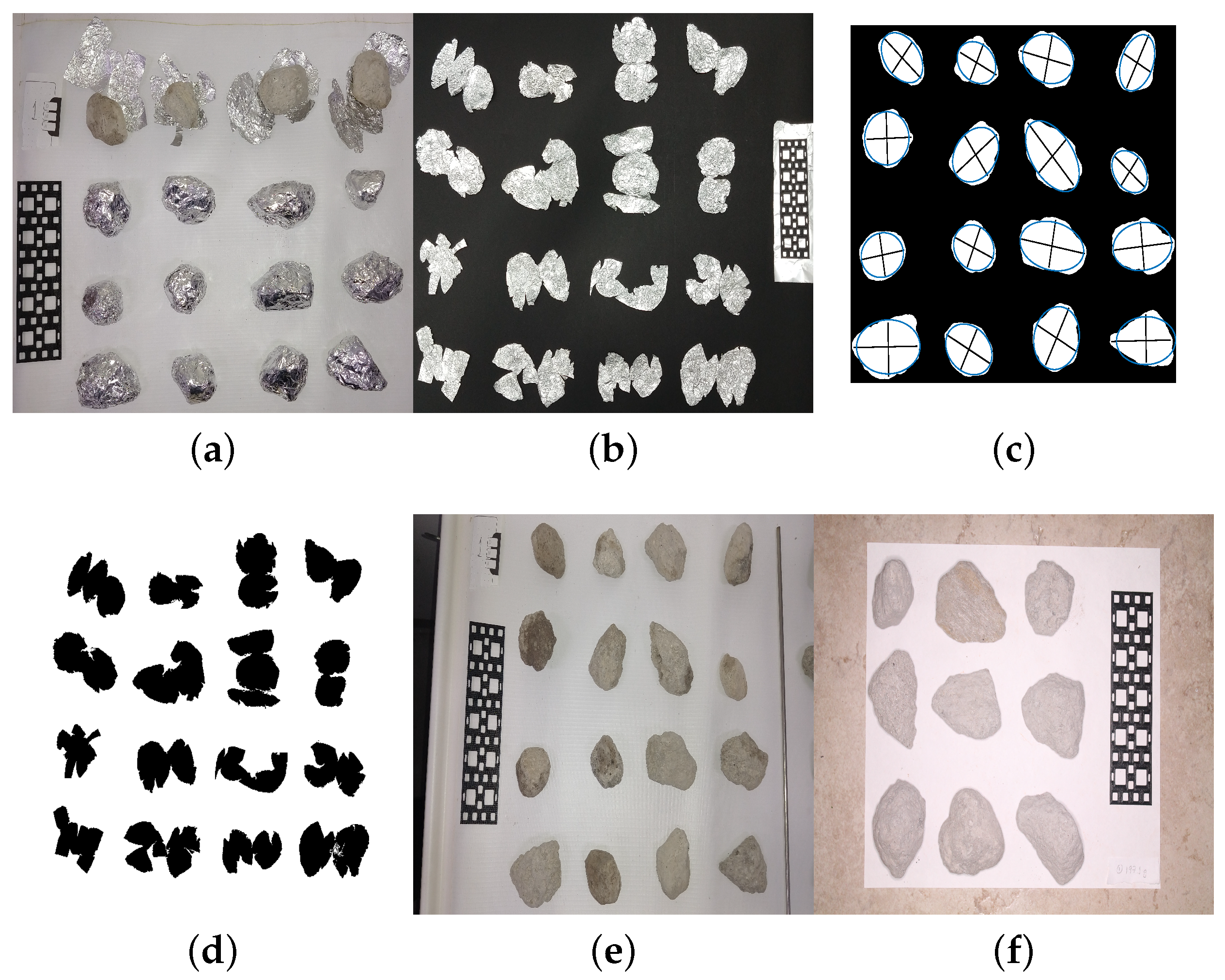
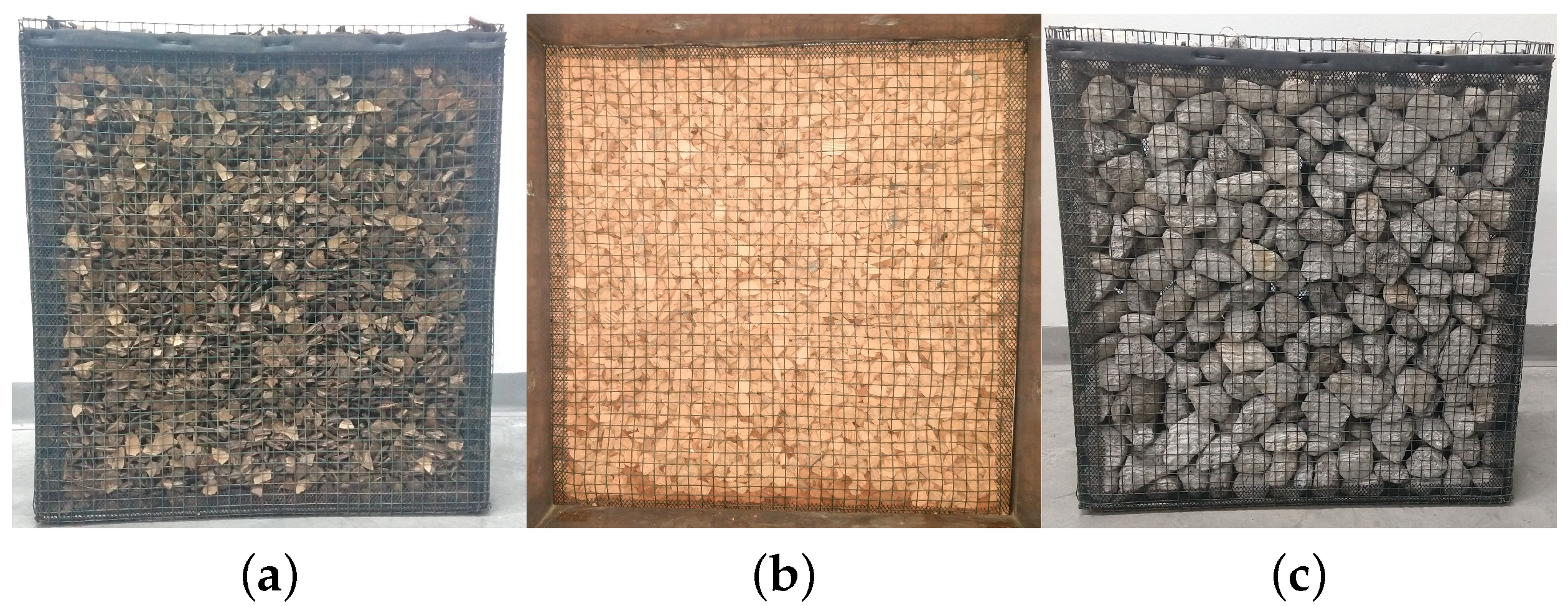
Three alternative materials: crushed coconut shells ($CS$), crushed burnt clay hollow brick ($BC$) and pumice stone ($PS$), were selected as raw materials to manufacture evaporative cooling pads, according to their availability and low-cost in the subtropical country of Colombia. Their cooling efficiency was compared with the frequently used cellulose cooling pad ($CL$, Munters Brasil Industria e Comércio Ltda, Araucária, Brazil). Two particle range sizes of coconut shell: 7.93 to 12.7 mm ($C{S}_1$) and 12.7 to 19.0 mm ($C{S}_2$); one range size of burnt clay hollow bricks: 12.7 to 19.0 mm; and two range sizes of pumice stone: 34.9 to 45.0 mm ($P{S}_1$) and 45.0 to 55.5 mm ($P{S}_2$), were evaluated. For each material, a pad of 0.5 m of height by 0.5 m of width was manufactured. All the cooling pads had a thickness of 0.1 m (Figure 1). The thickness was selected from a balance between pressure drop and cooling efficiency from previous research [28]. The pads were tested in an instrumented wind tunnel [32], increasing the air inlet velocity (u) from 0.5 m s${}^{-1}$ to 3.5 m s${}^{-1}$ for the cellulose pad or with the pressure below 160 Pa or until test failure due to water force out of the pad. In addition, three water flows (Q) around the recommended value of 6.2 L min${}^{-1}$ m${}^{-1}$ [46] were tested: 2, 6.2 and 10 L min${}^{-1}$ m${}^{-1}$, to determine their incidence over the pressure drop across the pad.

The mathematical model that described the fluid-dynamic and hygrothermal behaviour of cooling pads, proposed by Obando et al. [32], was used in order to compare the behaviour of the pads at different inlet air velocities (u: 0.5 to 2 m${}^{-1}$), thickness of pad (L: 0.05 to 0.15 m) and environmental conditions: dry-bulb temperature ($T_{d{b}_i}$: 25 to $35{}^{°}\mathrm{C}$) and relative humidity (${\varphi }_i$: 30 to 70%) of the inlet air. Twenty-one equidistant values from the inlet air relative humidity (${\varphi }_i$) interval and 11 values for each one of the other variables were selected, obtaining 307,461 combinations of different conditions to simulate for each pad. The cooling efficiency ($\eta$, Equation (1) [46], where $T_{d{b}_o}$ is the air temperature of the outlet air and $T_{w{b}_i}$ is the wet-bulb temperature of the inlet air), the THI (Equation (2) [45,47]), the change in the dry-bulb temperature ($\mathsf{\Delta }{T}_{db}$) and relative humidity ($\mathsf{\Delta }\varphi$) across the pads were compared. For this purpose, it was required to quantify the specific surface area ($\zeta$) and the convective heat ($h_H$) and mass ($h_M$) transfer coefficients of each pad.

$$\eta =\frac{T_{d{b}_i}-T_{d{b}_o}}{T_{d{b}_i}-T_{w{b}_i}}$$

(1)

$$THI=0.8T_{d{b}_o}+\frac{{\varphi }_o}{100}(T_{d{b}_o}-14.3)+46.3.$$

(2)

A specific surface area of 372.6 m${}^{-1}$ for the cellulose pad was considered [32]. For the other pads, it was estimated from the geometry of the particles. For the coconut shells and burn clay bricks, it was estimated from processing photographs of the particles, taking advantage of the fact that they present a planar geometry. The pumice stones were approximated to ellipsoids and the surface area was computed using the Knud Thomsen Formulae (A1) and the Dall Equation (A2) [48]. The results obtained with each expression were validated, covering the surface of each stone of a sample of 1000 g with one layer of aluminium foil. To determine the surface area of the aluminium foil, imaging processing was also employed. In Appendix A, the methodology followed is described in detail.

The convective heat and mass transfer coefficients were compute using the correlation of Hilper, modified for cooling pads [13] (Equation (3)).

$$Nu=a_1{\left(\frac{le}{L}\right)}^{b_1}R{e}^{c_1}P{r}^{0.37},$$

(3a)

$$Sh=a_2{\left(\frac{le}{L}\right)}^{b_2}R{e}^{c_2}S{c}^{0.37},$$

(3b)

where Nu, Re Pr, Sc and Sh were Nusselt, Reynolds, Prantl, Schmidt and Sherwood dimensional numbers, respectively [34]; $l_e$ is the specific length, computed as the inverse of $\zeta$, and L is the thickness of the cooling pad. The a’s, b’s and c’s parameters were fitted using the inlet and outlet air thermal conditions obtained from the experimental test in the wind tunnel for each pad. The convective heat and mass transfer coefficients were then computed using the $Nu$ and $Sh$ definitions as $h_H=Nu\times k\times l_e^{-1}$ and $h_M=Sh\times D_{AB}\times l_e^{-1}$ [34], with k as the thermal conductivity and $D_{AB}$ as the mass diffusion coefficient. A Wilcoxon rank sum statistical test (ranksum function, The MathWorks Inc. (Natick, MA, USA), MATLAB 2018a) [49,50,51] was used to validate the agreement between the experimental data and the predicted thermal conditions of the modelled air outlet. The coefficient of determination ($R^2$)), the Root Mean Square Error (RMSE) and regression plots of the dry-bulb temperature and relative humidity of the outlet air were also computed.

A porous medium such as the cooling pad is also characterized by its porosity and permeability. Porosity or void fraction ($\epsilon$) is a measure of the empty spaces between material particles. To determine the porosity of each material, a container of known volume was filled with the material and then water was added to the top of the container. The porosity was then computed using Equation (4). For hygroscopic materials, such as the pumice stone and burnt clay, the recipient was refilled after one hour of test. A porosity of 91.2% was considered for the cellulose pad [36,52].

$$\epsilon =\frac{\mathrm{Water}\mathrm{added}}{\mathrm{Container}\mathrm{volume}}.$$

(4)

The permeability (K) is an indication of the ability of the air to flow through a porous medium such as the pad. Several expressions had been proposed to relate it to the pressure drop ($\mathsf{\Delta }P$) across it and to the air velocity (u) [36,44]. The Darcy–Forchheimer Equation (5) shows a good description of the dynamics of the fluid across the porous medium [53], where $\beta$ is known as the Forchheimer coefficient.

$$-\frac{\mathsf{\Delta }P}{L}=\frac{\mu }{K}u+\rho \beta u^2.$$

(5)

To fit Equation (5) to the experimental data, the Least Absolute Residuals (LAR) method from the curve fitting toolbox of MATLAB^® was used [54].

3. Results

Table 3. Statistical descriptions of the inlet air dry-bulb temperature ($T_{d{b}_i}$) and relative humidity (${\varphi }_i$) for the wind tunnel tests. ${\overline{T}}_{d{b}_i}$ and ${\overline{\varphi }}_i$ are the means, ${\tilde{T}}_{d{b}_i}$ and ${\tilde{\varphi }}_i$ are the medians, $\sigma$ is the standard deviation and ${\sigma }^2$ is the variance.

Pad	Temperature				Relative Humidity
	${\overline{\mathit{T}}}_{{\mathit{db}}_{\mathit{i}}}$	${\tilde{\mathit{T}}}_{{\mathit{db}}_{\mathit{i}}}$	$\mathbf{\sigma }$	${\mathbf{\sigma }}^{\mathbf{2}}$	${\overline{\mathbf{\varphi }}}_{\mathit{i}}$	${\tilde{\mathbf{\varphi }}}_{\mathit{i}}$	$\mathbf{\sigma }$	${\mathbf{\sigma }}^{\mathbf{2}}$
	[${}^{°}$C]	[${}^{°}$C]	[${}^{°}$C]	[${}^{°}$C${}^{\mathbf{2}}$]	[%]	[%]	[%]	[%${}^{\mathbf{2}}$]
$CL$	24.6	24.6	0.5	0.3	62.1	62.5	4.1	16.4
$C{S}_1$	26.2	26.4	0.9	0.8	46.5	47.6	7.9	61.6
$C{S}_2$	25.4	25.4	0.2	0.1	46.0	46.0	1.3	1.8
$BC$	25.7	25.7	0.3	0.1	41.7	41.5	1.5	2.3
$P{S}_1$	26.9	26.9	0.4	0.2	41.0	41.0	5.3	28.2
$P{S}_2$	27.1	27.0	0.5	0.3	48.5	48.7	2.4	5.9

summarized the statistical description of the environmental conditions of the inlet air for each pad tested. These presented small changes during the test (below that $0.9{}^{°}\mathrm{C}$ and 7.9%), according to the standard deviation values. The alternative pads were tested in similar dry-bulb temperatures of the inlet air ($T_{d{b}_i}$) with mean values between 25.4 and 27.1 ${}^{°}$C and relative humidity (${\varphi }_i$) between 41.0 and 48.7%. $T_{d{b}_i}$ and ${\varphi }_i$ presented their maximum and minimum values during the cellulose pad tests, respectively.

Statistical description of the $\eta$ and THI of the outlet air are summarized in

Table 4. Statistical descriptions of the cooling efficiency ($\eta$) and the Temperature–Humidity Index (THI) for the wind tunnel tests. $\overline{\eta }$ and $\overline{\mathrm{THI}}$ are the means, $\tilde{\eta }$ and $\widetilde{\mathrm{THI}}$ are the medians, $\sigma$ is the standard deviation and ${\sigma }^2$ is the variance.

Pad	$\mathit{\eta }$				THI
	$\overline{\mathit{\eta }}$ [%]	$\tilde{\mathit{\eta }}$ [%]	$\mathit{\sigma }$ [%]	${\mathit{\sigma }}^2$ [%${}^2$]	$\overline{\mathbf{THI}}$	$\widetilde{\mathbf{THI}}$	$\mathit{\sigma }$	${\mathit{\sigma }}^2$
$CL$	68.6	68.8	6.0	35.6	68.8	68.8	0.4	0.2
$C{S}_1$	45.9	45.9	6.7	45.1	70.6	70.4	1.6	2.6
$C{S}_2$	65.1	65.0	1.8	3.3	67.6	67.60	0.2	0.1
$BC$	56.4	56.6	1.7	2.9	67.9	68.0	0.2	0.1
$P{S}_1$	45.2	45.4	1.9	3.6	70.4	70.1	0.8	0.6
$P{S}_2$	42.4	41.0	4.0	15.8	72.3	72.4	0.5	0.2

. Although the cellulose pad cooling was tested in low $T_{d{b}_i}$ and high ${\varphi }_i$, it presented the highest average cooling efficiency, followed by the $C{S}_2$ pad. The $C{S}_1$, $P{S}_1$ and $P{S}_2$ pads presented the lowest cooling efficiency considering that they were tested in the highest $T_{d{b}_i}$ and lowest ${\varphi }_i$. The lowest average THI value was for the $C{S}_2$ and $BC$ pads. The efficiency of the $CL$ pad was slightly above, because it was tested with higher ${\varphi }_i$ conditions. Through all experimental tests, ${\varphi }_i$ had a dispersion up to 7.9%, being significantly lower for $C{S}_2$, $BC$ and $P{S}_1$ pads. The dispersion of THI was up to 1.6 units for the $C{S}_1$ pad and significantly lower for the other pads.

Table 5. Statistical descriptions of the change in the dry-bulb temperature ($\mathsf{\Delta }T$) and relative humidity ($\mathsf{\Delta }\varphi$) across the pads in the wind tunnel tests. $\overline{\mathsf{\Delta }T}$ and $\overline{\mathsf{\Delta }\varphi }$ are the means, $\widetilde{\mathsf{\Delta }T}$ and $\widetilde{\mathsf{\Delta }\varphi }$ are the medians, $\sigma$ is the standard deviation and ${\sigma }^2$ is the variance.

Pad	$\mathsf{\Delta }\mathit{T}$				$\mathsf{\Delta }\mathit{\varphi }$
	$\overline{\mathsf{\Delta }\mathit{T}}$	$\widetilde{\mathsf{\Delta }\mathit{T}}$	$\mathbf{\sigma }$	${\mathbf{\sigma }}^{\mathbf{2}}$	$\overline{\mathsf{\Delta }\mathbf{\varphi }}$	$\widetilde{\mathsf{\Delta }\mathbf{\varphi }}$	$\mathbf{\sigma }$	${\mathbf{\sigma }}^{\mathbf{2}}$
	[${}^{°}$C]	[${}^{°}$C]	[${}^{°}$C]	[${}^{°}$C${}^{\mathbf{2}}$]	[%]	[%]	[%]	[%${}^{\mathbf{2}}$]
$CL$	−3.6	−3.6	0.7	0.4	21.2	21.1	3.7	13.7
$C{S}_1$	−3.6	−3.3	1.0	1.1	27.9	27.0	3.6	13.3
$C{S}_2$	−5.0	−5.0	0.2	0.1	35.2	35.3	1.4	1.9
$BC$	−4.8	−4.7	0.2	0.1	32.2	32.0	1.1	1.2
$P{S}_1$	−4.0	−4.0	0.5	0.2	25.5	25.5	2.3	5.1
$P{S}_2$	−3.2	−3.1	0.4	0.1	22.9	22.8	1.3	1.6

summarizes the statistical description of the change in the dry-bulb temperature ($\mathsf{\Delta }T=T_{d{b}_i}-T_{d{b}_o}$) and relative humidity ($\mathsf{\Delta }\varphi ={\varphi }_i-{\varphi }_o$) of the air across the pads. The mean and median of $\mathsf{\Delta }T$ follow the same behaviour of the ${\varphi }_i$, with the highest value for the $C{S}_2$ and $BC$ pads. These also present the highest $\mathsf{\Delta }\varphi$. The lowest $\mathsf{\Delta }\varphi$ was obtained for the $CL$ pad. In general, the average dry-bulb temperature drop was up to $5.0{}^{°}\mathrm{C}$ with a standard deviation of $\pm 1{}^{°}\mathrm{C}$ and the increment in ${\varphi }_i$ was between 21.2% and 35.5% with a standard deviation of $\pm 3.7\%$.

Statistical descriptions of the water temperature entering and leaving the cooling pads are shown in

Table 6. Statistical analysis of the water temperature ($T_w$) entering (i) and leaving (o) the pad in the wind tunnel tests. The difference between the inlet air wet-bulb temperature ($T_{w{b}_i}$) and the water temperature leaving the pad ($\mathsf{\Delta }{T}_w=T_{w{b}_i}-T_{w_o}$) is also shown. $\overline{T}$ is the mean [${}^{°}$C], $\tilde{T}$ is the median [${}^{°}$C], $\sigma$ is the standard deviation [${}^{°}$C] and ${\sigma }^2$ is the variance [${}^{°}$C${}^2$].

Pad	Entering				Leaving				$\mathsf{\Delta }{\mathit{T}}_{\mathit{w}}={\mathit{T}}_{{\mathit{wb}}_{\mathit{i}}}-{\mathit{T}}_{{\mathit{w}}_{\mathit{o}}}$
	${\overline{\mathit{T}}}_{{\mathit{w}}_{\mathit{i}}}$	${\tilde{\mathit{T}}}_{{\mathit{w}}_{\mathit{i}}}$	$\mathbf{\sigma }$	${\mathbf{\sigma }}^{\mathbf{2}}$	${\overline{\mathit{T}}}_{{\mathit{w}}_{\mathit{o}}}$	${\tilde{\mathit{T}}}_{{\mathit{w}}_{\mathit{o}}}$	$\mathbf{\sigma }$	${\mathbf{\sigma }}^{\mathbf{2}}$	${\overline{\mathsf{\Delta }\mathit{T}}}_{\mathit{w}}$	${\widetilde{\mathsf{\Delta }\mathit{T}}}_{\mathit{w}}$	$\mathbf{\sigma }$	${\mathbf{\sigma }}^{\mathbf{2}}$
$CL$	20.9	20.3	1.1	1.2	19.2	19.2	0.3	0.1	0.24	0.27	0.29	0.09
$C{S}_1$	21.7	20.8	1.5	2.2	18.7	18.4	1.4	1.9	−0.24	0.18	0.72	0.09
$C{S}_2$	19.9	19.3	1.7	3.0	17.1	17.0	0.3	0.1	0.59	0.73	0.33	0.11
$BC$	18.5	18.0	1.4	1.8	16.3	16.3	0.2	0.5	0.91	0.91	0.22	0.05
$P{S}_1$	20.3	20.2	1.3	1.7	17.8	17.6	0.9	0.8	0.31	0.50	0.58	0.34
$P{S}_2$	21.1	21.0	0.8	0.6	19.2	19.1	0.5	0.3	0.31	0.31	0.56	0.32

. The water that entered the pad had an average temperature below $21.1{}^{°}\mathrm{C}$, with a high variability ($1.7{}^{°}\mathrm{C}$). The differences between the temperature of the water when entering and leaving the pad were caused by the pump heating. This was more noticeable when low water flows were used in the tests. This also explains the high variability of the water temperature entering the pad. Temperatures of the water leaving the pad were closer and even lower than the inlet air wet-bulb temperature, as was expected from the adiabatic cooling process existing through the wetted pads.

The statistics analysis of the inlet air velocities, which were used in the wind tunnel to test the pads, are summarized in

Table 7. Statistics of inlet air velocity for the wind tunnel tests. $\overline{u}$ is the mean [m s${}^{-1}$], $\tilde{u}$ is the median [m s${}^{-1}$], $\sigma$ is the standard deviation [m s${}^{-1}$] and ${\sigma }^2$ is the variance [m${}^2$ s${}^{-2}$].

Pad	Test	$\overline{\mathit{u}}$	$\tilde{\mathit{u}}$	$\mathit{\sigma }$	${\mathit{\sigma }}^2$
$CL$	$u_1$	0.554	0.570	0.041	0.002
	$u_2$	1.067	1.070	0.049	0.002
	$u_3$	1.534	1.530	0.042	0.002
	$u_4$	2.032	2.030	0.046	0.002
	$u_5$	2.534	2.540	0.053	0.003
	$u_6$	2.994	2.990	0.057	0.003
	$u_7$	3.537	3.530	0.068	0.005
$C{S}_1$	$u_1$	0.299	0.220	0.145	0.021
	$u_2$	0.888	0.840	0.091	0.008
$C{S}_2$	$u_1$	0.503	0.500	0.030	0.001
	$u_2$	1.046	1.050	0.068	0.005
	$u_3$	1.398	1.410	0.059	0.004
$BC$	$u_1$	0.472	0.470	0.034	0.001
	$u_2$	0.969	0.970	0.049	0.002
$P{S}_1$	$u_1$	0.507	0.510	0.030	0.001
	$u_2$	1.015	1.010	0.056	0.003
	$u_3$	1.496	1.500	0.050	0.002
$P{S}_2$	$u_1$	0.521	0.520	0.042	0.002
	$u_2$	1.002	1.000	0.048	0.002
	$u_3$	1.490	1.490	0.047	0.002

. The cellulose pad allowed us to evaluate its behaviour for a wider range of velocities (0.5 to 3.5 m s${}^{-1}$). However, the alternative materials, except the $C{S}_1$ and $BC$ pads, were tested for three inlet air velocities; 0.5, 1.0 and 1.5 m s${}^{-1}$. The $C{S}_1$ and $BC$ pads were tested for two velocities, 0.5 and 1.0 m s${}^{-1}$, due to the higher pressure drop across the pads that caused water to come out of them. Small variations of the inlet air velocity through all the tests were presented. The average inlet air velocities for all the tests were similar.

The porosity ($\epsilon$) of the alternative pads varied between 0.44 and 0.59, which is considerably below that of the cellulose pad, which has an estimated value of 0.94. The lowest value was found for the $BC$ pad (0.44), followed by $C{S}_1$ and $P{S}_1$ pads, both with a porosity of 0.53. The $P{S}_2$ pad had a porosity of 0.56 and the $C{S}_2$ pad had the highest porosity (0.59).

The specific surface area ($\zeta$) was computed using the surface area per mass factor (m${}^2$ kg${}^{-1}$), which was obtained according to the methodology presented in Appendix A. The highest specific surface area was obtained for $C{S}_1$ (374.7 m${}^{-1}$–0.62 m${}^2$ kg${}^{-1}$), similar to that for $CL$ (372.6 m${}^{-1}$). The $BC$ material had a value (338.8 m${}^{-1}$–0.34 m${}^2$ kg${}^{-1}$) higher than that of the $C{S}_2$ material (304.7 m${}^{-1}$–0.56 m${}^2$ kg${}^{-1}$); although both materials had the same particle size, the $BC$ had thicker particles. For the $PS$ materials, their values were much lower: 137.6 m${}^{-1}$ (0.36 m${}^2$ kg${}^{-1}$) and 107.4 m${}^{-1}$ (0.30 m${}^2$ kg${}^{-1}$) for $P{S}_1$ and $P{S}_2$, respectively.

Table 8. Coefficients of correlation (3) used to compute the convective heat and mass transfer coefficients.

Pad	Correlation Coefficients						RMSE
	${\mathit{a}}_1$	${\mathit{b}}_1$	${\mathit{c}}_1$	${\mathit{a}}_2$	${\mathit{b}}_2$	${\mathit{c}}_2$	T [${}^{°}$C]	$\mathit{\varphi }$ [%]
$CL$	1.042	0.426	0.617	0.385	0.513	0.647	0.01	0.4
$C{S}_1$	0.093	0.935	1.300	0.727	0.589	0.748	0.02	0.7
$C{S}_2$	0.159	0.610	1.032	0.907	0.530	0.713	0.03	0.3
$BC$	0.196	0.700	0.998	0.554	0.629	0.809	0.03	0.3
$P{S}_1$	0.237	0.630	0.927	0.754	0.580	0.779	0.02	0.4
$P{S}_2$	0.186	0.890	1.064	0.689	0.641	0.864	0.01	0.3

shows the coefficients of Equation (3) fitted to the experimental data using the specific surface area found for each pad, and the RMSE values computed between the experimental and the predicted values of the dry-bulb temperature and the relative humidity of the outlet air, which were obtained using the mathematical model proposed by Obando et al. [32].

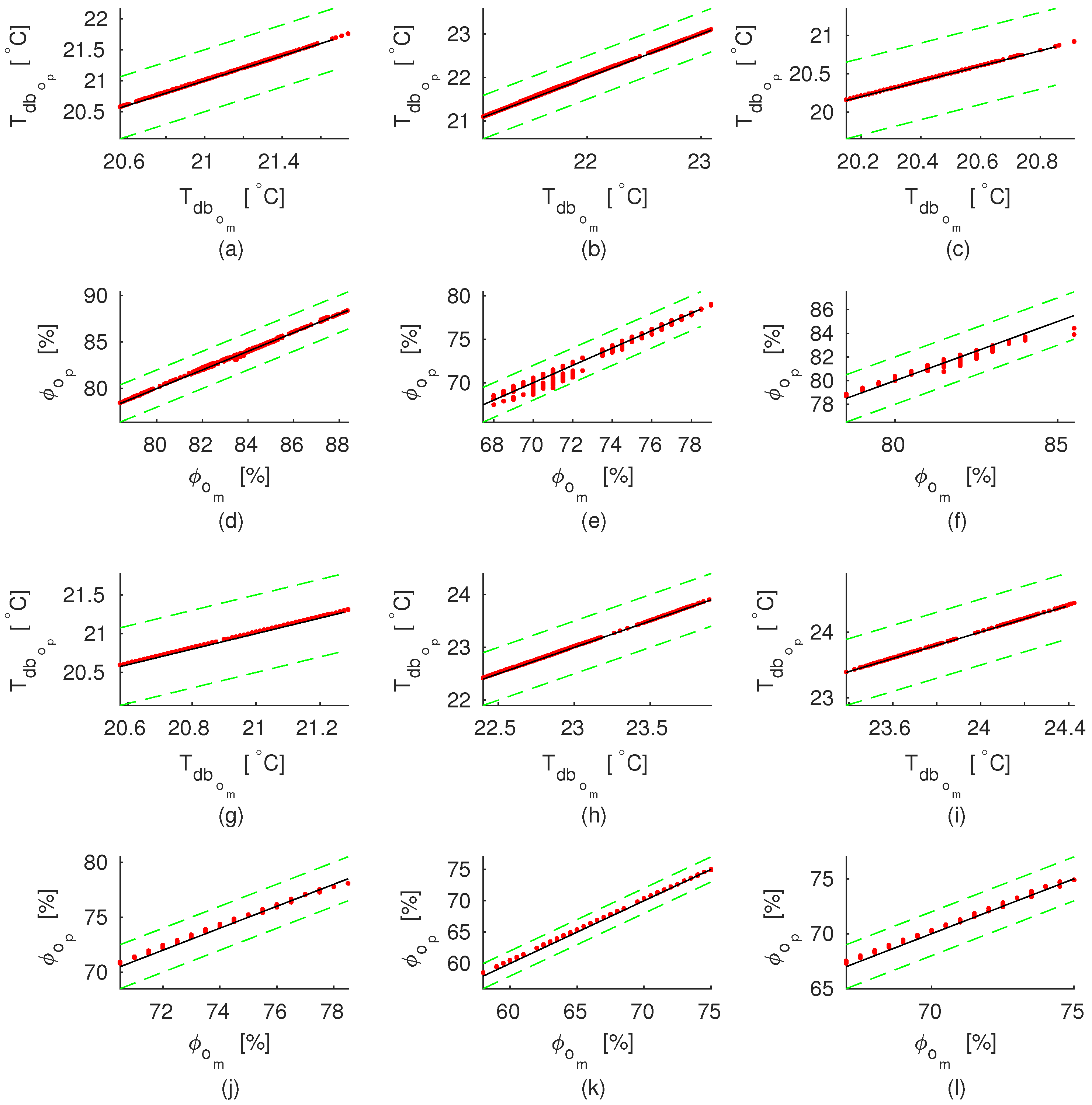
Figure 2 shows a comparison between the predictions obtained with the mathematical model and the experimental data. For all the pads, a linear relation around the equality line (black solid line) was presented. The Wilcoxon signed rank statistical test found no statistically significant difference between the predictions and the experimental data (p-value > 0.05). ${\varphi }_o$ was slightly overestimated for the alternative materials but with a bias deviation of less than 5% (dashed lines). Those results allow us to consider that the model is suitable for predicting the behaviour of the pads for other operative and constructive conditions.

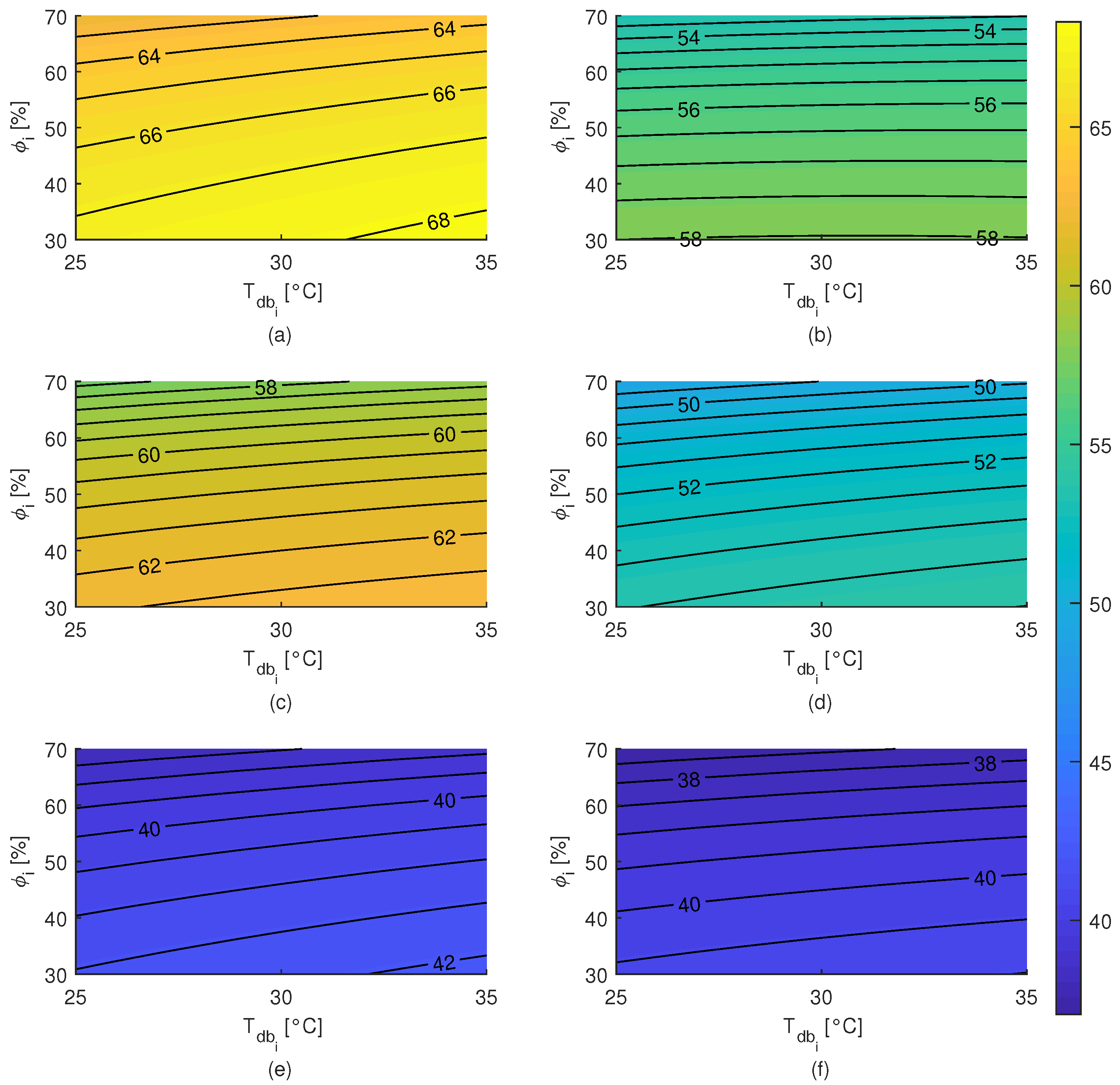
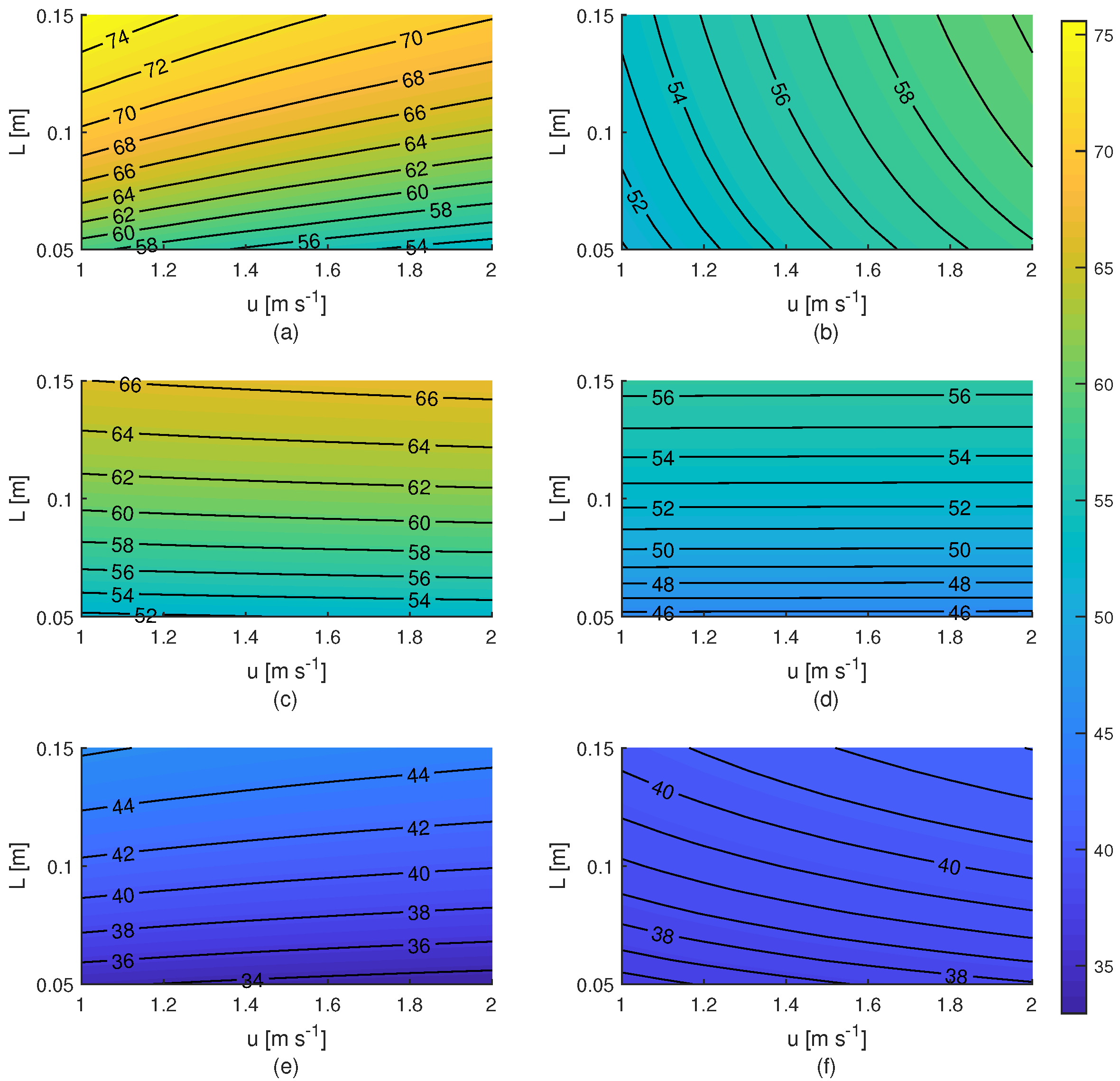
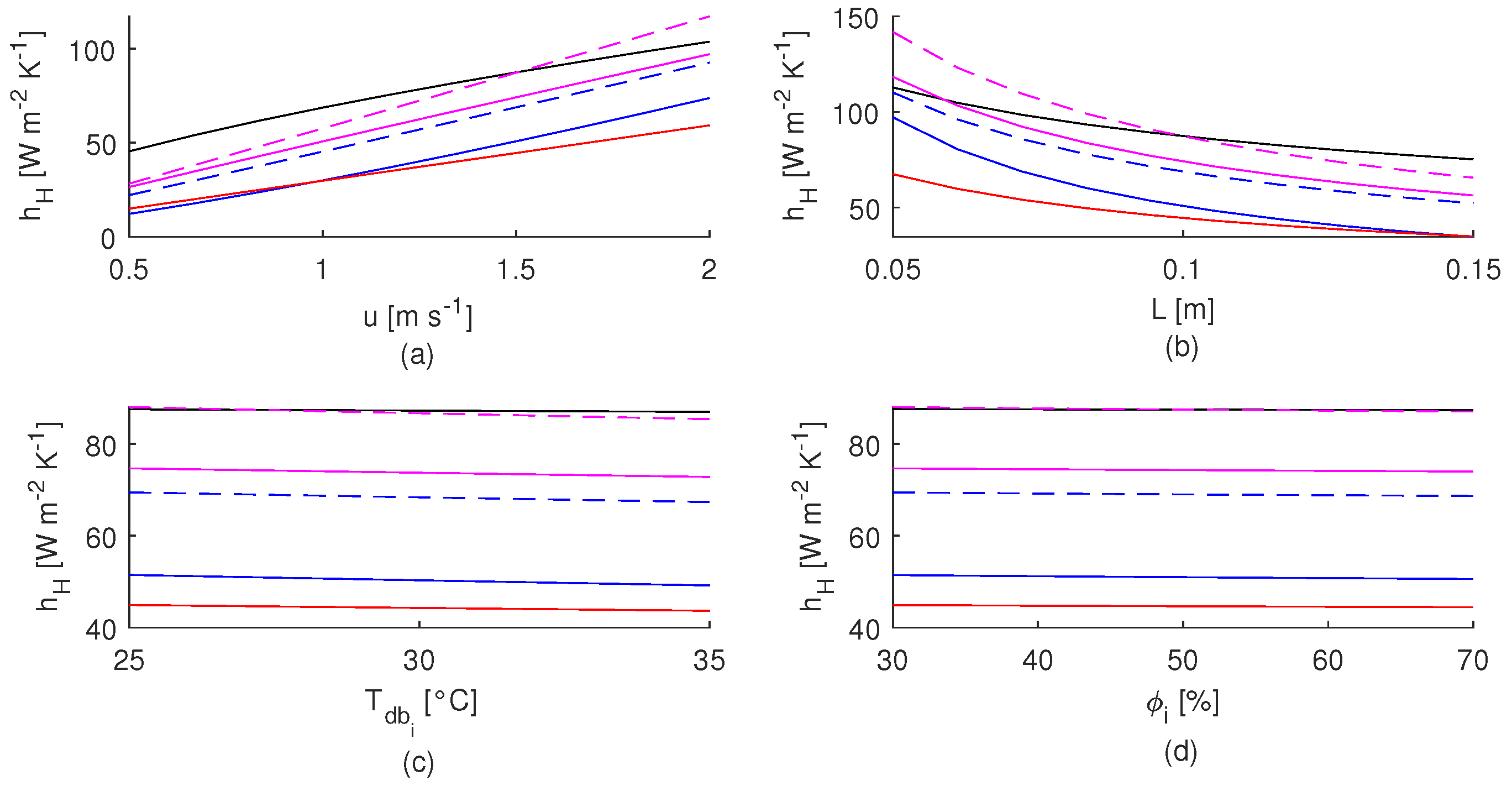
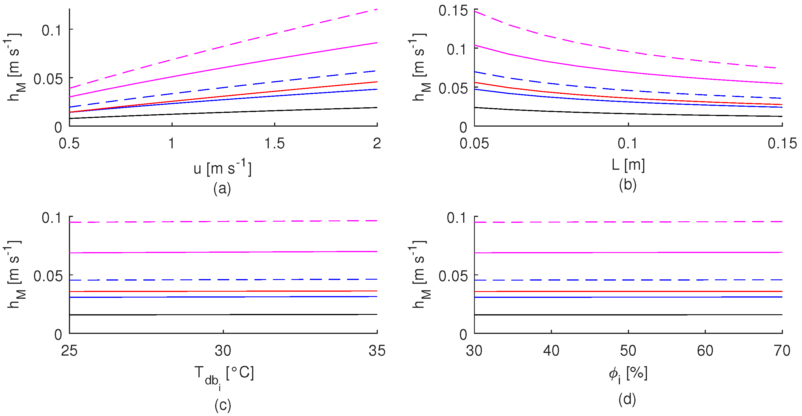
In Figure 3 and Figure 4, the behaviour of the convective heat and mass transfer coefficients as functions of operative and constructive variables, such as air velocity (u), pad thickness (L), dry-bulb temperature ($T_{d{b}_i}$) and relative humidity (${\varphi }_i$) of inlet air, are shown. For this matter, the other independent variables are considered constants (u = 1.5 m s${}^{-1}$, L = 0.1 m, $T_{d{b}_i}$ = 30 ${}^{°}$C, ${\varphi }_i$ = 60%).

The relationship between the convective heat transfer coefficient ($h_H$) and the inlet air velocity is shown in Figure 3a. A linear relationship between them is presented, corresponding to an increase in the flow of heat transferred between the air crossing the pad and the wetted pad surface when the inlet air velocity increasing. Figure 3b shows the relation between $h_H$ and the thickness of the pad; when L decreases, $h_H$ rises to compensate for the decrease in the wet surface area. Figure 3c,d shows that $h_H$ remains almost constant when the dry-bulb temperature and relative humidity of inlet air change. The effect of the inlet air velocity and pad thickness change were more relevant. With the exception of the $P{S}_2$ pad, $CL$ present the highest $h_H$ values.

The relationship between the convective mass transfer coefficient ($h_M$) and the inlet air velocity was shown in Figure 4a. An increase in $h_H$ due to increasing the air velocity is presented. Thus, the evaporation rate increases according to the inlet air velocity. Figure 4b shows the relationship between $h_M$ and the thickness of the pad. $h_H$ also increases when the thickness of the pad decreases, to compensate for the reduction of the wet surface area. Figure 3c,d shows that $h_M$ also remains almost constant when the dry-bulb temperature and relative humidity of inlet air change. The effect of the inlet air velocity and pad thickness changes was more significant than that caused by the dry-bulb temperature and relative humidity. In all the plots shown in Figure 4, $h_H$ is inversely proportional to the specific surface area of each material. $h_M$ had the lowest values for the $CS$ pad, indicating that the amount of water evaporating from this pad is less in comparison with the others.

The surface response of $\eta$, THI, $\mathsf{\Delta }T$ and $\mathsf{\Delta }HR$ as functions of each pair of input variables: $T_{d{b}_i}$-${\varphi }_i$ and u-L are shown in Figure A4, Figure A5, Figure A6, Figure A7, Figure A8, Figure A9, Figure A10 and Figure A11 in Appendix B. These data were obtained evaluating the model of each pad in the simulation points previously defined.

In order to simultaneously compare all the pads, an average operating condition was analysed: u = 1.5 m s${}^{-1}$, $L=0.1$ m, $T_{d{b}_i}$ = 30 ${}^{°}$C and ${\varphi }_i$ = 60%. For this, one variable at a time was changed in the simulation region and each output variable was plotted separately. A detailed analysis of the behaviour of the cooling pads is presented in the following sections.

3.1. Cooling Efficiency

In Figure 5, the variation of the cooling efficiency with respect to air velocity, pad thickness, dry-bulb temperature and relative humidity of the inlet air for each pad analysed is shown. The $CL$ pad shows the highest cooling efficiency, followed by the $CS$ pads. The $PS$ pads presented the lowest one. An inversely proportional correlation between the cooling efficiency and inlet air velocity for $CL$ and $P{S}_1$ pads is shown in the Figure 5a, meanwhile a direct proportional correlation is presented for the other ones. The effect of the inlet air velocity over the cooling efficiency for the $BC$ material was negligible. In the range of the inlet air velocity analysed, $CL$ and $C{S}_1$ pads presented the biggest change in the cooling efficiency, up to 5.8 and 7.0%, respectively. The change was below 1.5% for the other pads. Figure 5b shown that the effect of the pad thickness over the cooling efficiency was stronger, with up to 17.4% of change for the $CL$ pad. Figure 5c,d show the effect of the inlet air thermal conditions. All the pads show a similar behaviour, the cooling efficiency increase for high dry-bulb temperatures and low relative humidity of inlet air. The cooling efficiency was more susceptible to the changes in the relative humidity of the inlet air (${\varphi }_i$) in comparison with the changes of the dry-bulb temperature of the inlet air ($T_{d{b}_i}$). For the conditions evaluated, the cooling efficiency increased up to 1.2% ($CL$ pad) when $T_{d{b}_i}$ increase, and fall up to 5.0% ($CL$ pad) when ${\varphi }_i$ augment.

No statistically significant evidence was found (p-value = 0.5114) to consider that there are differences between the medians of the $P{S}_1$ and $P{S}_2$ pads for the cooling efficiency and pad thickness relationship.

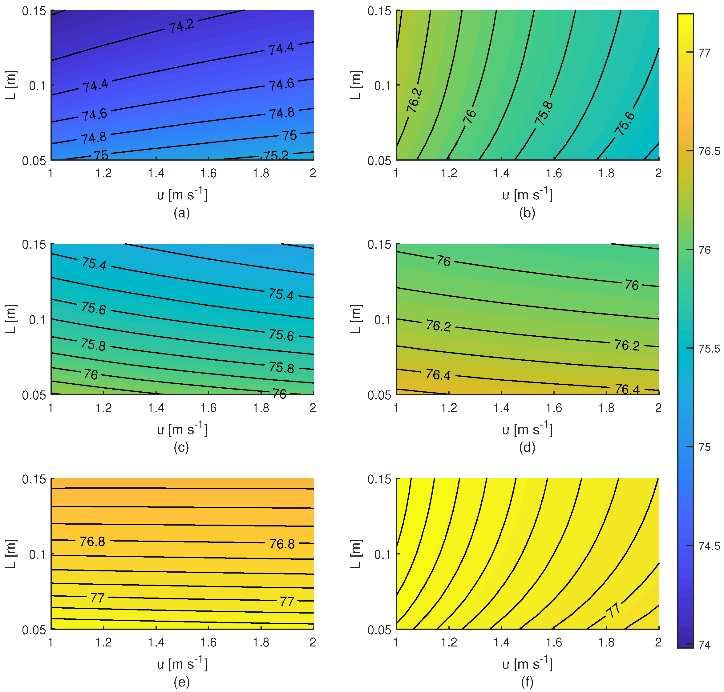
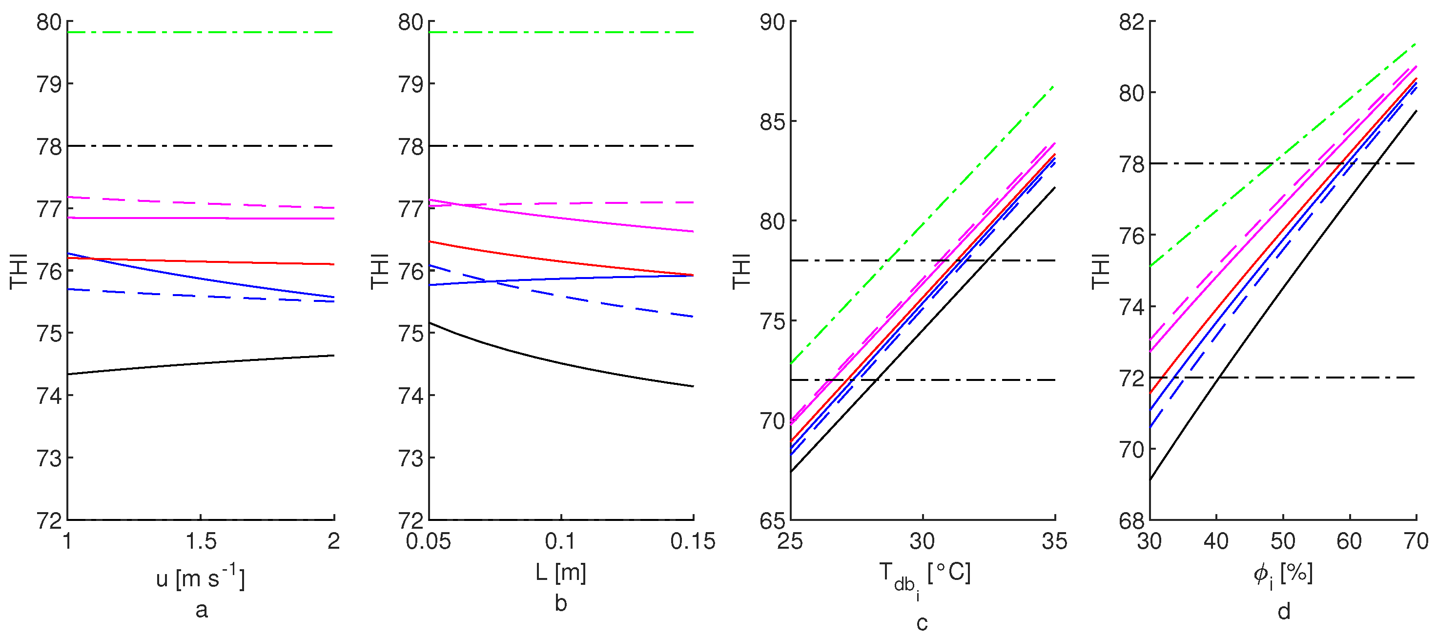
3.2. Temperature–Humidity Index

Figure 6 shows the behaviour of the Temperature–Humidity Index computed for the outlet pad thermal conditions. THI computed for the external thermal conditions was also shown for comparison purposes (green dash-doted line). THI at pads outlet was below the THI at pad inlet, thus all the pads improved the thermal comfort conditions of the air at outlet. As a reference, the zone of the middle thermal stress defined for cattle is shown with black dash-dot lines ($72\le THI\le 78$) [55]. For the inlet thermal conditions analysed ($T_{d{b}_i}=30{}^{°}\mathrm{C}$ and ${\varphi }_i$ = 60%), Figure 6a,b shows that the THI of the $CL$ pad was furthest away, around 5.5 units below the external THI, followed by the $CS$ pads (around 4.1 units below). The $PS$ pads were closer to the external THI (around 2.6 units below). The inlet air velocity and pad thickness changes have little effect over THI. Figure 6a shows that the THI behaviour of the $CL$ pad varied inversely to the alternative pads, which decrease THI when increasing the inlet air velocity. It is not possible to generalize the behaviour due to the pad thickness influence, because for the $C{S}_1$ and $P{S}_2$ pads it was opposite to the $CL$ pad’s behaviour, as is shown in Figure 6b. Due to the way THI was computed, the dry-bulb temperature and relative humidity of inlet air have a strong influence over it. When $T_{d{b}_i}$ changed, the THI upper limit of the middle comfort zone (THI = 78) in Figure 6c was reached before by the $P{S}_2$ pad at $30.7{}^{°}\mathrm{C}$ and $1.7{}^{°}\mathrm{C}$ above it by the $CL$ pad. THI increased linearly with $T_{d{b}_i}$ with the same slope for all the pads (≈1.4 THI units per $T_{d{b}_i}$ unit). A similar behaviour occurs when ${\varphi }_i$ changed. THI was less susceptible to ${\varphi }_i$ changes than to $T_{d{b}_i}$ ones (≈0.3 THI units per ${\varphi }_i$ unit for the $CL$ pad). The upper limit of the middle thermal comfort zone (THI = 78) is reached before by the $P{S}_2$ pad when ${\varphi }_i$ was 54.8% and later by the $CL$ pad when ${\varphi }_i$ was 63.9%.

Non statistically significant evidence was found (0.3246 ≤ p-value ≤ 0.7427) to consider that there are differences between the medians of all the pads for the THI and dry-bulb temperature of the inlet air relationship, between the medians of all the pads (except between $CL$ and $PS$ pads) for the THI and relative humidity of the inlet air relationship (0.1020 ≤ p-value ≤ 0.8014).

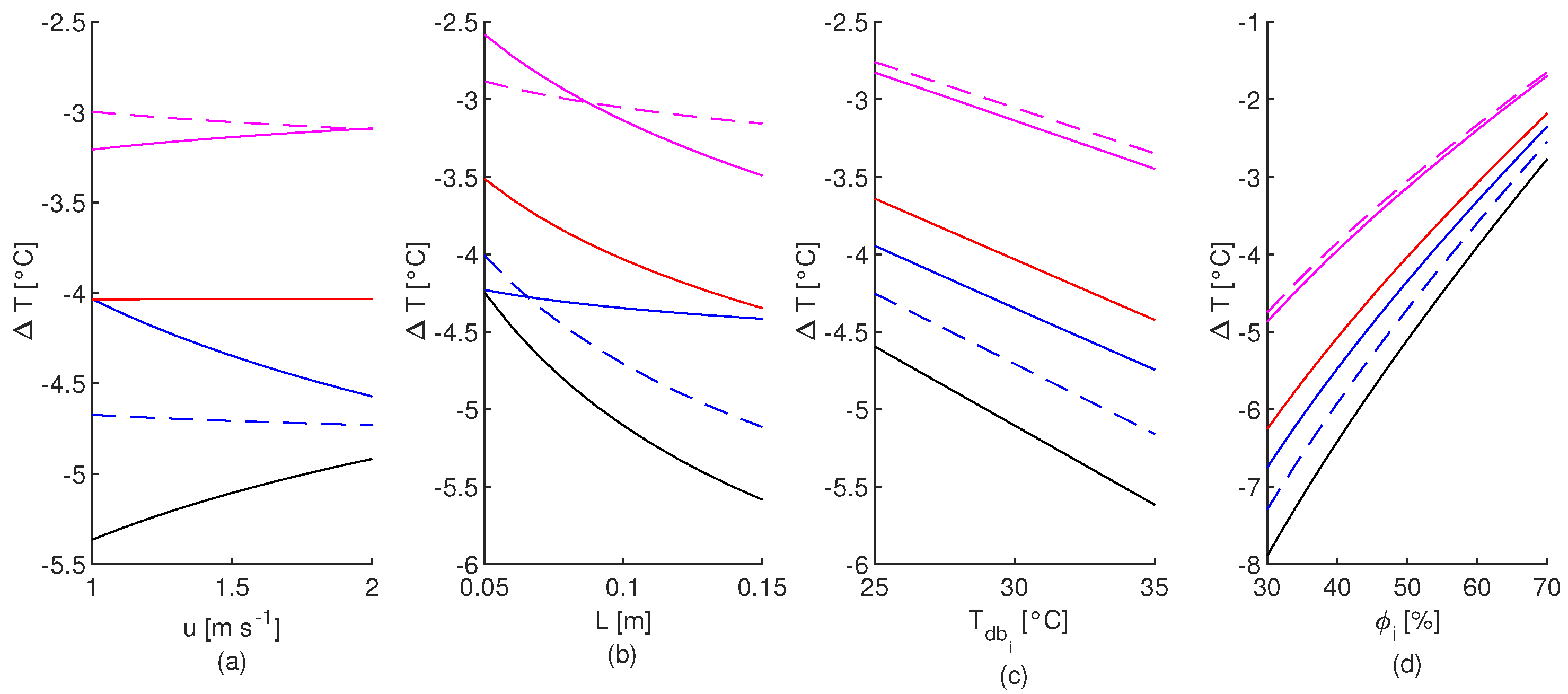
3.3. Air Dry-Bulb Temperature Drop

As is shown in Figure 7, $\mathsf{\Delta }T$ was highest for the $CL$ pad and lowest for the $PS$ pads. For low inlet air velocity $\mathsf{\Delta }T$ was highest for $CL$ and $C{S}_2$ pads, as is shown in Figure 7a. There is no generalized behaviour of $\mathsf{\Delta }T$ as a function of u, with $CL$ and $P{S}_1$ presented a direct correlation but inverse for the other pads. However, the influence of the inlet air velocity over $\mathsf{\Delta }T$ could be neglected since a change of 1 m s${}^{-1}$ increased $\mathsf{\Delta }T$ up to $0.5{}^{°}\mathrm{C}$ for the $C{S}_1$ pad; for the other pads $\mathsf{\Delta }T$ was lower. On the other hand, changes in the pad thickness (Figure 7b), dry-bulb temperature (Figure 7c) and relative humidity of the inlet air (Figure 7c) have a greater impact on $\mathsf{\Delta }T$. Increasing the thickness of the pad increases $\mathsf{\Delta }T$ in $1.3{}^{°}\mathrm{C}$ for the $CL$ pad; for the other pads $\mathsf{\Delta }T$ also increases in a lower range. $\mathsf{\Delta }T$ changed linearly with the dry-bulb temperature and relative humidity of the inlet air, being more susceptible to the changes of relative humidity. When $T_{d{b}_i}$ rises, $\mathsf{\Delta }T$ increases $1.0{}^{°}\mathrm{C}$ and $0.6{}^{°}\mathrm{C}$ for the $CL$ and $P{S}_2$ pads, respectively, which correspond to an increment of $0.1{}^{°}\mathrm{C}$ and $0.06{}^{°}\mathrm{C}$ per unit of $Ti$ change. When ${\varphi }_i$ increase, $\mathsf{\Delta }T$ decrease $5.1{}^{°}\mathrm{C}$ and $3.1{}^{°}\mathrm{C}$ for the $CL$ and $P{S}_2$ pads, respectively, that correspond to a decrease of $0.13{}^{°}\mathrm{C}$ and $0.08{}^{°}\mathrm{C}$ per unit of ${\varphi }_i$ change.

Non statistically significant evidence was found to consider that there are differences between the medians of $P{S}_1$ and $P{S}_2$ pads for the dry-bulb temperature drop relationship with the pad thickness (p-value = 0.5114) and inlet air dry-bulb temperature (p = 0.3246); between the medians of pads $CL-C{S}_1$, $CL-C{S}_2$, $CS-BC$, $C{S}_1-C{S}_2$ and $P{S}_1-P{S}_2$ for the dry-bulb temperature drop and relative humidity of the inlet air relationship (0.1249 ≤ p-value ≤ 0.8014).

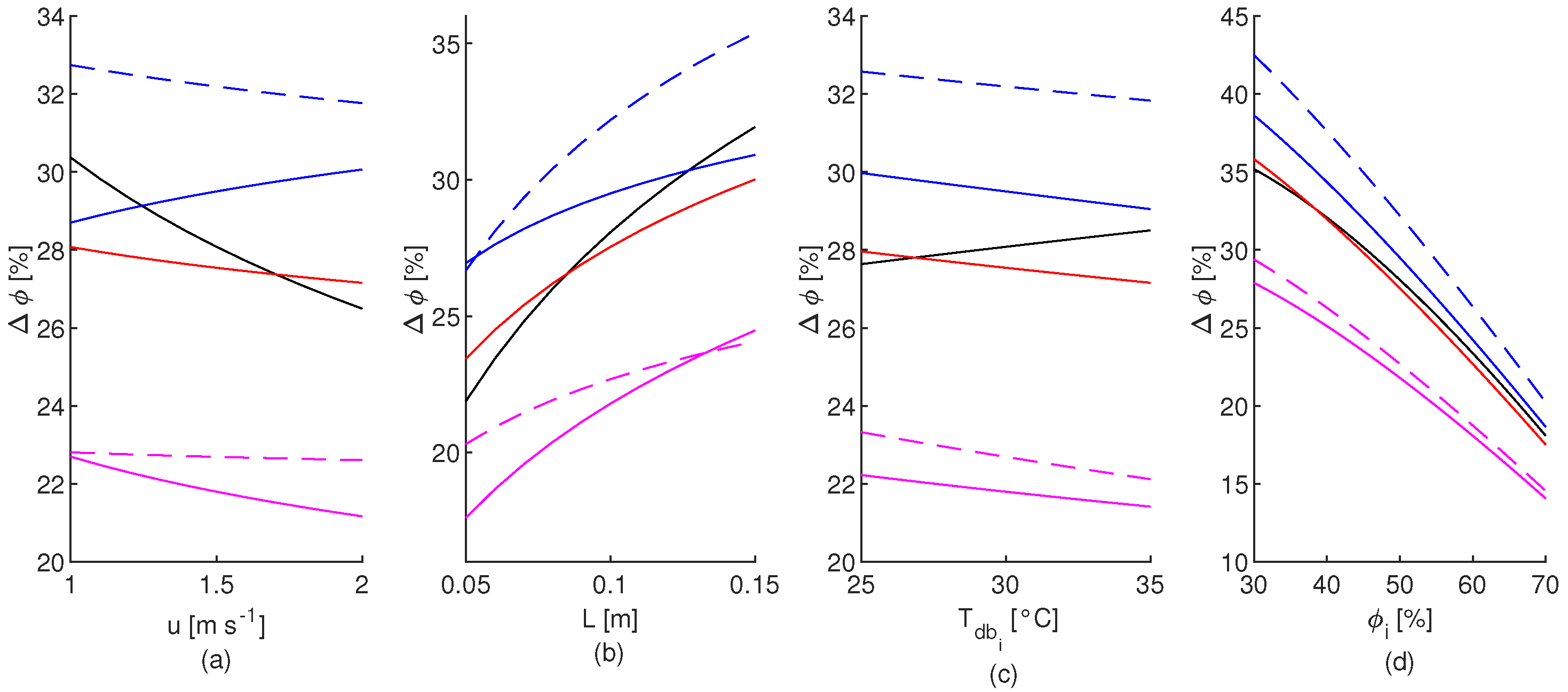
3.4. Relative Humidity Increase

Contrary to the results presented before, the increase of the relative humidity at the outlet of the pads ($\mathsf{\Delta }\varphi$) for the $CL$ pad was located between the alternative pad’s results, as is shown in Figure 8. The lowest $\mathsf{\Delta }\varphi$ was for the $PS$ pads, followed by the $CL$ pad, while the $C{S}_2$ had the highest. $\mathsf{\Delta }\varphi$ of the $C{S}_1$ pad increased when the inlet air velocity increasing; opposite to the behaviour of the other alternative pads (Figure 8a). The $CL$ pad presented the highest change of $\mathsf{\Delta }\varphi$ (3.8%) due to inlet air velocity. The influence of the pad thickness over $\mathsf{\Delta }\varphi$ is stronger, changing up to 10.0% for the $CL$ pad (Figure 8b). $\mathsf{\Delta }\varphi$ increases when increasing the pad thickness, for all the pads. Increasing the dry-bulb temperature of inlet air had a non-significant effect on $\mathsf{\Delta }\varphi$, with a maximum change of 1.2% for the $P{S}_2$ pad (Figure 8c). In this case, the behaviour of the $CL$ pad was opposite to the alternative pads, indicating that the $CL$ pad increase the evaporation rate when $T_{d{b}_i}$ increased. $\mathsf{\Delta }\varphi$ across the pads was more susceptible to the changes in the relative humidity of inlet air. Figure 8d shows that all the pads present the same behaviour, decreasing $\mathsf{\Delta }\varphi$ when increasing ${\varphi }_i$. The changes of $\mathsf{\Delta }\varphi$ were between 22.3% and 13.4% for the $C{S}_2$ and $P{S}_1$ pads, respectively. Those values correspond to a decrease of 0.6% and 0.3% per unit increment of ${\varphi }_i$, respectively. When ${\varphi }_i$ increased, decrease the ability of the air to hold the water vapour and consequently evaporate a less amount of water from the pads.

Non statistically significant evidence was found to consider that there are differences between the medians of $CL$ and $BC$ pads for the relative humidity increment and inlet air velocity relationship (p-value = 0.2934); between the medians of the paired pads $CL-C{S}_1$, $CL-BC$, $C{S}_1-C{S}_2$ and $P{S}_1-P{S}_2$ for the relative humidity increment and the pad thickness relationship (0.2934 ≤ p-value ≤ 0.6936); and between the medians of the pads $CL-C{S}_1$, $CL-BC$, $C{S}_1-C{S}_2$, $C{S}_1-BC$ and $P{S}_1-P{S}_2$ for the relative humidity increment and the relative humidity of inlet air relationship (0.2085 ≤ p-value ≤ 0.8999).

Table 9. Cooling efficiency ($\eta$), Temperature–Humidity Index (THI), dry-bulb temperature drop ($\mathsf{\Delta }T$) and relative humidity increment ($\mathsf{\Delta }\varphi$) for average input variables: inlet air velocity (u = 1.5 m s${}^{-1}$), pad thickness (L = 0.1 m), dry-bulb temperature ($T_{d{b}_i}$ = 30 ${}^{°}$C) and relative humidity of inlet air (${\varphi }_i$ = 50%). $\mathsf{\Delta }\eta$ is the difference between $\eta$ of the alternative pads and the $CL$ pad. $\mathsf{\Delta }THI$ is the difference between the THI compute with the outlet and inlet (79.8) air thermal conditions.

Pad	$\mathit{\eta }$ ($\mathsf{\Delta }\mathit{\eta }$) [%]	THI ($\mathsf{\Delta }\mathit{THI}$)	$\mathsf{\Delta }\mathit{T}$ [${}^{°}$C]	$\mathsf{\Delta }\mathit{\varphi }$ [%]
$CL$	66.3	74.5 (5.3)	−5.1	28.1
$C{S}_1$	56.4 (−9.9)	75.9 (3.9)	−4.3	29.5
$C{S}_2$	61.1 (−5.2)	75.6 (4.2)	−4.7	32.2
$BC$	52.4 (−13.9)	76.1 (3.7)	−4.0	27.5
$P{S}_1$	40.7 (−25.6)	76.8 (3.0)	−3.1	21.8
$P{S}_2$	39.6 (−26.7)	77.1 (2.7)	−3.0	22.7

shows a comparison between the output pad variables: $\eta$, THI, $\mathsf{\Delta }T$ and $\mathsf{\Delta }\varphi$ for constant input variables: u = 1.5 m s${}^{-1}$, L = $0.1$ m, $T_{d{b}_i}$ = 30 ${}^{°}$C and ${\varphi }_i$ = 50%. For this conditions, the $CS$ pads present the best behaviour between the alternative pads: highest cooling efficiency, lowest THI, highest dry-bulb temperature drop but also the highest relative air humidity increasing. The lowest $\mathsf{\Delta }T$ of the $PS$ pads do not compensate the increasing of $\varphi$, obtaining the highest values of THI.

3.5. Pressure Drop across the Pad

Table 10. Statistics of pressure drop across the cooling pad ($\mathsf{\Delta }P$) for the wind tunnel tests. $\overline{\mathsf{\Delta }P}$ is the mean [Pa], $\widetilde{\mathsf{\Delta }P}$ is the median [Pa], $\sigma$ is the standard deviation [Pa] and ${\sigma }^2$ is the variance [Pa${}^2$].

Pad	Test	$\overline{\mathsf{\Delta }\mathit{P}}$	$\widetilde{\mathsf{\Delta }\mathit{P}}$	$\mathit{\sigma }$	${\mathit{\sigma }}^2$
$CL$	$u_1$	1.2606	1.2700	0.0955	0.0091
	$u_2$	3.5558	3.6100	0.2227	0.0496
	$u_3$	6.9345	6.9500	0.2199	0.0484
	$u_4$	12.3764	12.3800	0.3067	0.0941
	$u_5$	18.2361	18.2700	0.4733	0.2240
	$u_6$	24.0571	24.2300	0.5083	0.2584
	$u_7$	31.5677	31.8500	0.9008	0.8114
$C{S}_1$	$u_1$	20.7298	10.5400	20.3817	415.4150
	$u_2$	109.3886	115.4700	22.1462	490.4554
$C{S}_2$	$u_1$	22.2006	21.0000	2.7782	7.7182
	$u_2$	89.9411	78.3650	19.5662	382.8370
	$u_3$	133.2440	132.3500	3.7064	13.7374
$BC$	$u_1$	33.6239	30.7100	8.5841	73.6868
	$u_2$	134.8465	131.6900	24.7958	614.8340
$P{S}_1$	$u_1$	17.6566	17.7000	1.2807	1.6401
	$u_2$	60.6392	61.8000	6.4748	41.9233
	$u_3$	116.5752	112.2400	7.9055	62.4964
$P{S}_2$	$u_1$	12.8821	12.7850	1.2633	1.5959
	$u_2$	40.8870	41.4500	2.7954	7.8142
	$u_3$	87.5552	88.1300	4.6572	21.6894

summarized the statistical description of the pressure drop measured across the pads ($\mathsf{\Delta }P$). Larger differences of the average values of $\mathsf{\Delta }P$ between the cellulose and the alternative pads were evident. Even at high speeds ($u_7\approx$ 3.5 m s${}^{-1}$), the cellulose $\mathsf{\Delta }P$ is around the obtained for the air velocity tested in the other materials (for $u\le 1$ m s${}^{-1}$). The variability of the measured $\mathsf{\Delta }P$ also shows big differences. This is mainly due to an increase in resistance to air flow caused by increasing water flow through the pads. For each air velocity, up to three water flows were evaluated. The low variability of the $C{S}_2$ material for the inlet air velocity $u_3$ was because, in this test, only the lowest flow of water was evaluated; when water flow was increased, liquid water came out of the pads. The $PS$ pads present the lowest variability from the alternative pads, indicating that water flow does not considerably affect the air flow resistance in them.

The average values of water flow presented in

Table 11. Statistics of water flow for all tests in the wind tunnel. $\overline{Q}$ is the mean [L min${}^{-1}$ m${}^{-1}$], $\tilde{Q}$ is the median [L min${}^{-1}$ m${}^{-1}$], $\sigma$ is the standard deviation [L min${}^{-1}$ m${}^{-1}$] and ${\sigma }^2$ is the variance [L${}^2$ min${}^{-2}$ m${}^{-2}$].

Pad	Test	$\overline{\mathit{Q}}$	$\tilde{\mathit{Q}}$	$\mathit{\sigma }$	${\mathit{\sigma }}^2$
$CL$	$Q_1$	1.9450	1.9400	0.0414	0.0017
	$Q_2$	6.1400	6.1200	0.0573	0.0033
	$Q_3$	10.0170	10.0400	0.0440	0.0019
$C{S}_1$	$Q_1$	1.9827	1.9400	0.0852	0.0073
	$Q_2$	6.1321	6.1200	0.1640	0.0269
	$Q_3$	8.1764	8.1300	0.4248	0.1805
$C{S}_2$	$Q_1$	1.9896	1.9800	0.1389	0.0193
	$Q_2$	5.9684	6.0400	0.2677	0.0716
	$Q_3$	9.7014	9.7600	0.5464	0.2986
$BC$	$Q_1$	2.0832	2.0500	0.2869	0.0823
	$Q_2$	6.0147	5.9800	0.2579	0.0665
	$Q_3$	9.7360	9.7900	0.4150	0.1723
$P{S}_1$	$Q_1$	2.3979	2.4400	0.2310	0.0534
	$Q_2$	6.0732	6.0800	0.7191	0.5171
	$Q_3$	8.6864	8.6600	0.6682	0.4465
$P{S}_2$	$Q_1$	2.1481	2.1600	0.2472	0.0611
	$Q_2$	6.3353	6.2200	0.6723	0.4520
	$Q_3$	8.6104	8.4800	0.6734	0.4535

were around 2, 6.2 and 10 L min${}^{-1}$ m${}^{-1}$ values as defined before. The variability of the water flow measurements was below 0.7 L min${}^{-1}$ m${}^{-1}$, being considerably lowest for the cellulose pad tests.

Average pressure drop across the cellulose pad varied from 1.2 Pa when u = 0.5 m s${}^{-1}$ and Q = 2 L min${}^{-1}$ m${}^{-1}$ to 32.3 Pa when u = 3.5 m s${}^{-1}$ and Q = 10 L min${}^{-1}$ m${}^{-1}$. While the pad with $P{S}_2$ material was above 10 Pa and the other ones were above 20 Pa for the minimum speed tested. This shows a big difference between $\mathsf{\Delta }P$ of the cellulose and the alternative materials. 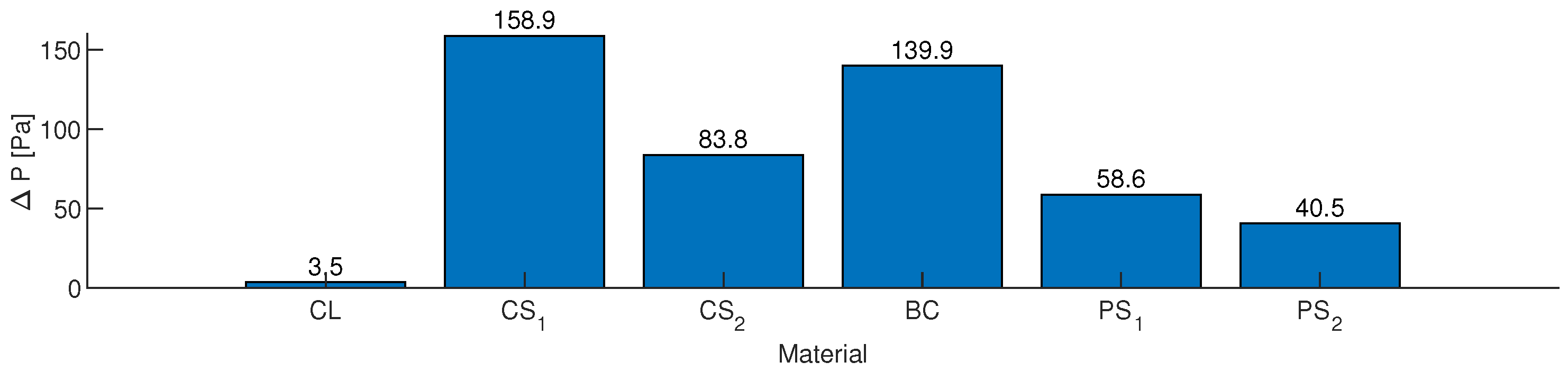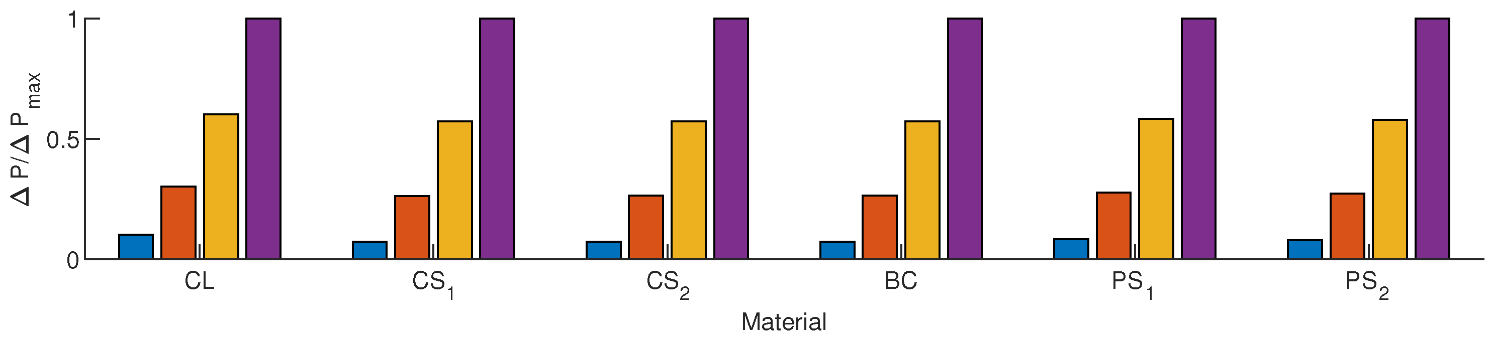Figure 9 shows the $\mathsf{\Delta }P$ for an inlet air velocity of 1.0 m s${}^{-1}$ and a water flow of 6.2 L min${}^{-1}$ m${}^{-1}$. The $C{S}_1$ presents the highest $\mathsf{\Delta }P$ due to the used of the smallest particle size, while the $PS$ pads present the lowest $\mathsf{\Delta }P$, between the alternative pads. The $P{S}_2$ had the lowest value due to the highest particle size. The differences in the $\mathsf{\Delta }P$ values were more noticeable for high u and Q values (data not show).

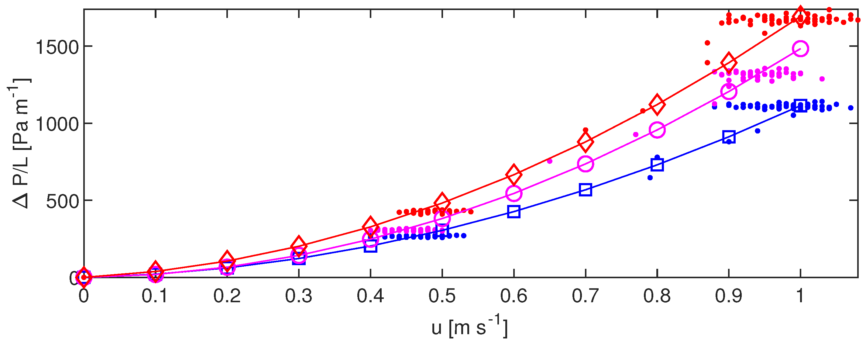
Figure 10 shows the normalized average pressure drop across the different pads tested as a function of the inlet air velocity with a constant water flow of 6.2 L min${}^{-1}$ m${}^{-1}$. As was expected for a porous medium, $\mathsf{\Delta }P$ increased with u. When $\mathsf{\Delta }P$ was normalized with respect to the maximum $\mathsf{\Delta }P$ of each pad material, no visual differences in the behaviour of $\mathsf{\Delta }P$ as u changed were seen. From low to high u, $\mathsf{\Delta }P$ was affected in the same way for all the pads. The relation between $\mathsf{\Delta }P$ and u can be described with the same exponential function, fitted to their respectively $\mathsf{\Delta }P$ values for each pad material.

Figure 11 shows the normalized average pressure drop across the different pads tested as a function of the water flows for a constant inlet air velocity of 1 m s${}^{-1}$. For all the pads, except for the cellulose one, the pressure drop is highly influenced by the water flow through the pad, being the $C{S}_1$ pad the most affected and the $PS$ pad the least affected. The $\mathsf{\Delta }P$ of the cellulose pad changes about 9% due to increasing the water flow, meanwhile the $C{S}_1$ pad changes 80%. In the cellulose material, the water forms a thinner layer in comparison with the alternative pads where it considerably increases the resistance to air flow.

3.6. Permeability

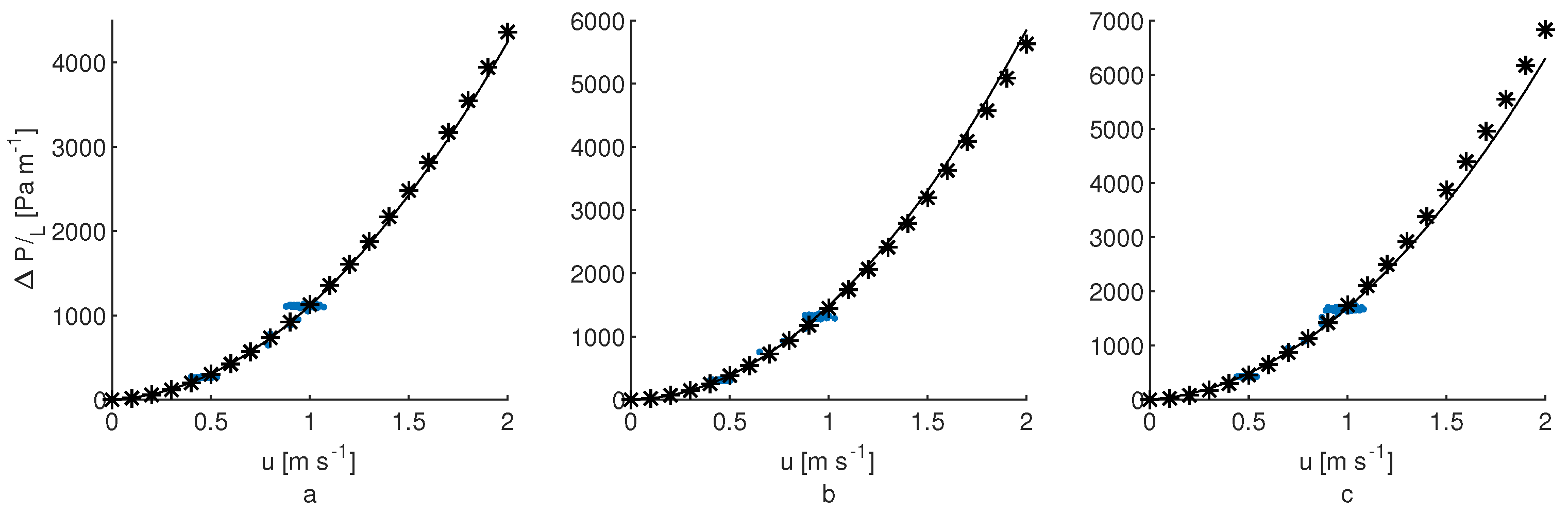
Equation (5) adequately reproduces the relationship between the pressure drop across the pad and inlet air velocity, as is shown in Figure 12 for the $BC$ pad. In this case, the permeability (K) and the Forchheimer coefficient ($\beta$) of the equation were estimated for each water flow used.

To obtain a universal expression to compute the pressure drop across the pad as a function of the inlet air velocity and the water flow, the permeability and the Forchheimer coefficient were considered proportional to water flow, as $K\left(Q\right)=\frac{1}{f_1+f_{2}Q}$ and $\beta \left(Q\right)=(g_1+g_{2}Q)$. Two additional cases were evaluated: assuming that the permeability was water flow dependent or that the Forchheimer coefficient was water flow dependent.

The goodness of the fitted equations was compared through the coefficient of determination (R${}^2$) and the RMSE. The best values were obtained when the permeability was considered constant and the Forchheimer coefficient as a function of the water flow. Figure 13 compares Equation (5) fitted to each water flow when the permeability and the Forchheimer coefficient were considered as constants (solid line), and fitted to all the experimental data (asterisk markers), considering the permeability as a constant and the Forchheimer coefficient as a function of the water flow. There was no visible difference between them for $u<1.0$ and a slight deviation for higher u was detected.

Table 12. Permeability (K) and coefficients used to compute the Forchheimer coefficient as a function of water flow ($\beta \left(Q\right)=(g_1+g_{2}Q)$) in Equation (5). The coefficient of determination ($R^2$) and the Root Mean Square Error (RMSE [Pa]) of the fitted equation are presented. The Forchheimer coefficient for a water flow of 6.2 L min${}^{-1}$ m${}^{-1}$ for comparison purposes is also shown.

Pad	${\mathit{g}}_1$	${\mathit{g}}_2$	${\mathit{R}}^2$	RMSE [Pa]	K [m${}^2$]	$\mathit{\beta }\left(6.2\right)$ [m${}^{-1}$]
$CL$	20.8546	0.2351	0.9997	0.18166	$1.3959\times {10}^{-6}$	22.31
$C{S}_1$	946.7572	72.6893	0.9988	1.36296	$1.0108\times {10}^{-7}$	1397.4
$C{S}_2$	551.5387	39.3833	0.9995	1.05007	$3.6648\times {10}^{-7}$	795.7
$BC$	891.2264	82.1001	0.9991	1.63633	$2.4308\times {10}^{-7}$	1400.2
$P{S}_1$	358.6404	17.9078	0.9995	0.90228	$1.4939\times {10}^{-7}$	469.7
$P{S}_2$	287.9664	9.8696	0.9993	0.85144	$2.6975\times {10}^{-7}$	349.2

summarizes the g’s coefficients, R${}^2$, RMSE, permeability and the Forchheimer coefficient for a water flow of 6.2 L min${}^{-1}$ m${}^{-1}$ for comparison purposes.

As the pad is constantly wetted, the water forms a thick layer over the material, which affects the flow of air, increasing $\mathsf{\Delta }P$. However, the permeability could be considered constant, while the Forchheimer coefficient changes with the water flow. The coefficient $g_2$ shows the effect of the water flow over $\mathsf{\Delta }P$. For the cellulose material, this parameter is small. For the $C{S}_1$ and $BC$ materials this parameter presents significant influence as was shown previously in Figure 11.

The permeability of the alternative materials were ten times lower than that of the cellulose material, which is in the order of $1\times {10}^{-6}$. It was not possible to establish a correlation between the permeability and the magnitude of $\mathsf{\Delta }P$ across the alternative pads. However, this relation is clearly established with the Forchheimer coefficient. This was biggest for $C{S}_1$ and $BC$ pads, which are the ones that produce the highest $\mathsf{\Delta }P$, while the lowest $\beta \left(6.2\right)$ values were obtained for the $PS$ pads, which produces the least $\mathsf{\Delta }P$.

Additionally, there was a big difference between the Forchheimer coefficient of the cellulose and the alternative pads. The Forchheimer coefficient can be considered an indicator of how big the $\mathsf{\Delta }P$ changes are when the inlet air velocity increases. The alternative pads with the biggest particle size ($PS$) present the lowest Forchheimer coefficients, while the $C{S}_1$ pad, which has the smallest particle size, and the $BC$ materials, which have the least porosity, present the maximum values; the effect of the inlet air velocity over $\mathsf{\Delta }P$ is stronger. When the water flow increases, an increase in the resistance to the air flow was also more noticeable on those pads.

4. Discussion

The experimental results showed that the pads evaluated produced cooling efficiencies above 42% and temperature drops up to $5.0{}^{°}\mathrm{C}$, as can be seen in Figure 5 and Figure 7, even with environmental conditions that are not suitable for evaporative cooling (low dry-bulb temperature and high relative humidity of inlet air). The major drawback is the increase in relative humidity that in this case was up to 35%.

The alternative pads presented similar results to those of the cellulose pads. However, the environmental conditions were not kept constant due to experimental limitations, making it difficult to established an unbiased comparison between the pads from the experimental test results. For this reason, the model proposed by Obando et al. [32] was used to simulate each one of the pads in equal environmental and operative conditions. The results presented in Table 8 and Figure 2 show that the model used adequately describes the behaviour of each pad. With this, it was indeed possible to obtain the correlation (3) to compute the convective heat and mass transfer coefficients of each pad, which is useful for performing different thermo-fluid analysis as in Computer Fluid Dynamics simulations. There are few research studies about cooling pads that report those coefficients, ref. [13] being the first one to report the coefficients of the coconut coir fibre and non-woven fabric perforated materials. This study allowed us to confirm that the cellulose pad coefficients were similar to those found by Dhamneya et al. [5], Kulkarni and Rajput [21], Laknizi et al. [30], Franco et al. [56], Chen et al. [57]. The cellulose pad studied in this work serves as reference to validate the model proposed by Obando et al. [32].

Several research studies are in concordance with the inverse correlation of the cooling efficiency and the relative humidity with the air inlet velocity found here [1,24,29]. Although the behaviour of the coconut shield with small particles ($C{S}_1$) was unexpected, some other research studies had documented similar behaviours [12,13,58] with pads based on natural fibres. This behaviour could be attributed to the resistance to the air flow across the pad. For some pads, especially with smaller particle sizes, such as the $C{S}_1$ pad, the particles are arranged in such a way that the high resistance to air flow limits the free transit of the air across the pad, decreasing the surface area in contact with the water. When the inlet air increases, the pressure drop forces the air to flow through small orifices that could be full of water, raising the turbulence of the flow, incrementing the water–air contact and resulting in a drastic decrease in the dry-bulb temperature of outlet air. For the other material that had a lower particle size, the effect is less noticeable.

According to the results shown in Figure 3 and Figure 4, the magnitude of the convective heat and mass transfer coefficients are inversely proportional to the specific surface area found for the alternative pads. That is, those coefficients compensate in some way for the low magnitude of the total wetted surface. On the other hand, alternative pads that had a similar specific surface area to the cellulose one (coconut shells and burnt clay brick) presented the highest cooling efficiency, with a high relative humidity at the outlet, which is also an indicator of high water consumption, while the cellulose pad kept it lower due to its lower convective mass transfer coefficient.

The accuracy of the model results was not affected by not considering the water flow in accordance with [27,28,29,44] or the porosity of the materials as was established by Osorio et al. [16]. It was considered that the water flow was enough to maintain the pads wetted. Water flow beyond the maximum evaporation rate has no beneficial effects [31], and it only affects the pressure drop across the pad, as was shown in Figure 11. So, it is desirable to maintain an equilibrium between the water flow and the evaporative water rate. Similar results were reported by Liao and Chiu [26], Franco et al. [31].

There was a difference above 90% between permeability of the cellulose and the alternative pads, as was reflected in the high pressure drop across these, especially for pads with small particle sizes. Similar pressure drops for alternative materials were reported by Jain and Hindoliya [7], Vijaykumar et al. [14], Basiouny and Abdallah [23], Liao and Chiu [26], Kovács et al. [59].

Based on the Darcy–Forchheimer Equation (5), it was possible to obtain a universal expression for each of the pads analysed to compute the pressure drop in terms of the inlet air velocity and the water flow. Additionally, it was determined that the permeability was not affected by the water flow as it was for the Forchheimer coefficient. Attempts to obtain an expression that describes the relation between inlet air velocity and water flow were made previously by [28,36], adding the characteristic length ($l_e$) without including viscous or inertial force coefficients such as the permeability and the Forchheimer coefficients.

The high pressure drop across the alternative small particle pads made them unfeasible for some applications, even with their high cooling efficiency, because higher exhaust fans are required, increasing the electrical power consumption. Nevertheless, other alternative materials, such as the pumice stones, could be used in applications where a continuous ventilation system with low heat load is required. Those pads could decrease the external temperature by up to $2.0{}^{°}\mathrm{C}$ maintaining a low pressure drop and a low increase in relative humidity.

The pad cooling efficiency is one of the main parameters that had been used to characterize the effectiveness of an evaporative cooling system. However, the use of other quantities made its applicability or benefits to the end user clearer, such as to farmers in agro-industrial facilities. The drop in temperature and the increase in relative humidity in the air leaving the pad provides a clearer idea of the improvement in the thermal conditions of the air. The influence of both variables on the thermal comfort of animals can also be combined in a unique index such as the THI, which gives a better idea of the cooling effect of the thermal comfort of animals inside the facilities, being one of the goals of air conditioning.

The relationship found between the THI, the inlet air velocity and the pad thickness for the cellulose pad were in agreement with the results found previously by Sayed and Khater [39]. Indeed, it was found that, with any of the pads evaluated, it was possible to improve the external thermal conditions of the air maintaining inside the installation a middle thermal comfort zone defined for cattle, up to $T_{d{b}_i}=30{}^{°}\mathrm{C}$ (worst pad behaviour with ${\varphi }_i$ = 60%). If the input relative humidity decreases, it could increase the temperature limit. So, any of the pads could be used to improve the thermal conditions of the air.

When an evaporative system is implemented, it was evident from the results that thicker pads provided higher cooling efficiency. However, this improved with an increasing in the evaporative water rate. When it is going to be used in tropical and subtropical countries such as Colombia, where high relative humidity was predominant, this result is not desirable. So, for these climatic conditions, it is recommended to use pads of 0.1 m of thickness, providing a balance between the dry-bulb temperature drop and the increase in the relative humidity.

5. Conclusions

Using a mathematical model fitted to wind tunnel experimental data, it was possible to perform a complete characterization of several evaporative cooling pads, manufactured with cellulose and alternative materials, in terms of cooling efficiency, Temperature–Humidity Index, dry-bulb temperature drop, relative humidity increment and pressure drop across the pads; as functions of the inlet air velocity, water flow and pad thickness. Pad efficiencies were found between 40% and 70% for pads manufactured with alternative materials for inlet air environmental conditions typical of tropical climate countries like Colombia. The alternative pads with lower particle sizes (higher specific surface area) present cooling efficiencies similar to the cellulose pads (70%) at the expense of a higher pressure drop.

All pads evaluated can improve the inlet air thermal conditions, providing outlet air with Temperature–Humidity Indices below the external environmental conditions and maintaining the mean thermal comfort zone for a broad range of dry-bulb temperatures and relative humidity combinations, making them useful for several applications.

The methodology presented here allows the characterization of new alternative materials in order to find those that provide an adequate balance between cooling efficiency and pressure drop across the pad. Additionally, new simulations can be performed using the convective heat and mass transfer coefficients correlations found for particular conditions.

To decrease the pressure drop across the pads and consequently the electrical power consumption, it is necessary to set the water flow to the minimum value required to maintain the wetted pad, which depends on the evaporation rate, especially when high speeds (above 1.5 m s${}^{-1}$) are used.