SA-GAN: Stain Acclimation Generative Adversarial Network for Histopathology Image Analysis

Abstract

Histopathological image analysis is an examination of tissue under a light microscope for cancerous disease diagnosis. Computer-assisted diagnosis (CAD) systems work well by diagnosing cancer from histopathology images. However, stain variability in histopathology images is inevitable due to the use of different staining processes, operator ability, and scanner specifications. These stain variations present in histopathology images affect the accuracy of the CAD systems. Various stain normalization techniques have been developed to cope with inter-variability issues, allowing standardizing the appearance of images. However, in stain normalization, these methods rely on the single reference image rather than incorporate color distributions of the entire dataset. In this paper, we design a novel machine learning-based model that takes advantage of whole dataset distributions as well as color statistics of a single target image instead of relying only on a single target image. The proposed deep model, called stain acclimation generative adversarial network (SA-GAN), consists of one generator and two discriminators. The generator maps the input images from the source domain to the target domain. Among discriminators, the first discriminator forces the generated images to maintain the color patterns as of target domain. While second discriminator forces the generated images to preserve the structure contents as of source domain. The proposed model is trained using a color attribute metric, extracted from a selected template image. Therefore, the designed model not only learns dataset-specific staining properties but also image-specific textural contents. Evaluated results on four different histopathology datasets show the efficacy of SA-GAN to acclimate stain contents and enhance the quality of normalization by obtaining the highest values of performance metrics. Additionally, the proposed method is also evaluated for multiclass cancer type classification task, showing a 6.9% improvement in accuracy on ICIAR 2018 hidden test data.

1. Introduction

Histopathology image analysis involves the microscopic examination of cancer disease diagnosis using the whole slide imaging (WSI) scanners. In histopathology images, tissue sections are stained with chemical staining agents (i.e., hematoxylin and eosin stains). These agents bind to tissue components and cellular features (e.g., cell and nuclei) [1]. This selective staining of hematoxylin and eosin (H&E) provides invaluable information to pathologists to perform the clinical diagnosis and to characterize various histological specimens. In this process, the pathologists identify specific neoplastic regions based on morphological features and spatial arrangement of cells in pathology images. 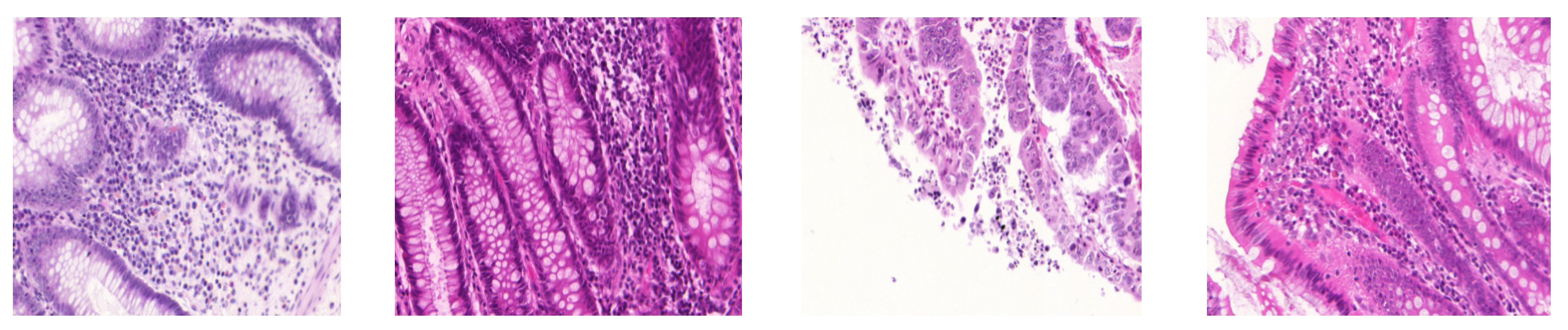Various computer-aided diagnosis (CAD) techniques have been developed to alleviate shortcomings of human interpretations and, therefore, have become valued tools for pathologists [2]. CAD systems provide quantitative characterization of suspicious areas in high resolution H&E-stained histopathology images. The histopathology images often suffer from color and intensity variations, as shown in Figure 1. The main causes of these variations are variability in slide preparation, imprudent staining, operator ability, different slide scanners, and scanning procedures [3]. In the diagnostic field, pathologists can abandon the variability issues but such appearance variations take on great importance in design of automated CAD systems. However, the performance of CAD systems is hampered by such morphological and textural variations [4].

Deep learning [6,7,8] based image analysis algorithms accept that the training (representing source domain) and test (representing target domain) images of any datasets have similar color and texture distributions. It matters, as deep models trained from the dataset with one type of color distribution often fail to work on the dataset with different distributions [9,10]. As said before, color inconsistencies occur in histopathology images. The images originated from different laboratories or even come from a single laboratory show different color distributions. Therefore, deep models trained on training data images are often subtle to color variations of test data. Thus, it is important to condense the intra-laboratory variations between train and test parts of a dataset for training efficient deep models. In this context, so far, several automated stain normalization techniques [11,12,13,14] have been developed to standardize the staining inconsistencies in histopathology images. Such techniques could be used as pre-processing strategies for cancer classification [11,12] and detection [13,14] models to improve the accuracies. However, previously proposed stain normalization algorithms suffer from the errors induced by color channel independence assumption. Moreover, existing methods address the problem of stain normalization by mapping images of a given dataset to a single reference image selected from the target domain. This paper aims to identify whether the color matching algorithms can build an efficient mapping between the two domains by learning the color distribution of whole dataset, instead of relying on a single image.

Based on this objective, we model the stain normalization task as an image-to-image translation task. In the normalization mechanism, color patterns of source domain (training data) are transferred to target domain (test data) while structural contents remain preserved. In this study, we designed a robust generative adversarial network (GAN) based stain transfer strategy, named SA-GAN, which learns the color distributions of entire domain as well as color statistics of a target image instead of just relying only on a single image. The SA-GAN, in a nutshell, contains one generator and two discriminators. The generator model generates images. Among two task-specific discriminators, one enforces the generated image to have the correct color appearance and the second discriminator enforces the texture to be maintained. The SA-GAN network is jointly trained with input training images and a novel metric called color attribute constraint metric extracted from a selected single reference image. Our proposed SA-GAN overcomes the domain adaptation issue by transferring stains across datasets (which describe a similar pathology, having different staining properties). By normalizing the new test data according to training data domain, test images will get color appearance of training images with conserved texture properties. After normalization, feature differences between two datasets become minimized. It is now expected that a classification model trained on training data would be fit for new test data. The designed scheme obtained robust performance in terms of structure preserving and color transferring of histopathology images. The remainder of this paper is organized as follows: Section 2 presents the literature review. A detailed description of the proposed methodology is given in Section 3. Section 4 contains data description, evaluation procedure, results, and discussion. Section 5 concludes the paper.

2. Literature Review

In literature, a large number of state-of-the-art algorithms exist for color standardizing of histopathology images. The color deconvolution methods estimate the staining matrix to decompose RGB images into staining components [15]. The staining matrix represents the concentration of each color stain and can be computed based on image statistics. One of the first non-adaptive color deconvolution algorithm, [15] was proposed to empirically estimate the stain color matrix for hematoxylin and eosin stains. However, this algorithm worsens the normalization performance due to the approximate estimation of stain vectors. Khan et al. [16] introduced a supervised approach to quantify the stain concentration matrix using pixel-level statistical color descriptors (SCD). They used a nonlinear color mapping phenomenon to perform normalization of source image to target image color space. This method involves high computational complexity compared to other state-of-art techniques. Reinhard et al. [17] proposed a color mapping method in LAB color space. In his method, each color channel of source image is aligned to the color channel of user selected template image. After performing the color transformation, the standardized images are converted back to RGB color space. This color matching technique assumes that the proportion of tissue components for each dying agent is similar across the dataset. However, generally, dyes have independent contributions to various tissue images. Consequently, the method by Reinhard et al. [17] leads to improper color matching where the white background is mapped as colored region.

Roy et al. [18] designed a fuzzy based modified Reinhard (FMR) color normalization method to control color coefficients and enhance the contrast of histopathology images. They employed fuzzy logic to overcome the limitation of the conventional Reinhard et al. [17] method. Recently, Vijh et al. [19] proposed a normalization method to reduce the color and stain variability in H&E-stained histopathological images. This method also involves fuzzy logic for illumination, stain, and spectral normalization. Another algorithm by Macenko et al. [20] finds the singular value decomposition (SVD) values in the optical density space and projects the data onto the plane that corresponds to the two largest singular values. This technique can be applied to other histological stains and implicates low computational complexity. However, it becomes possible to wrongly estimate the stain vectors when the intensity of the stained region becomes higher than the imposed threshold (β = 0.15). Shafiei et al. [21] proposed a normalization approach based on the previously introduced spatially constrained mixture model [22]. In [22], a multivariate skew-normal distribution was used to quantify symmetric and nonsymmetric distributions of the stain components and to estimate the parameters. Recently, Salvi et al. [23] proposed an unsupervised normalization technique named the stain color adaptive normalization (SCAN) algorithm. The SCAN algorithm is based on segmentation and clustering strategies. In addition, Pérez-Bueno et al. [24] proposed a method for blind color deconvolution of histology images based on the total variation (TV) technique. They used variational Bayesian algorithm to compute stain concentration and color matrix. The presence of strong color variations in H&E-stained histology images cause the failure of this algorithm. Recently, Hoque et al. [25] designed a color deconvolution technique to quantify the stain components from H&E-stained images. The Retinex model [25] determines an illumination map that is constructed using the maximum intensity of RGB color channels. Zheng et al. [26] proposed an algorithm named adaptive color deconvolution (ACD) for stain separation and color normalization of whole slide images (WSIs). The ACD model [26] is an optimization strategy to estimate the stain separation parameters by considering different prior knowledge of staining (i.e., proportion of stains and intensity). The advantage of this approach is to reduce the failure rate of normalization, but it involves high optimization costs.

As per the literature, two main types of color normalization methods exist: standard color deconvolution methods and generative adversarial network (GAN) based color transfer methods. In standard color deconvolution methods, a single image is selected as a reference image and color distributions of all source images are mapped to that single image. It is accepted that if someone selects a single image the color characteristics of that image are copied to all source images. This type of color transformation creates color artifacts in the processed images.

Recently, GAN-based methods effectively solve the problems of image super-resolution, reconstruction, and segmentation, and are widely used for many medical image analysis tasks. Additionally, different generative adversarial networks (GANs)- [27] based stain transfer techniques [28,29,30,31] have been proposed for color normalization of histopathology images. Although the simple GAN network shows significant performance on natural images; it is however, not proficient to maintain the structural contents in histopathology images. The aforementioned GAN-based methods involve a group of images in color transfer process. So, they efficiently learn dataset-specific properties but ignore image-specific color patterns in the histopathology images. In this paper, we propose a novel design that modeled the stain normalization as an adversarial game and transfer stains across datasets, originating from different pathology laboratories with different staining appearances. Specifically, we aim to design a fully trainable framework that not only transfers stains across the datasets but also learns to easily adjust color attributes of processed images. The trained model would ultimately condense the stain variations in image datasets by leveraging dataset distributions as well as color attributes details extracted from the reference image. It is important to clarify that color attribute metrics are employed to control the color and contrast characteristics of the generated images. Using the color attribute details, our proposed method easily adjusts color contents and preserves structural details in the processed images. Simultaneously, it reduces the inter-variability of background color among the processed images. We argue that incorporating the color attributes and generative adversarial learning into a unified framework achieves high quality color normalization results. To the best of our knowledge, this is the first stain transfer method that incorporates the color attribute details with deep GAN network. Proposed SA-GAN is publicly available at: https://github.com/tasleem-hello/SA-GAN/tree/main.

The main contributions of this work are summarized as follows:

• In this paper, color accumulation task is formulated as an unpaired image-to-image translation task. We aim to modify the color patterns of training data similar to the test images, without changing their structural details.
• We propose a novel stain acclimation network named SA-GAN, with one generator and two discriminators which are trained with two adversarial losses and one textural loss in adversarial and transfer training steps, respectively.
• The designed SA-GAN network is jointly trained with input training images and a novel metric called color attribute constraint. Incorporating the color attribute constraint and generative adversarial learning into a unified framework, correctly transfers the color contents and creates visually realistic images.
• The trained model works effectively for histopathology datasets of different statistical properties (i.e., different staining appearances originating from different pathology centers). Experimental results showed that our proposed SA-GAN outperforms the state-of-the-art by transferring the stain colors across the datasets efficiently.

3. Methodology

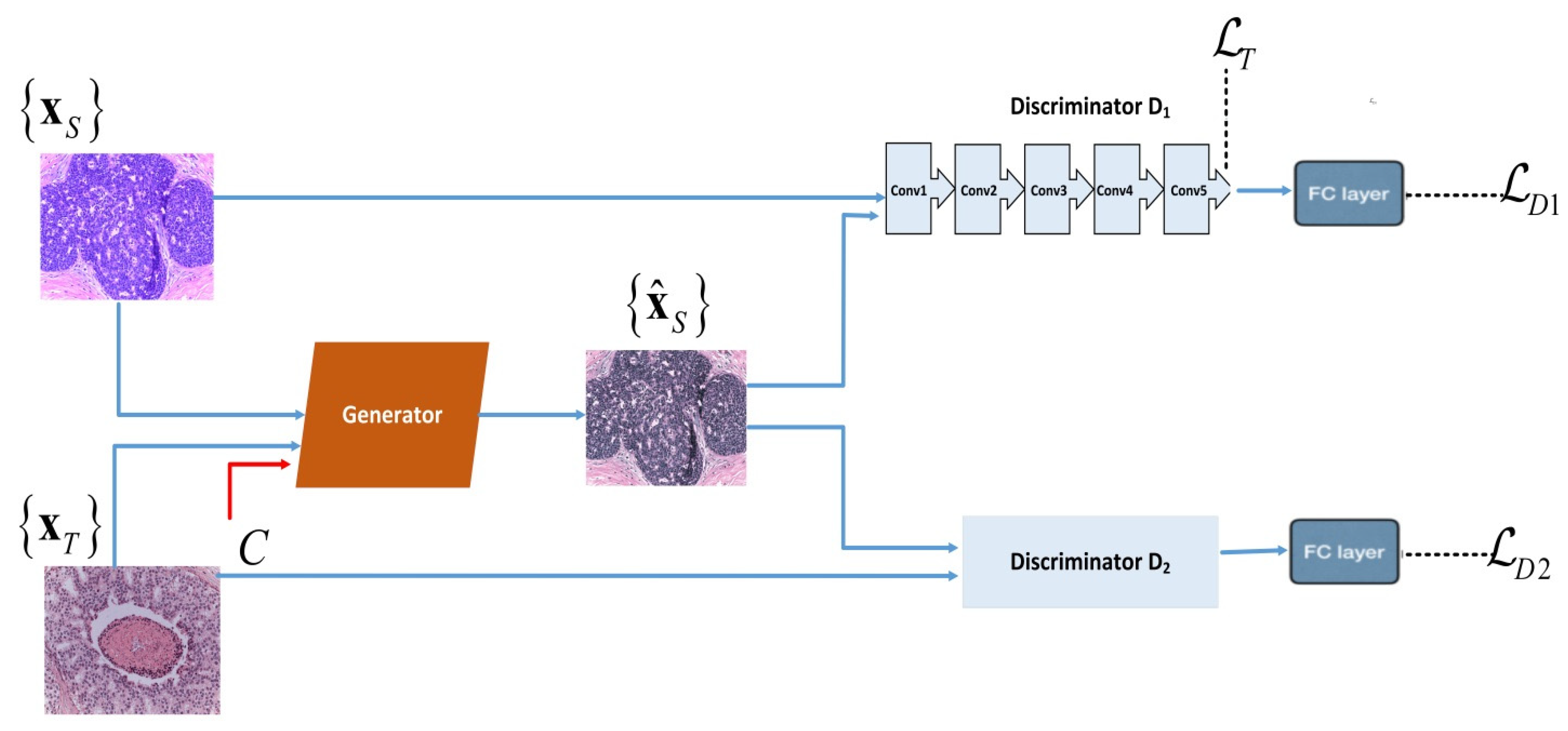
Model Formulation: We designed the architecture of our SA-GAN color transfer network by using convolution neural networks. In proposed SA-GAN, the style transfer task is performed with generator network G that competes against two discriminators, D₁ and D₂. The generator contains an encoder of two convolution blocks (each block includes 2D convolutional layers, instance normalization layers and Leaky ReLu activation functions, sequentially) and a decoder of two transpond convolution blocks (each block includes transposed convolutional layers, instance normalization layers and ReLu activation functions). The generator also contains nine residual blocks similar to that in [30], which improve the quality of the image translation task [31]. Each residual block is composed of two 2D reflection padding layers, two 2D convolution layers, two instance normalization layers, a ReLu activation function, and a plus operation, sequentially. Among discriminators, the first discriminator D₁ maintains the color patterns of the target domain in generated images. While second discriminator D₂ preserves the structure details of the source domain in generated images. These two discriminators (D₁ & D₂) have similar architectures of four convolutional blocks (including a 2D convolution layer, instance normalization layer, and the ReLu activation function) and are followed by a fully connected layer. The workflow diagram of SA-GAN is shown in Figure 2.

Color attribute constraint metric: Two types of stains are used in histopathology images, i.e., hematoxylin and eosin (H&E) stain. Hematoxylin stains the nuclei and eosin mainly stains the cytoplasm and stroma tissues. The majority of pixels in images alternatively contain H or E stains and a third channel called residual channel D, which should be zero in the ideal situation. Thus, it is considered that proportion of the two stains and overall intensity of staining is equally important for the normalization. In our proposed design, to correctly condense the stain variations in the dataset and to easily adjust color attributes (contrast and brightness) of processed images, we selected an image $I\to {ℝ}^{M\times N\times 3}$ from target domain and computed its color attribute metric C. A color attribute metric for each stain $C\to {ℝ}^{k\times 3}$ is calculated by applying color deconvolution (CD) method using Beer–Lambert law [32]. CD can be briefly represented with the following equations:

$$D=-\frac{\ln (I)}{I_{\max }}$$

(1)

$$C=AD$$

(2)

where $I_{\max }$ denotes maximum of digital image intensity (i.e., 255 for 8-bit data format). The $D\to {ℝ}^{k\times 3}$ denotes the optical density (OD) of RGB channels, $A\to {ℝ}^{3\times 3}$ is a so-called color deconvolution matrix that can be manually measured using an experiment reported in [32]. $C\to {ℝ}^{k\times 3}$, in Equation (2), represents the output that contains stain densities. For H&E-stained image, separate densities of stains can be represented as $C={(H,E,D)}^T$ where H&E are the values for hematoxylin and eosin stains, respectively, and D represents the residual of the separation. We named the stain densities matrix $C\to {ℝ}^{k\times 3}$ as color attribute constraints metric. We encoded numerical values of color constraint metric $C\to {ℝ}^{k\times 3}$ as a feature plane with the selected target image. In training, the encoded values are input to the encoder of the deep SA-GAN model as additional information to correctly adjust the color details of generated images.

Problem Setting: We define a set of unseen test data as $\left\{x_S\right\}$ comes from a source pathology center and a set of labeled training data as $\left\{x_T\right\}$ with annotations (either for mitosis cell detection task or for cancer type classification task) comes from a target pathology center. It is assumed that source images $\left\{x_S\right\}\in A$ belong to domain A and target images $\left\{x_T\right\}\in B$ belong to domain B. The images of both domains have different color appearances due to the originating from different pathology centers. Our objective is to transfer $\left\{x_S\right\}$ from domain A to domain B: ${\widehat{x}}_S$ such that generated images $\left\{{\widehat{x}}_S\right\}$ have textural content as in A and color pattern as in B.

Training Functions: Given a histopathology image $x_S$ and color attribute metric C the generator G generates new image ${\widehat{x}}_S=G(x_S,C)$. Among the two discriminators, first discriminator D₁ is optimized to distinguish texture details between the generated images $\left\{{\widehat{x}}_S\right\}$ and source images $\left\{x_S\right\}$ by minimizing texture content loss ${ℒ}_{D1}$, and second discriminator D₂ is optimized to distinguish the color contents between generated images $\left\{{\widehat{x}}_S\right\}$ and target images $\left\{x_T\right\}$ by minimizing the color content loss ${ℒ}_{D2}$. Further, for satisfactory preservation of texture details in generated images, we propose to compute third loss, i.e., textural loss ${ℒ}_T$. ${ℒ}_T$ loss is calculated from feature maps of the last convolution layer of the discriminator D₁. Two adversarial losses (${ℒ}_{D1}$,${ℒ}_{D2}$) and one textural loss (${ℒ}_T$) are combined to train the generator G. Aforementioned GAN performs properly on natural images [27]. However, the main objective of stain transfer in histopathology images is not just to extract the information but also to maintain the content details (color and texture). Hence, we believe that ${ℒ}_{D2}$, ${ℒ}_{D1}$, and ${ℒ}_T$ losses are more realistic metrics for efficient stain transfer in histopathology images.

Conventional methods achieved color normalization by matching the color statistics of source images $\left\{x_S\right\}$ to a single reference image $x_T$. The proposed network learns to generate images by involving staining properties of the entire domain of images $\left\{x_T\right\}$ instead of relying only on single image $x_T$. This implies learning the probability distribution of images $\left\{x_T\right\}$, which can be achieved by computing the two adversarial loss functions, i.e., ${ℒ}_{D1}$ and ${ℒ}_{D2}$.The adversarial losses involve the generator G(x) that maps an input source image $x_S$ to generate stain normalized image ${\widehat{x}}_S$. The losses also involve two discriminators D₁(G(x)), and D₂(G(x)) which simultaneously outputs the likelihood of given input images $x_S$ and $x_T$ to be sampled from source and target sets, respectively. These losses are used to train the generator (including the encoder and decoder) and discriminators. Formally, adversarial losses are described as:

$${ℒ}_{D1}(G, D_1)={\mathbb{E}}_{x\sim \left\{x_S^n\right\}}[log{D}_1(x)]{\begin{array}{l}+{\mathbb{E}}_{x\sim \left\{x_S^n\right\}}[log(1-D_1(G(x)))]\hfill \end{array}}_{}$$

(3)

$${ℒ}_{D2}(G, D_2)={\mathbb{E}}_{x\sim \left\{x_T^n\right\}}[log{D}_2(x)]\begin{array}{l}+{\mathbb{E}}_{x\sim \left\{x_S^n\right\}}[log(1-D_2(G(x)))]\hfill \end{array}$$

(4)

Adversarial learning aims to preserve structural details. To this end, it is assumed that generator learns to reconstruct the input images. Since optimization goals of two adversarial losses are contradictory. Therefore, the textural loss ${ℒ}_T$ is computed from the last convolutional layer of the discriminator D₁, which helps to satisfactorily preserve the structural details. ${ℒ}_T$ loss is defined as follows:

$${ℒ}_T(G)={\mathbb{E}}_{x\sim \left\{x_A^n\right\}}\Vert ℱ{(G(x))}^{(D_1,l)}-ℱ{(x)}^{(D_1,l)}{\Vert }_F$$

(5)

where $\Vert {\Vert }_F$ represents the Frobenius norm. To compute the texture loss ${ℒ}_T$, we use the discriminator D₁ instead of D₂. The reason behind this is that in adversarial training the discriminator D₂ pays too much attention to the color transformation and does not focus on textural details. Therefore, D₂ is not considered appropriate to compute ${ℒ}_T$ loss. The SA-GAN is designed by combining the color attribute constraint C, textural loss, and two adversarial losses to transform the desired color values between the images of different domains while preserving the structural details. The full objective of the SA-GAN is formulated as:

$$ℒ(G, D_1,D_2)=\alpha {ℒ}_T(G)+\beta {ℒ}_{D1}(G, D_1)+\gamma {ℒ}_{D2}(G, D_2)$$

(6)

where α is weight factor to control textural loss, β and γ are the hyperparameters for balancing of two adversarial losses.

We aim to solve:

$$G^{\ast }=arg \underset{G}{min}\underset{D_1,D_2}{max}ℒ(G, D_1, D_2)$$

(7)

Training of the SA-GAN model commensurate with color attribute constraints modifies colors of generated images. The training steps of the optimization procedure are given in Algorithm 1.

Algorithm 1 SA-GAN Optimization Algorithm

4. Experimental Results

In this section, the proposed SA-GAN and other stain normalization methods designed from different aspects are compared and discussed. The compared state-of-the-art methods are implemented in python, running on an Intel^® Xeon^® CPU E5-1620 v3 PC with 3.54 GHz CPU with one NVIDIA Tesla M40 GPU of 12 GB memory. However, for the implementation of the proposed SA-GAN model, the PyTorch library was used. To optimize the generator and discriminators of the SA-GAN model, we applied the Adam optimizer using the batch size of 1. We α = 0.001, β = 0.01, and γ = 0.01, so that two discriminators can perform a major role in the training of feature extractors, while minorly taking part in training of generator. The whole model was trained using a learning rate = 0.0002. For experimental analysis, three publicly available breast cancer [33,34,35] and one colon cancer [5] datasets were used. The detailed description of datasets is given as follows:

The mitos & amp; atypia 14 (MITOS-ATYPIA-14) challenge dataset [33]: This dataset includes 1200 training and 496 test HPF images. Annotations of training data are available but annotations of test data are withheld by organizers. The HPF images were scanned with two AperioXT and Hammatsu Nanozoomer 2.0-HT scanners at ×40 magnifications. We checked the model performance on HPFs that are scanned by AperioXT scanner. The size of these images is 1539 × 1376 pixels. The training and test sets have larger appearance variability in images in terms of texture contents and staining properties.

The tumor proliferation assessment challenge (TUPAC 2016) challenge dataset [35]: The auxiliary dataset contains images of 73 breast cancer patients arising from three different pathology centers. Among 73 training cases, the first 23 correspond to the previously released AMIDA13 contest dataset [36]. These cases are obtained from the pathology center at the university medical department in Utrecht. The remaining 50 cases come from the other two different pathology labs in the Netherlands. These images were produced with the Leica SCN400 scanner at ×40 magnification with spatial resolution of 0.25 µm/pixel. The annotations were labeled by two different pathologists. The annotations of training data are publicly available while annotations of test data are not yet available.

The ICIAR 2018 breast cancer histology (BACH) grand challenge dataset [34]: This dataset is provided as a part of international conference on image analysis and recognition (ICIAR 2018) breast cancer histology challenge. It contains 400 training and 100 test H&E-stained microscopy images of 2048 × 1536 × 3-pixel resolution. Images are scanned by LeicaDM 2000 LED microscope of 0.42 × 0.42 μm/pixel resolution. These images were labeled by two expert pathologists into four classes. Labels of training images are available; however, labels of test images are withheld by the organizers. Large color variability exists in this data, so this dataset is more appropriate for the color normalization task and to evaluate the performance of automatic cancer diagnostic systems. We used this dataset to perform the multiclass classification of breast histopathology images: normal, benign, in situ, and invasive carcinoma classes.

MICCAI’16 gland segmentation (GlaS) challenge dataset [5]: This dataset is provided as a part of international conference on medical image computing and computer assisted intervention (MICCAI 2016) gland segmentation challenge. The training dataset contains 85 H&E colon adenocarcinoma tissue images, 37 belong to benign tumors, and the remaining 48 belong to malignant tumors category. The test data consist of 80 test images; 37 belong to benign tumors and 43 to malignant tumors. The spatial resolution of these images is 775 × 522 pixels, which were scanned by Zeiss MIRAX MIDI scanner of 20× (0.62005 µm/pixels) magnification.

In this paper, the performance of our proposed algorithm is compared with five state-of-the-art approaches proposed by Khan et al. [16], Macenko et al. [20], Reinhard et al. [17], Zheng et al. [26], and Shaban et al. [28]. Several popular performance metrics in the field are used to analyze the efficiency of different color normalization methods. These metrics help to decide a method that could be most suitable for color normalization of histology images. To analyze the texture contents of processed images, the similarity metrics such as structural similarity index (SSIM) [37] and Pearson correlation-coefficient (PCC) [37] are computed. Moreover, performance of the proposed method is checked in terms of coefficient of variation of normalized median intensity (CV-NMI) [38] and normalized median hue (CV-NMH) [39]. Meanwhile, inter and intra color variations in training and test dataset were analyzed by evaluating the histogram correlation [40] and Bhattacharyya distance [41] metrics. The computed metrics measure the color and structural variability within a dataset and also help to infer the datasets, which could be more feasible to train an efficient deep CNN model. Detailed description of these quality metrics is given in the following subsections.

4.1. Structure Analysis

Evaluation metrics: The Pearson correlation-coefficient (PCC) [37] [1], structural similarity index (SSIM) [37] and peak signal-to-noise ratio (PSNR) [42] are taken to evaluate structural analysis. Texture properties of histology images are related to spatial distribution of image intensity values. We quantified the texture similarity between the original and processed images by computing PCC metric. A PCC of value 1 implies that intensity distributions of original image are exactly preserved in the processed image, which is highly desirable in color normalization. On the contrary, PCC of value 0 denotes that no similarity occurs between the images. PCC is described as:

$$PCC=\frac{{\displaystyle \sum _i(a_i-{\mu }_a)(b_i-{\mu }_b)}}{\sqrt{{\displaystyle \sum _i{(a_i-{\mu }_a)}^2\sqrt{{\displaystyle \sum _i{(b_i-{\mu }_b)}^2}}}}}$$

(8)

where a_i and b_i represent source and processed images, respectively. μ_a and μ_b represent the mean of source and processed images, respectively. Similarly, the SSIM [37] metric is calculated to measure structural, contrast, and luminance differences between two images. For robust normalization, SSIM value should be close to one. SSIM is described as:

$$SSIM(a,b)=(\frac{2{\mu }_a{\mu }_b+x_1}{{\mu }_a^2+{\mu }_b^2+x_1})(\frac{2{\sigma }_{ab}+x_2}{{\sigma }_a^2+{\sigma }_b^2+x_2})$$

(9)

where σ_a and σ_b are the standard deviation of source and processed images, respectively. σ_ab is the correlation between source and processed images. x₁ and x₂ are the constants used to stabilize SSIM when its value approaches zero. Furthermore, to analyze the perceptual quality of stain transferred image, $PSNR=20\log MA{X}_I/\sqrt{MSE}$ score is computed, where MAX_I is the maximum intensity value in the image and MSE is the mean squared error between stain transferred image and target (test) image.

Qualitative and quantitative performance: In this analysis, we discussed the qualitative and quantitative normalized performance of proposed method. The qualitative results of the proposed SA-GAN and other state-of-the-art methods are given in Figure 3. Visual inspection depicts that when the images are processed with stain color descriptor (SCD) [16] method, white luminance part is not well preserved but structural details are maintained to some extent. Results obtained with Macenko [20] method show that color from target image is not transferred correctly and the white background of source image is fraught with fade color. Nevertheless, the Macenko method effectually avoided structural artifacts. Reinhard et al. [17] method maintained the structural details of the source image; however, color contents are not transferred properly from source to processed image. The SCD [16] method does not maintain the structure and color details in processed images. Compared to all other benchmark methods, in SCD method, loss of information is high, and more structural defects occur for all datasets that can be particularly seen in Figure 3. In contrast, results obtained with the adoptive color normalization (ACD) [26] method preserve the structure details. However, the color information is not exactly transferred to processed images, and the background of images is also affected.

Staining of the bright background luminance, tint, or discoloration of nuclei appears in many normalized images across all the datasets. For instance, the SCD and Macenko method stains bright backgrounds, and color characteristics of target domain are copied to normalized colon cancer images and also are seen in the breast cancer ICIAR dataset images. Artifacts such as stained bright background or improper color in nuclei appear in the results of the StainGan [28] method. The processed images with accurate stain representations and structural details are considered the best results. Hematoxylin appears as the predominant color in the nuclei, while eosin appears in the stroma or other organs. From visual analysis, it is clear that our method overcomes all the limitations of prior proposed conventional methods. It is mainly due to the involvement of color distributions of entire image domain as well as the use of the color attribute metric.

The quantitative color normalization performance of tested methods on various datasets is given in

Table 1. Comparison of PSNR of different color normalization methods using various histopathology datasets.

Datasets	SCD [16]	Macenko [20]	ACD [26]	Reinhard [17]	StainGan [28]	SCAN [23]	Proposed Method
MITOS-ATYPIA-14	26.01	25.03	23.01	29.03	30.01	29.7	33.02
TUPAC 2016	26.04	28.04	24.02	30.04	31.04	30.2	34.08
ICIAR 2018	29.07	27.07	25.05	31.05	29.09	32.6	33.07
MICCAI’16	28.02	28.06	22.04	31.08	31.02	31.1	35.03

and

Table 2. Comparison of PCC and SSIM for different color normalization methods.

Datasets	SCD [16]		Macenko [20]		ACD [26]		Reinhard [17]		StainGan [28]		SCAN [23]		Proposed Method
	PCC	SSIM	PCC	SSIM	PCC	SSIM	PCC	SSIM	PCC	SSIM	PCC	SSIM	PCC	SSIM
MITOS-ATYPIA-14	0.868	0.750	0.830	0.854	0.902	0.891	0.932	0.957	0.882	0.891	0.861	0.912	0.960	0.940
TUPAC 2016	0.868	0.750	0.885	0.931	0.921	0.892	0.970	0.931	0.941	0.952	0.894	0.887	0.951	0.910
ICIAR 2018	0.851	0.742	0.871	0.902	0.953	0.862	0.954	0.961	0.970	0.915	0.910	0.892	0.981	0.992
MICCAI’16	0.932	0.925	0.892	0.897	0.912	0.910	0.891	0.942	0.932	0.921	0.889	0.910	0.982	0.972

. In comparison to the previous methods, our method shows remarkable PSNR on all datasets. The evaluated parameters (PCC and SSIM) with prior proposed methods, widely deviate from one for all breast and colon datasets. Lower and positive values of PCC and SSIM are non-ideal. Small PCC values demonstrate that color inconsistencies are still present in processed images. Similarly, the low value of SSIM obtained with other methods indicates that structure details are not well preserved in stain normalized images. The large difference between values of SSIM and PCC represents that the normalization methods are inconsistent in producing images with accurate contrast. Some of the processed images have enhanced contrast while other images have low contrast value. Compared to state-of-the-art algorithms, our method not only obtained high PCC and PSNR values but also achieved a remarkable value of SSIM.

The quantitative (Table 1 and Table 2) results reveal that the designed algorithm outperforms all prior and recently proposed state-of-the-art color normalization algorithms [16,17,20,23,26]. For our method, the measured SSIM and PCC values (Table 2) are very close to one for all datasets. In visual analysis in Figure 3, images that show accurate stain representations are considered the best stain normalized results. The visual assessment shows that significant improvements in color consistency occur and no apparent artifacts are found in the results of the SA-GAN model. From qualitative results, it is also apparent that our designed stain transfer algorithm is robust and applicable to H&E-stained histology images.

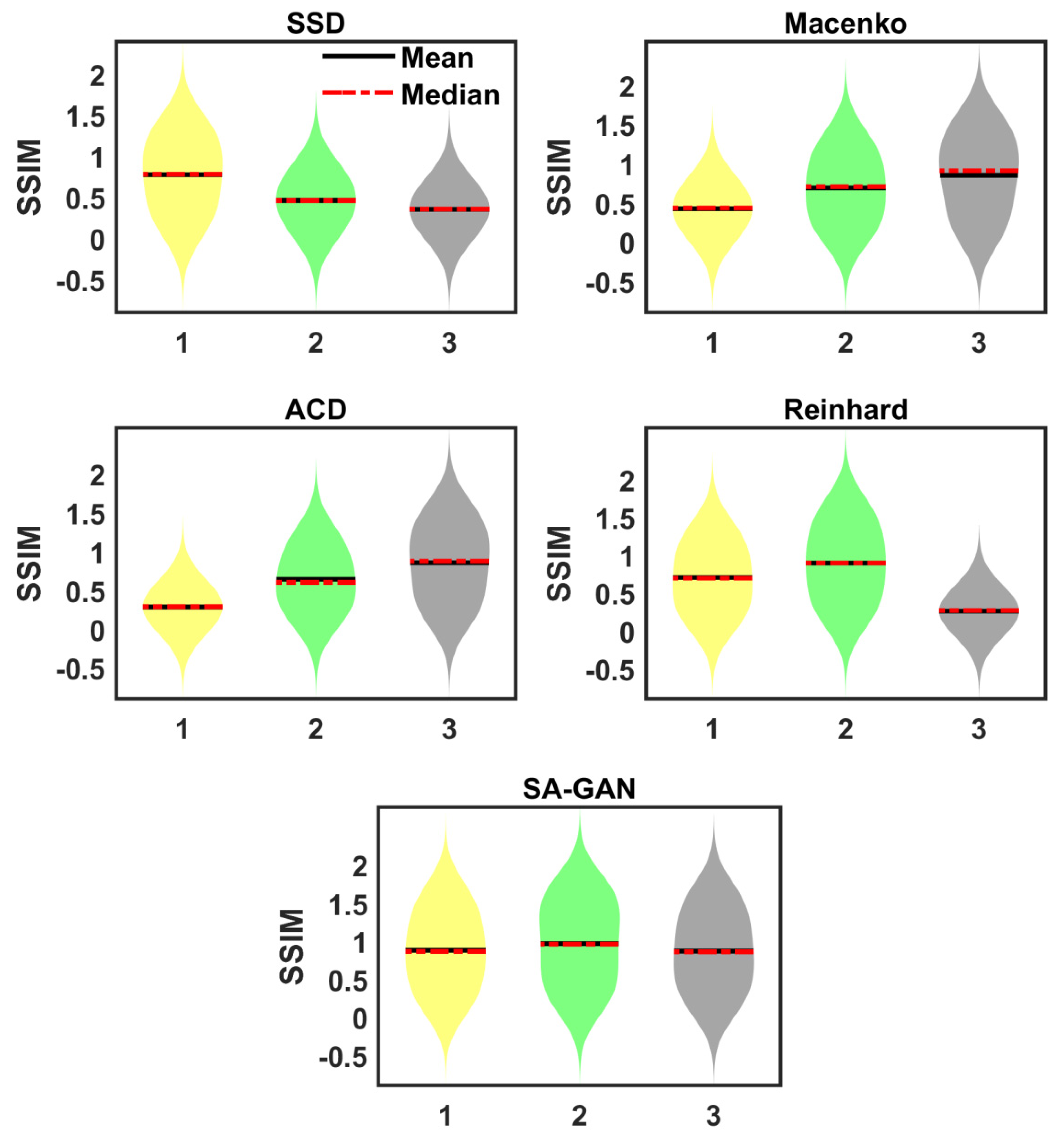
Sensitivity towards different target images: In this analysis, the sensitivity of color mapping methods to choose the target image is checked. We selected three different target images from ICIAR 2018 dataset [34]. Correspondingly, three different color attribute metrics are computed from selected images. The SA-GAN model is separately trained using computed color metrics. We did not observe any change in SSIM value by changing the color metrics. However, color attribute constraint information assists in adjusting the colors of generated images properly. It is noticed that previously proposed color mapping methods [16,17,20,26] are sensitive towards the selection of target images. Results evaluated with other methods represent the change in SSIM regarding target images (Figure 4). This is because these methods use a single image in color normalization process, whereas our designed strategy takes advantage of whole dataset distributions as well as color statistics of a single target image instead of just relying on a single image.

4.2. Inter Datasets Color Constancy Analysis

In this section, influence of proposed SA-GAN algorithm on the stain color differences between different datasets originated from different laboratories has been observed. Stain color variations across the datasets are checked in terms of color consistency using normalized median intensity (NMI) [38] metric. NMI is used to measure stain color intensities of nuclear and eosin regions. NMI is defined as:

$$NMI(I)=\frac{median\left\{I(i)\right\}}{P_{95}\left\{I(i)\right\}}$$

(10)

where I(i) is the mean of R, G & B channels of image I for pixel i and denominator denotes 95th percentile However, NMI specifies the image’s intensity information more than the color contents. So, to measure variability in hue color across the datasets, we quantified a specific color consistency metric, i.e., normalized median hue (NMH). NMH is a novel color metric recently proposed in [39]. NMH is defined as:

$$NMH(h)=\frac{median\left\{H(h)\right\}}{P_{95}\left\{H(h)\right\}}$$

(11)

where the numerator is median of hue channel of HSV image and denominator is 95th percentile of hue channel for pixel h.

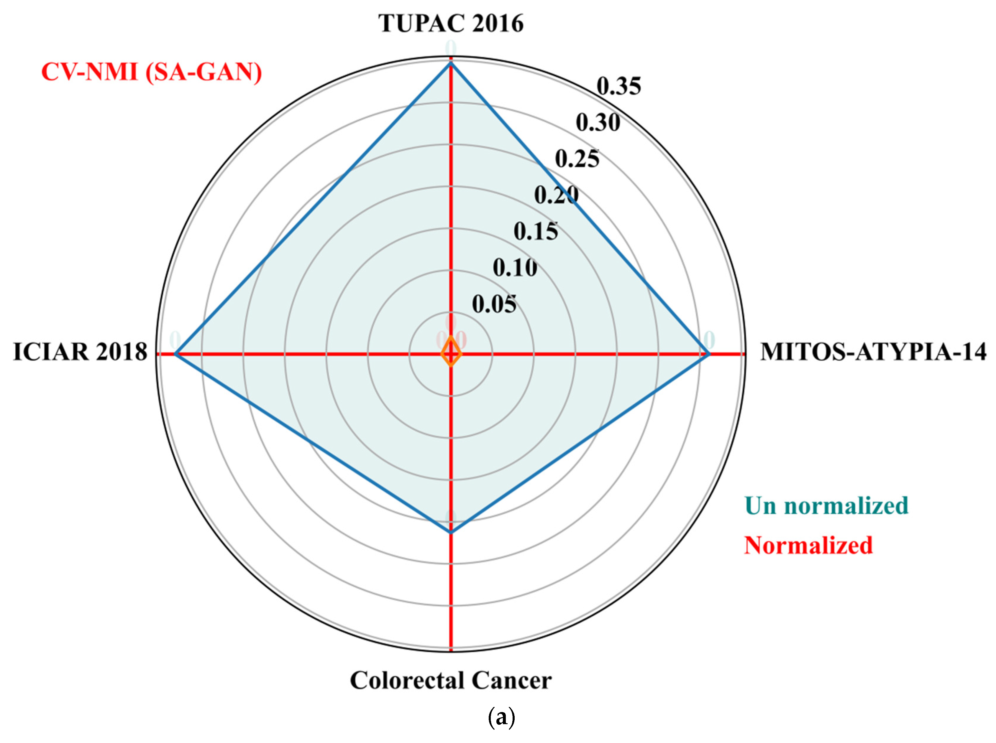
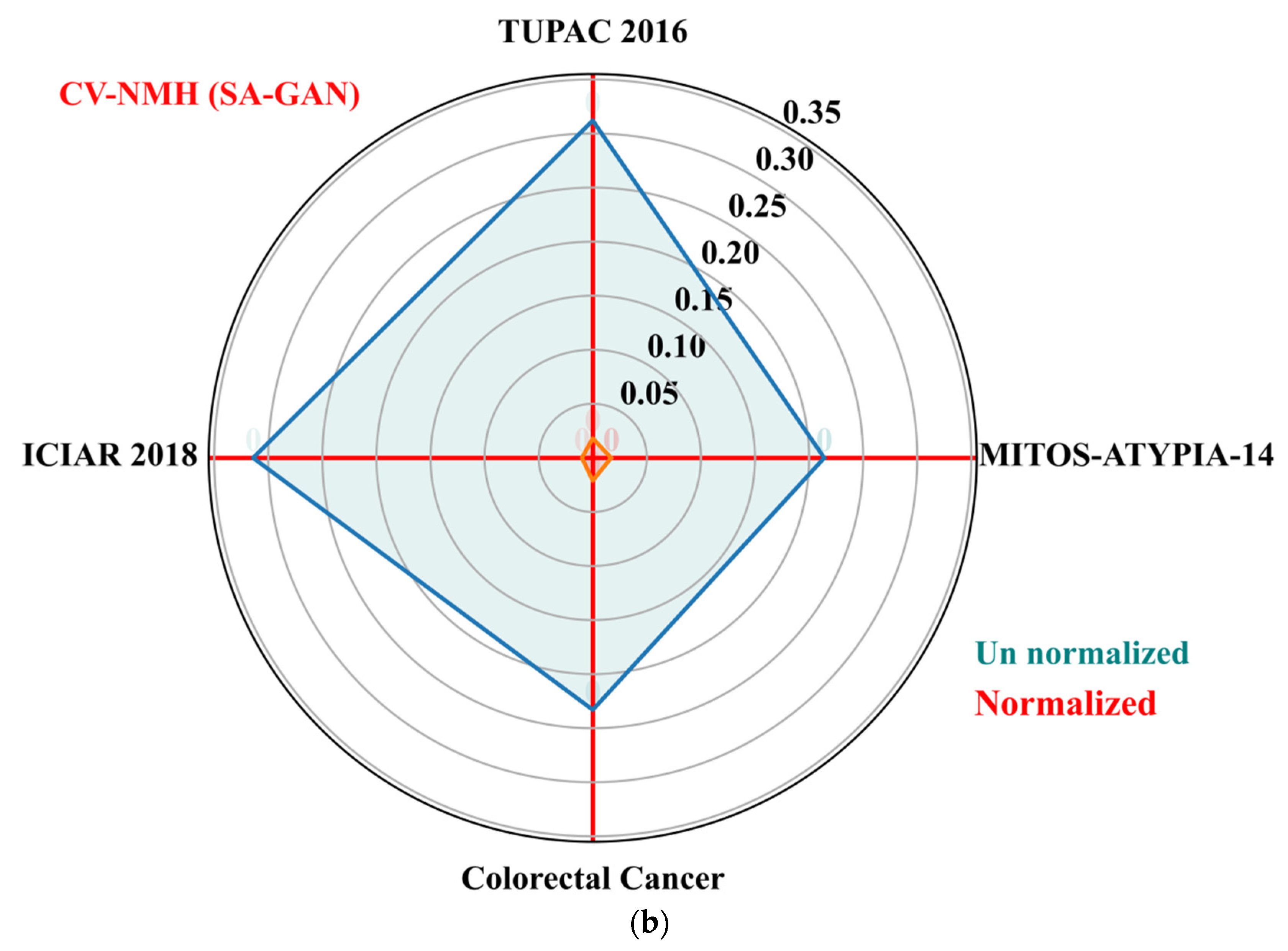
The goal of these metrics is to determine the variation of color distributions across a population of images. We also computed population variability metric, i.e., coefficient of variation (CV) across train and test sets of each dataset. The CV (standard deviation divided by mean) is computed separately for NMI and NMH metrics from each dataset. The low value of CV-NMI and CV-NMH indicates that fewer image intensity variations and low color variability exist within an image population. The CV of NMI and NMH for the proposed SA-GAN algorithm are computed and compared amongst the normalized image sets to un normalized sets and plotted the results in Figure 5a,b. The polar plane results show the optimal values of CV-NMI and CV-NMH for normalized datasets in comparison to un normalized datasets. These optimal values indicate that after the stain transfer, the processed images have less population variability. In polar plots, the clustering effect of our SA-GAN algorithm for normalized datasets can also be confirmed. Moreover, comparison of measured metrics values for various normalization algorithms [16,17,20,23,26] on all tested datasets are given in

Table 3. Evaluation of stain accumulation in terms of CV-NMI and CV-NMH.

Normalization Method	MITOS-ATYPIA-14		TUPAC 2016		ICIAR 2018		MICCAI’16
	CV-NMI	CV-NMH	CV-NMI	CV-NMH	CV-NMI	CV-NMH	CV-NMI	CV-NMH
No normalization	0.311	0.214	0.347	0.312	0.332	0.314	0.213	0.233
SCD [16]	0.142	0.132	0.123	0.102	0.131	0.120	0.103	0.124
Macenko [20]	0.089	0.092	0.0901	0.083	0.082	0.078	0.087	0.082
ACD [26]	0.071	0.089	0.073	0.871	0.078	0.0871	0.076	0.076
Reinhard [17]	0.042	0.030	0.042	0.021	0.043	0.034	0.033	0.032
StainGan [28]	0.031	0.029	0.035	0.032	0.298	0.032	0.027	0.028
SCAN [23]	0.041	0.032	0.039	0.047	0.040	0.035	0.039	0.038
Proposed SA-GAN	0.012	0.017	0.021	0.018	0.011	0.010	0.014	0.021

. Low values of CVs (Table 3) represent the proxy measurement of quality of proposed SA-GAN method, compared to other normalization methods. Minimization of coefficient of variation of NMI and NMH in normalized image datasets is the indication of color consistency across the datasets which improves the classification performance of deep CNN models.

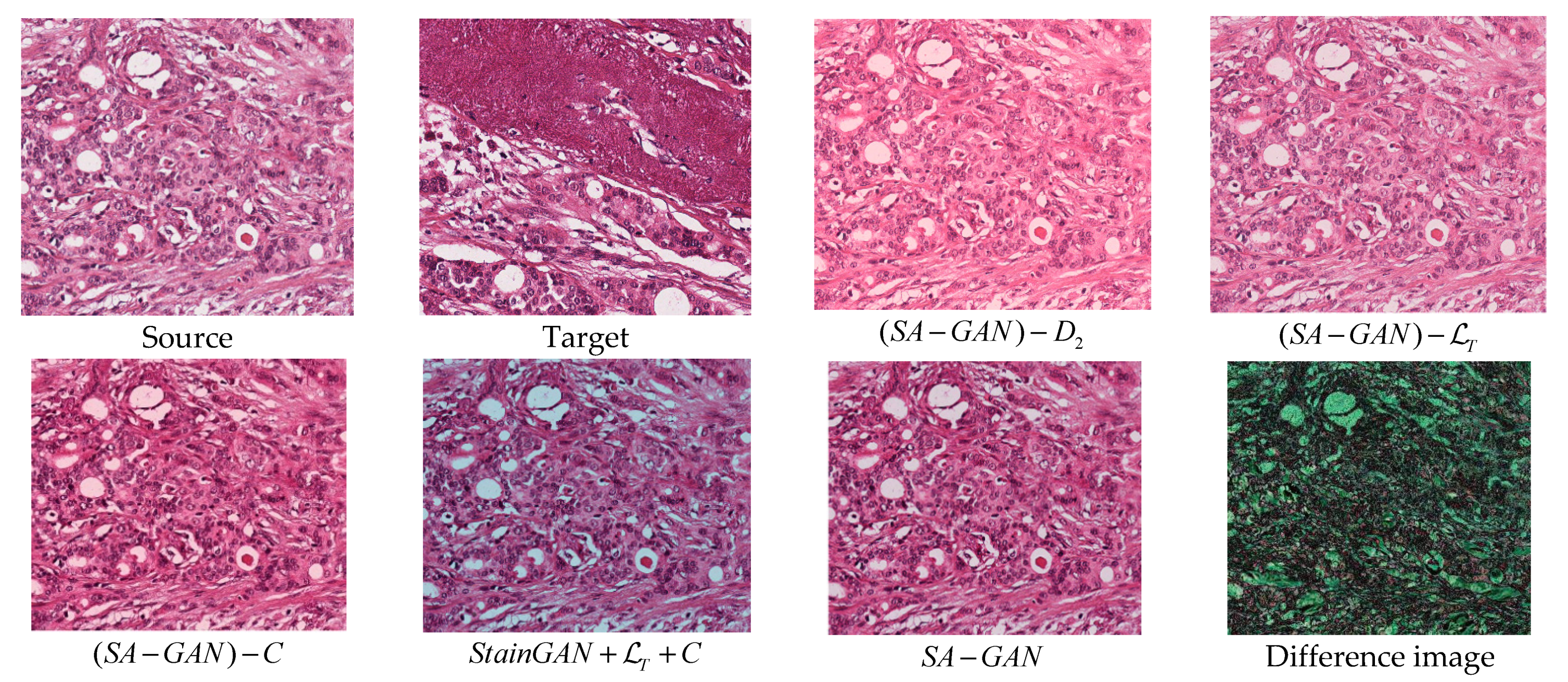
4.3. Ablation Experiments

The normalization performance is influenced by the architecture of the generative adversarial network model [27]. Recall that the architecture of SA-GAN consists of one generator and two discriminators which are trained by three different losses ${ℒ}_{D1}$, ${ℒ}_{D2}$, and ${ℒ}_T$. However, the question arises, as to why we need two discriminators instead of one. Is the structural loss ${ℒ}_T$ important? Is the color attribute metric necessary to maintain color contents in generated images? What will be the possible results if we combine the structural loss ${ℒ}_T$ and color attribute metric with other GAN structures such as StainGAN? To address these queries, ablation experiments are conducted. The CV-NMI and CV-NMH for different configurations of the proposed SA-GAN are shown in

Table 4. CV-NMI and CV-NMH for different configurations of the SA-GAN model.

	MITOS-ATYPIA-14		TUPAC 2016		ICIAR 2018		MICCAI’16
	CV-NMI	CV-NMH	CV-NMI	CV-NMH	CV-NMI	CV-NMH	CV-NMI	CV-NMH
No normalization	0.311	0.214	0.347	0.312	0.332	0.314	0.213	0.233
$(SA-GAN)-D_2$	0.018	0.019	0.025	0.020	0.018	0.017	0.016	0.025
$(SA-GAN)-{ℒ}_T$	0.017	0.020	0.024	0.022	0.016	0.018	0.018	0.020
$(SA-GAN)-C$	0.013	0.019	0.021	0.020	0.012	0.010	0.016	0.022
$StainGAN+{ℒ}_T+C$	0.133	0.122	0.119	0.099	0.123	0.117	0.116	0.123
$\mathrm{Proposed} SA-GAN$	0.012	0.017	0.021	0.018	0.011	0.010	0.014	0.021

. The following four configurations are designed for comparison.

(i) $(SA-GAN)-D_2$ represents the configuration without second discriminator D₂, (ii) $(SA-GAN)-{ℒ}_T$ is configuration when SA-GAN is trained without involving structural loss ${ℒ}_T$, (iii) $(SA-GAN)-C$ is configuration when SA-GAN is trained without color attribute metric constraint, and (iv) $StainGAN+{ℒ}_T+C$ is configuration when StainGAN [28] is trained with structural loss and color attribute metric.

As reflected from quantitative results (Table 4), the first four configurations poorly performed the color normalization. To further investigate, the effect of network architecture sample results for different settings of the design are given in Figure 6. As per results, the use of dual discriminators with adversarial losses is important and can achieve a desirable normalization consistency. Two discriminators deal with structure preserving and color transferring properties. It is important to note that color attribute constraint information assists the model in properly adjusting the colors from source domain to target domain. However, there is no substantial difference in metrics values, even when we exclude the color attribute information (Table 4 and Figure 6). This analysis proves that the proposed SA-GAN shows small sensitivity towards single target image in contrast to other color mapping methods [16,17,20,26]. It does not just rely on a single target image, rather involves the color distribution of whole dataset. Meanwhile, structure loss is also necessary to train the generator that is consistent with the results. Color distributions of test images obtained with SA-GAN are better matched with training images. On the other hand, the configuration of $StainGAN+{ℒ}_T+C$ does not preserve the structure details of source images in processed images. In general, the generator generates the images by obeying the distribution of target domain to make fool the discriminator. In histopathology, the distributions of structural contents and semantic colors in source domain and target domain are quite different. The single discriminator in StainGan has been misled to distinguish between generated image ${\widehat{x}}_S^n$ and target image $x_T^n$, causing loss of structure details. The proposed SA-GAN maintains the structure details in processed images and achieves a consistent normalization performance.

We did not perceive any performance improvement by changing α = 1 in Equation (6), whereas changing β = 1 and γ = 1 lead to a significant improvement of 10% in the CVs value.

4.4. Intra Dataset (Train and Test) Color Consistency Analysis

In this section, we quantify the impact of proposed SA-GAN on intra color variations that occur in the dataset obtained from a single laboratory (between training and test sets). To assess distribution similarity between train and test images, we computed histograms in Lab color space. Histograms of original and normalized images from test dataset are compared with training dataset. We measured the difference between histograms in terms of average histogram correlation (Corr) [40] and the Bhattacharyya distance (Dist_Bhat) [41]. The measured results are reported in

Table 5. Train-Test datasets color consistency analysis in terms of histogram correlation and Bhattacharyya distance using the proposed technique with other state-of-the-art methods.

	MITOS-ATYPIA-14		TUPAC 2016		ICIAR 2018		MICCAI’16
	$Corr$ ↑	$Dist\_Bhat$ ↓	$Corr$ ↑	$Dist\_Bhat$ ↓	$Corr$ ↑	$Dist\_Bhat$ ↓	$Corr$ ↑	$Dist\_Bhat$ ↓
Train-Test	0.101	0.813	0.098	0.830	0.121	0.867	0.110	0.820
Train-NormTest-SCD	0.231	0.615	0.211	0.601	0.122	0.667	0.202	0.570
Train-NormTest-Macenko	0.321	0.598	0.310	0.521	0.223	0.571	0.220	0.541
Train-NormTest-ACD	0.329	0.498	0.311	0.587	0.310	0.581	0.310	0.613
Train-NormTest-Reinhard	0.412	0.408	0.347	0.488	0.300	0.511	0.247	0.629
Train-NormTest-StainGan	0.428	0.380	0.337	0.476	0.330	0.455	0.341	0.521
Train-NormTest-SCAN	0.410	0.420	0.339	0.398	0.371	0.361	0.332	0.421
Train- NormTest-Proposed model	0.612	0.208	0.597	0.236	0.520	0.211	0.586	0.319

. A higher Corr and lower Dist_Bhat indicates that there is more similarity in color distributions of normalized datasets. Mathematically expressed as:

$$Corr=\frac{{\displaystyle \sum _m{\displaystyle \sum _n(}}{X}_{mn}-\overline{X})(Y_{mn}-\overline{Y})}{\sqrt{\left({\displaystyle \sum _m{\displaystyle \sum _n(}}{X}_{mn}-\overline{X}{)}^2\right)\left({\displaystyle \sum _m{\displaystyle \sum _n(}}{Y}_{mn}-\overline{Y}{)}^2\right)}}$$

(12)

$$Dist\_Bhat=\sqrt{1-\frac{1}{\sqrt{\overline{X}\overline{Y}{N}^2}}{\displaystyle \sum _m{\displaystyle \sum _n\sqrt{XY}}}}$$

(13)

where X and $Y$ represent the histograms of train and test images, respectively. $\overline{X}$ and $\overline{Y}$ denotes the mean value of histograms of X and $Y$, respectively.

As noted from the results, a low value of Corr and higher Dist_Bhat is obtained between the histogram of train and original test images. The high values of Dist_Bhat computed between train and original test data indicate larger differences in distributions, which can lead to poor generalization of deep CNN models. Our strategy obtained the highest correlation and lowest Bhattacharyya distance, improved without the color normalization (Table 5). SA-GAN accurately learns to transform the domain of source images (training images) to the domain of target images (test). The performance of proposed algorithm is also compared with state-of-the-art methods. Our proposed technique outperforms other color mapping algorithms [16,17,20,23,26], which confirms the advantage of structural loss ${ℒ}_T$ to maintain the structural contents in processed images (see Table 5).

4.5. Evaluation by Classification

Ultimately the effect of stain color normalization of histopathology images on the CAD system has been checked. Recently, several studies have utilized convolutional neural networks (CNNs) for histological image analysis [11,43,44]. Literature also shows that stain color normalization of histological images can increase the performance of deep CNN models [44,45,46]. We conducted this experiment to assess the significance of stain normalization methods for CNN based classification model. In this analysis, multiclass breast histology image classification were performed. We adopted the deep Resnet50 [30] image classification model and applied variational dropout [47]. At inference time, for each tested image, the model predicts the class probabilities and also provides a measure of uncertainty. The classification model differentiates breast histology images into four classes: Normal, Benign, In situ, and Invasive carcinoma. For this experiment, we divided the 400 training images into validation (100 images) and training (300 images) sets. For this experiment, we treated the validation data as an unseen test set. The small patches of 224 × 224 pixels were extracted from 2048 × 1536 pixels HPF images using a step size of 30 pixels. In the patch extraction process, about 24,000 patches were generated from 300 training images. The ResNet model [30] was separately trained on patches generated from original set of images and images processed by stain normalization methods [16,17,20,23,26,28].

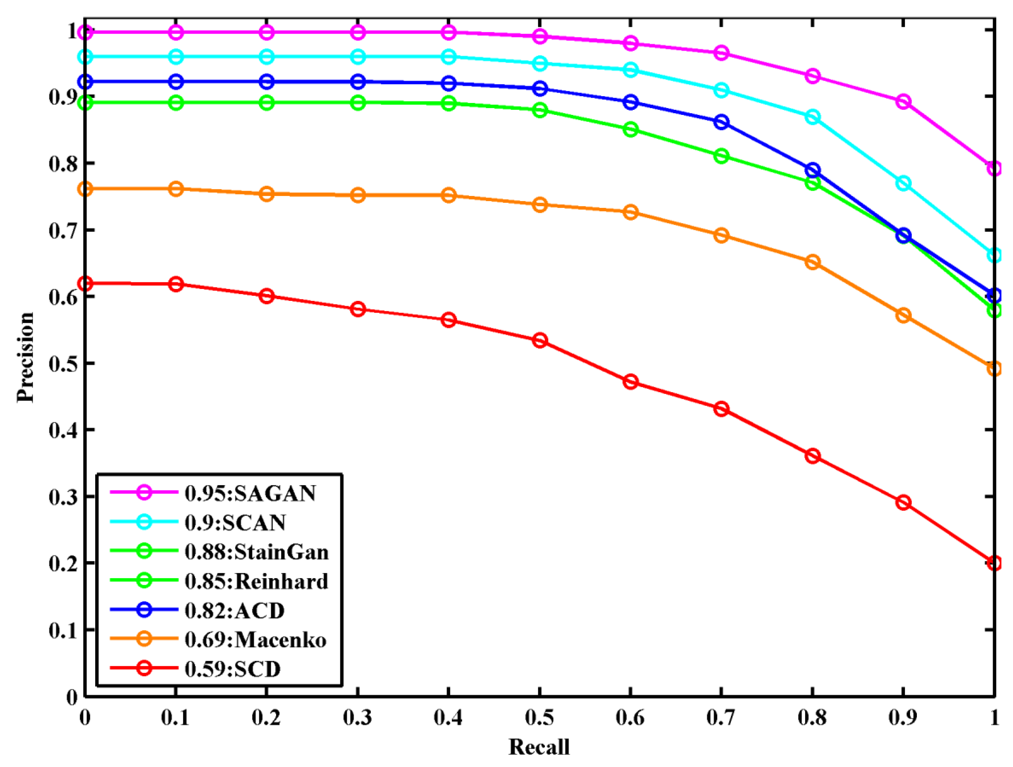
The precision–recall curve of the ResNet classification model to compare color normalization methods [16,17,20,23,26,28] on the validation dataset is shown in Figure 7. The classification model achieves the best detection results on stain normalized images obtained with the SA-GAN model compared to the normalized images by other methods, showing a 5.5% improvement on this part of data. In comparison to state-of-the-art normalization methods [16,17,20,23,26,28], our method effectively maintains the structural and color details of normalized images and provides benefits to achieve robust performance in the classification of histological images.

Classification performance on hidden test data: The class labels of the ICIAR test dataset are not publicly available (hidden by the challenge organizers). Therefore, detection results obtained with test data normalized by SA-GAN are submitted to organizers of BACH (https://iciar2018-challenge.grand-challenge.org) challenge for evaluation. The highest multiclass classification accuracy of 93% is achieved on the stain normalized (by SA-GAN) test images. The classification accuracy comparison with the ICIAR-2018 state-of-the-art methods (reported in [34]) on the hidden test dataset is given in

Table 6. Comparison of classification performance with ICIAR-2018 state-of-the-art on hidden test data (normalized by SA-GAN model).

Methods	Accuracy	Methods	Accuracy	Methods	Accuracy
Proposed model	0.93	Wang et al. [34]	0.83	Cao et al. [34]	79
Chennamsetty et al. [34]	0.87	Steinfeldt et al. [34]	0.81	Seo et al. [34]	79
Kwok [34]	0.87	Kone et al. [34]	0.81	Sidhom et al. [34]	78
Brancati et al. [34]	0.86	Nedjar et al. [34]	0.81	Guo et al. [34]	77
Marami et al. [34]	0.84	Ravi et al. [34]	0.80	Ranjan et al. [34]	77
Kohl et al. [34]	0.83	Wang et al. [34]	0.79	Mahbod et al. [34]	77

. The proposed design considerably improves the analysis outcome, showing a 6.9% improvement in accuracy on ICIAR 2018 hidden test data. The classification results (Table 6) confirm the advantages of the SA-GAN model to obtain the robust performance of CAD systems.

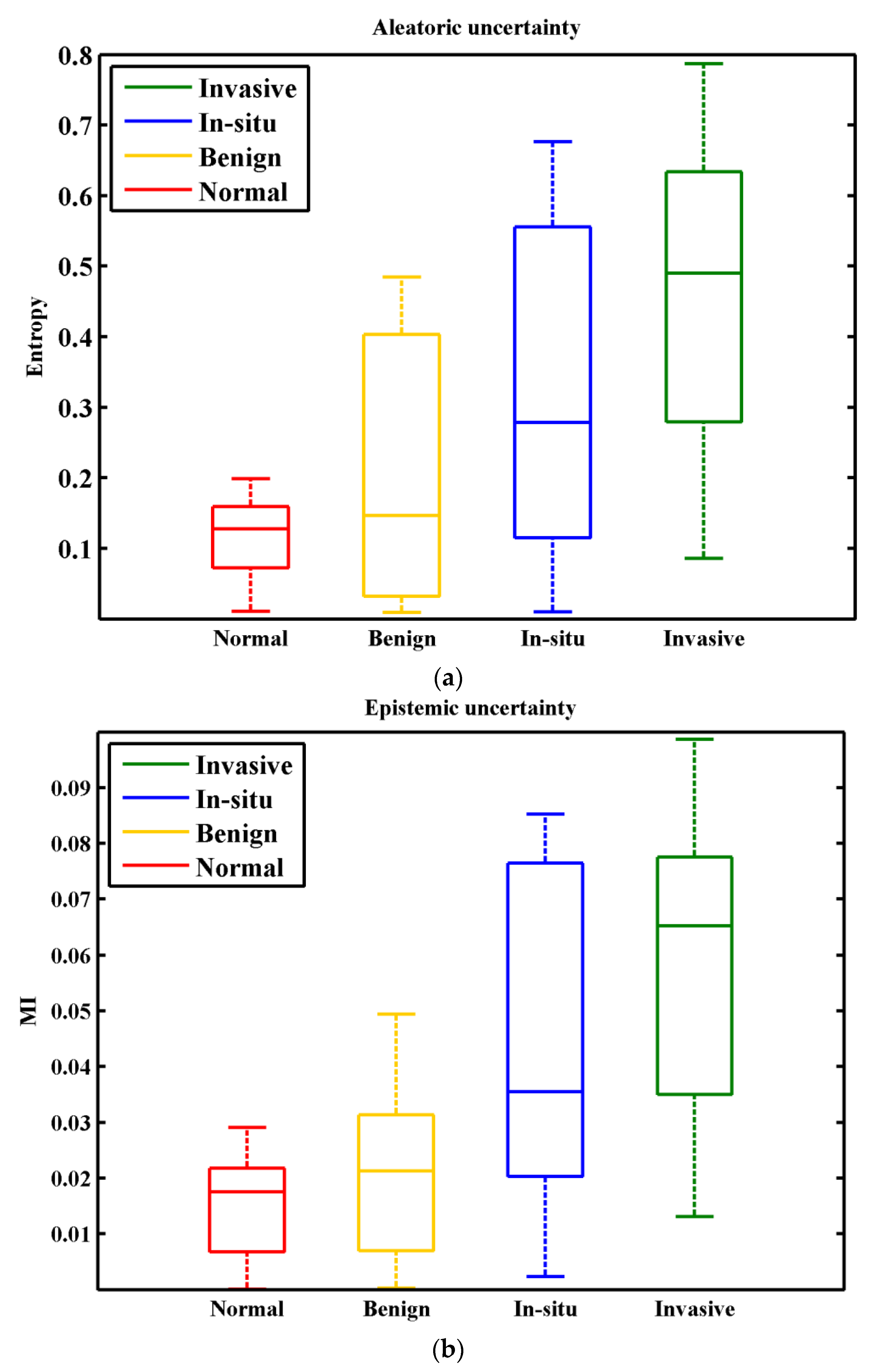
4.6. Uncertainty Estimation in Classification

To compute the uncertainty of predictions, two uncertainty measures: entropy H and mutual information MI are used [48]. It is believed that entropy and mutual information (MI) [48] measures the Aleatoric and Epistemic uncertainties [49] of model, respectively. The entropy of the perditions is defined as:

$$H\left[p\left(y|o,D\right)\right]=-{\displaystyle \sum _{y\in Y}p\left(y|o,D\right)\log p\left(y|o,D\right)}$$

(14)

where $p\left(y|o,D\right)$ is output conditional probability distribution of a model. If we obtain a label y for new input observation o by giving training dataset D, can be defined as:

$$MI\left(w,y|D,o\right)=H\left[p\left(y|o,D\right)\right]-{\mathbb{E}}_{p(w|D)}H\left[p\left(y|o,w\right)\right]$$

(15)

w in Equation (15) represents the amount of information that we gain about the model parameters. The MI denotes the difference between entropy of the predictions and the mean entropy of predictions. For uncertainty analysis, the performance of trained ResNet50 model is checked on validation set (100 images). We accounted multi class classification accuracy and uncertainty for each input image. The results for accuracy, entropy H, and mutual information MI, are shown in Figure 7 and Figure 8ab, respectively. Results show that the model obtained an average accuracy of 0.95 (Figure 7), entropy of 0.27, and MI of 0.035. From entropy analysis (Figure 8a), it can be seen that highest uncertainty values are recorded for the n situ carcinoma class. It is because similar structure statistics are repeated in inter-class images (i.e., In situ carcinoma and Invasive carcinoma classes). The results for MI are given in Figure 8b. Interestingly, according to MI more variance is present in the Begin class. However, the In situ class is relatively more certain in this case than in the entropy case. In multiclass classification, highest uncertainties values are recorded for inter-class images that have similar structure statistics. High uncertainty is an indicator of faulty class, capture the fact that misclassification mainly occurred for such inter-class images, we consider such images the bewildered images. It is important to notice that misdiagnosis of a cancer case is much worse than an unnecessary biopsy. So, the pathologist should re-examine such types of bewildered images before labeling them as non-invasive cancer.

5. Conclusions

Possible color inconsistencies and their implications in histopathology images have become a critical issue. Various stain normalization techniques have been proposed to condense the tissue inconsistencies. These techniques are paramount to accurate histopathology image analysis systems and guide the pathologists in their visual diagnostics. Normalization techniques have been used under the assumption that training and test sets of a dataset are of the same style characteristics. However, appearance variations in stained histopathology images originating from different pathology centers violate the above assumption. The main objective of color normalization process is to match the color patterns of the source and target domains images for the cancer classification task.

In this paper, we considered the color patterns of images as style patterns and carried out color transfer across the datasets. We designed a novel fully trainable framework named stain acclimation generative adversarial network (SA-GAN) that consists of one generator and two discriminators trained with two adversarial losses and one textural loss. The generator generates the images by obeying the distribution of the target domain. The discriminators enforce the generated images to modify color patterns and structure contents. In model training, color attribute metric helps the model to correctly learn the image-specific color patterns. The designed model performed an efficient mapping between the data domains by involving entire domain distribution and not altering the tissue structure of images. The empirical evaluations on four different histology datasets reveal the consistent normalization performance of proposed SA-GAN in comparison to state-of-the-art methods. The colors and contrast are exactly preserved in the processed images, which is most desirable for any color normalization method. The potential contribution of the proposed algorithm can be perceived collectively from efficient color normalization results, and improved classification performance for histopathology.