
Quantitative Geochemical Prediction from Spectral Measurements and Its Application to Spatially Dispersed Spectral Data


Abstract
:Featured Application
Abstract
1. Introduction
2. Materials
3. Methods
3.1. NMF
3.2. RFR
- Set any spectral reflectance values that are less than zero to zero (potential measurement errors). This is a requirement since the NMF cannot work with negative inputs;
- Transform the N × 1476 (1476 being the total number of spectral bands) individual spectra via the precomputed NMF model to the N × 25 sample space, where N is the number of spectral samples;
- Input the N × 25 NMF transformed spectra into the trained RFR model as input features and retrieve the estimated parameter values for Fe, SiO2, Al2O3, TiO, CaO, MgO, K2O and LOI.
4. Results
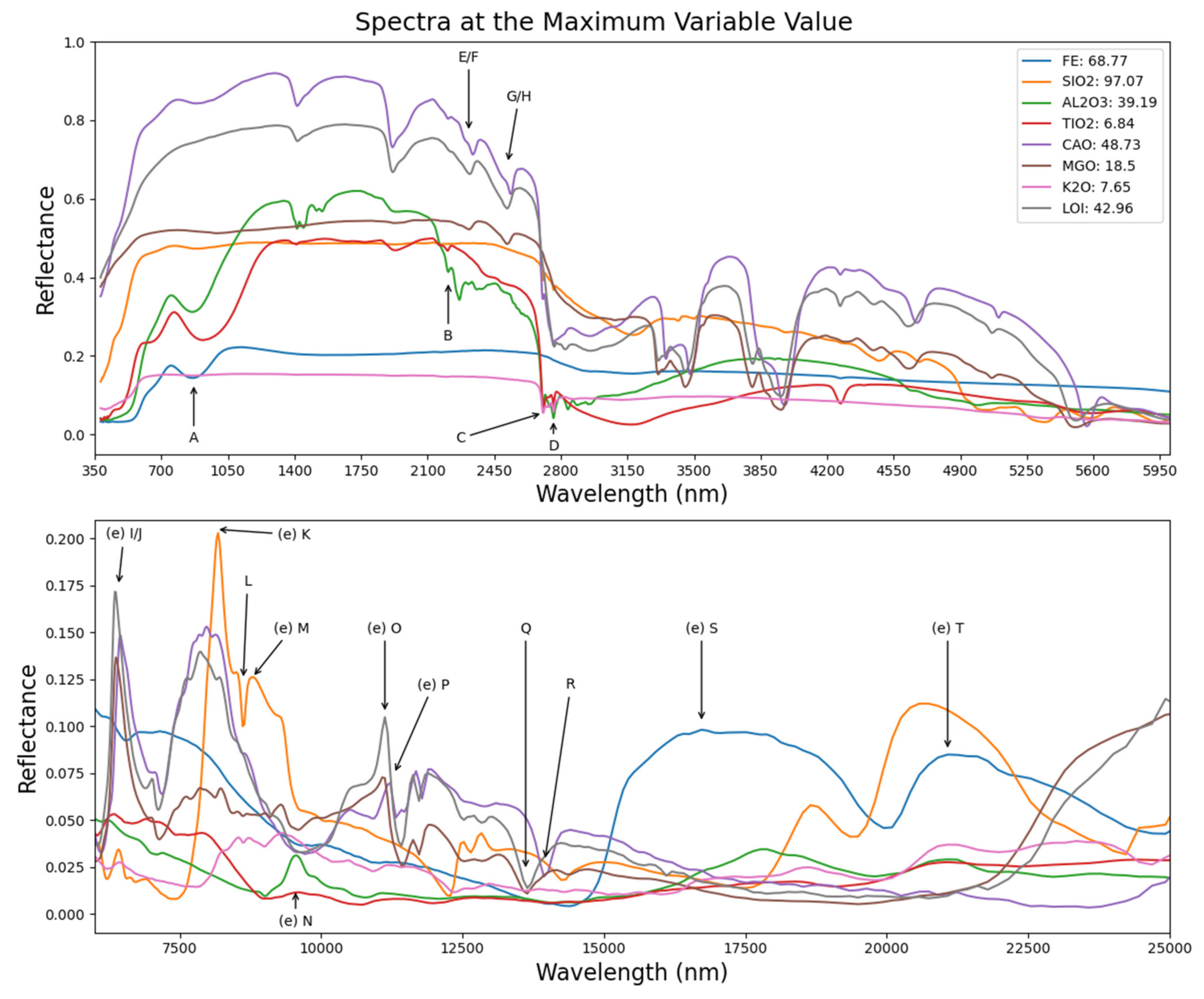
4.1. Spectral
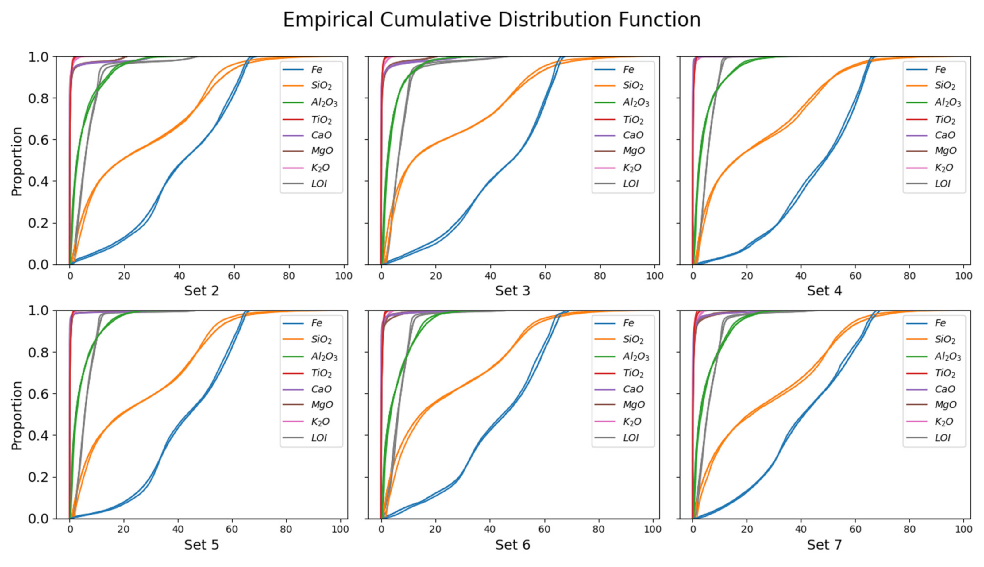
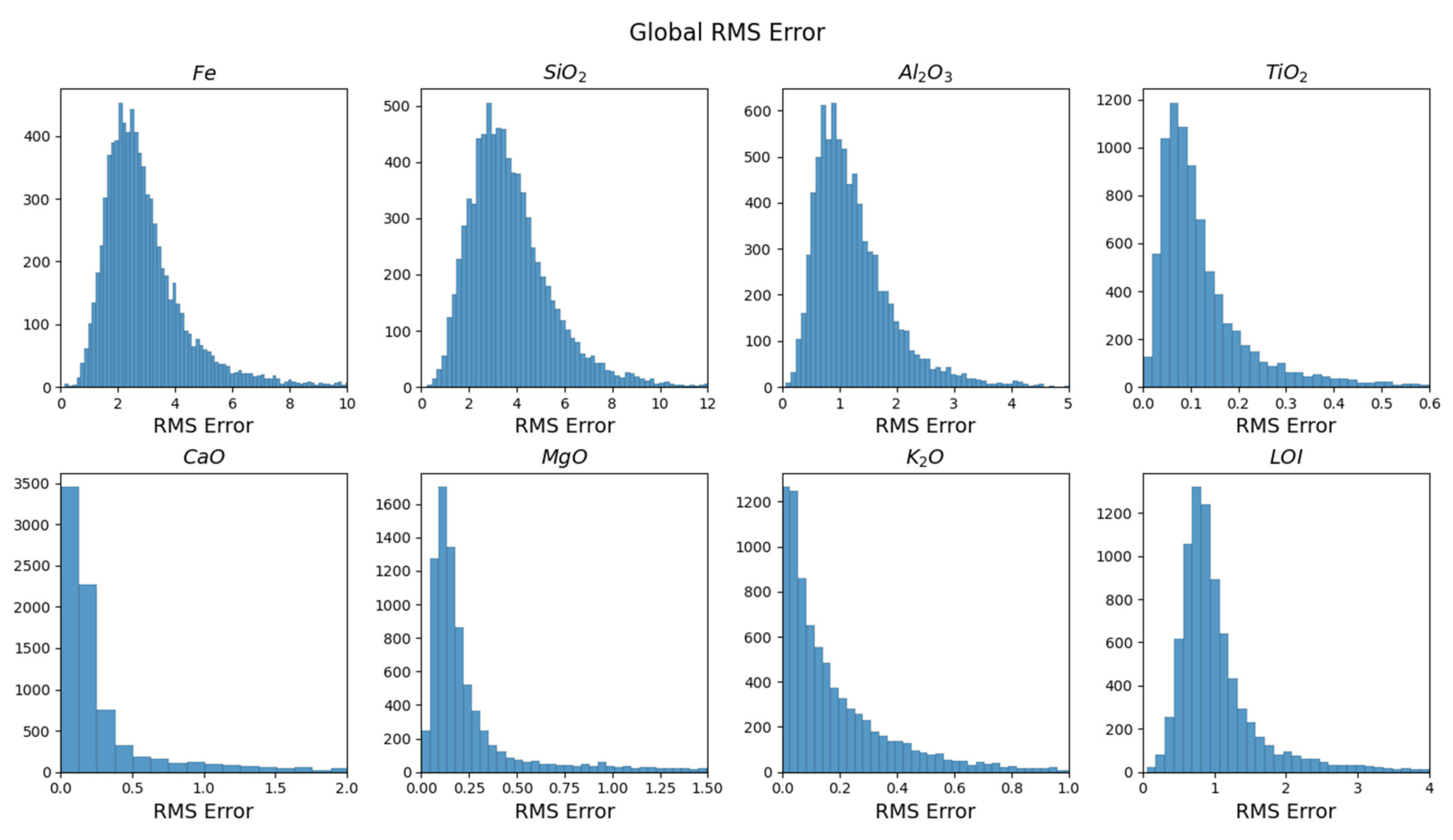
4.2. Global
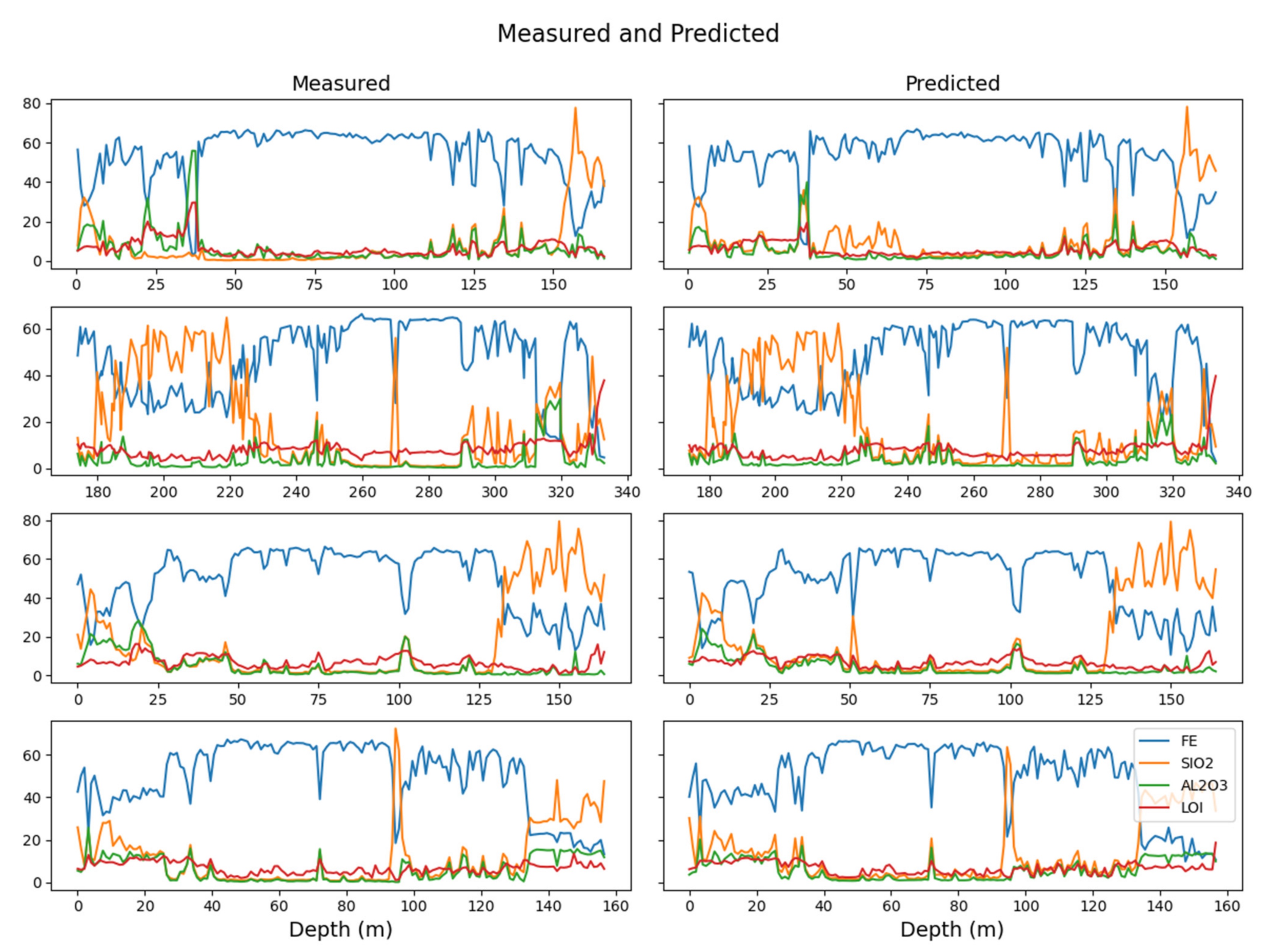
4.3. Downhole
5. Discussion
6. Conclusions
Author Contributions
Funding
Data Availability Statement
Conflicts of Interest
References
- Yamaguchi, Y.; Naito, C. Spectral Indices for Lithologic Discrimination and Mapping by Using the ASTER SWIR Bands. Int. J. Remote Sens. 2003, 24, 4311–4323. [Google Scholar] [CrossRef]
- Duke, E.F. Near Infrared Spectra of Muscovite, Tschermak Substitution, and Metamorphic Reaction Progress: Implications for Remote Sensing. Geology 1994, 22, 621–624. [Google Scholar] [CrossRef]
- Hewson, R.D.; Cudahy, T.J.; Caccetta, M.; Rodger, A.; Jones, M.; Ong, C. Advances in Hyperspectral Processing for Province-and Continental-Wide Mineral Mapping. In Proceedings of the 2009 IEEE International Geoscience and Remote Sensing Symposium, Cape Town, South Africa, 12–17 July 2009; Volume 4, p. IV-701. [Google Scholar]
- Cudahy, T.; Jones, M.; Thomas, M.; Laukamp, C.; Caccetta, M.; Hewson, R.; Verrall, M.; Hacket, A.; Rodger, A. Mineral Mapping Queensland: Iron Oxide Copper Gold (IOCG) Mineral System Case History, Starra, Mount Isa Inlier; Australasian Institute of Mining and Metallurgy: Gold Coast, QLD, Australia, 2008; pp. 153–160. [Google Scholar]
- Cudahy, T.; Jones, M.; Thomas, M.; Laukamp, C.; Caccetta, M.; Hewson, R.; Rodger, A.; Verrall, M. Next Generation Mineral Mapping: Queensland Airborne HyMap and Satellite ASTER Surveys 2006–2008; Commonwealth Scientific Industrial Research Organisation: Perth, Auatralia, 2008; p. 152. [Google Scholar]
- Wells, M.; Laukamp, C.; Hancock, E. Reflectance Spectroscopic Characterisation of Mineral Alteration Footprints Associated with Sediment-Hosted Gold Mineralisation at Mt Olympus (Ashburton Basin, Western Australia). Aust. J. Earth Sci. 2016, 63, 987–1002. [Google Scholar] [CrossRef]
- Green, D.; Schodlok, M. Characterisation of Carbonate Minerals from Hyperspectral TIR Scanning Using Features at 14,000 and 11,300 Nm. Aust. J. Earth Sci. 2016, 63, 951–957. [Google Scholar]
- Laukamp, C.; Cudahy, T.; Thomas, M.; Jones, M.; Cleverley, J.S.; Oliver, N.H.S. Hydrothermal Mineral Alteration Patterns in the Mount Isa Inlier Revealed by Airborne Hyperspectral Data. Aust. J. Earth Sci. 2011, 58, 917–936. [Google Scholar] [CrossRef]
- Laukamp, C.; Termin, K.A.; Pejcic, B.; Haest, M.; Cudahy, T. Vibrational Spectroscopy of Calcic Amphiboles–Applications for Exploration and Mining. Eur. J. Mineral. 2012, 24, 863–878. [Google Scholar] [CrossRef]
- Haest, M.; Cudahy, T.; Laukamp, C.; Gregory, S. Quantitative Mineralogy from Infrared Spectroscopic Data. I. Validation of Mineral Abundance and Composition Scripts at the Rocklea Channel Iron Deposit in Western Australia. Econ. Geol. 2012, 107, 209–228. [Google Scholar] [CrossRef]
- Agar, B.; Coulter, D. Remote Sensing for Mineral Exploration–A Decade Perspective 1997–2007. In Proceedings of the Exploration: Fifth Decennial International Conference on Mineral Exploration, Toronto, ON, Canada, 9–12 September 2007; Volume 7, pp. 109–136. [Google Scholar]
- Roache, T.J.; Walshe, J.L.; Huntington, J.F.; Quigley, M.A.; Yang, K.; Bil, B.W.; Blake, K.L.; Hyvärinen, T. Epidote–Clinozoisite as a Hyperspectral Tool in Exploration for Archean Gold. Aust. J. Earth Sci. 2011, 58, 813–822. [Google Scholar] [CrossRef]
- Geladi, P.; Kowalski, B.R. Partial Least-Squares Regression: A Tutorial. Anal. Chim. Acta 1986, 185, 1–17. [Google Scholar] [CrossRef]
- Hecker, C.; Dilles, J.H.; van der Meijde, M.; van der Meer, F.D. Thermal Infrared Spectroscopy and Partial Least Squares Regression to Determine Mineral Modes of Granitoid Rocks. Geochem. Geophys. Geosystems 2012, 13, 1–15. [Google Scholar] [CrossRef] [Green Version]
- Kun, W.; Keyan, X.; Nan, L.; Yuan, C.; Shengmiao, L. Application of Partial Least Squares Regression for Identifying Multivariate Geochemical Anomalies in Stream Sediment Data from Northwestern Hunan, China. Geochem. Explor. Environ. Anal. 2017, 17, 217–230. [Google Scholar] [CrossRef]
- Haaland, D.M.; Thomas, E.V. Partial Least-Squares Methods for Spectral Analyses. 1. Relation to Other Quantitative Calibration Methods and the Extraction of Qualitative Information. Anal. Chem. 1988, 60, 1193–1202. [Google Scholar] [CrossRef]
- Ritz, M.; Vaculikova, L.; Plevová, E.; Matỳsek, D.; Mališ, J. Determination of Chlorite, Muscovite, Albite and Quartz in Claystones and Clay Shales by Infrared Spectroscopy and Partial Least-Squares Regression. Acta Geodyn. Geomater. 2012, 9, 511–520. [Google Scholar]
- Breiman, L. Random Forests. Mach. Learn. 2001, 1, 5–32. [Google Scholar] [CrossRef] [Green Version]
- Kuhn, S.; Cracknell, M.J.; Reading, A.M. Lithologic Mapping Using Random Forests Applied to Geophysical and Remote-Sensing Data: A Demonstration Study from the Eastern Goldfields of Australia. Geophysics 2018, 83, B183–B193. [Google Scholar] [CrossRef]
- Kumar, A.S.; Keerthi, V.; Manjunath, A.S.; van der Werff, H.; van der Meer, F. Hyperspectral Image Classification by a Variable Interval Spectral Average and Spectral Curve Matching Combined Algorithm. Int. J. Appl. Earth Obs. Geoinf. 2010, 12, 261–269. [Google Scholar] [CrossRef]
- McKay, G.; Harris, J.R. Comparison of the Data-Driven Random Forests Model and a Knowledge-Driven Method for Mineral Prospectivity Mapping: A Case Study for Gold Deposits Around the Huritz Group and Nueltin Suite, Nunavut, Canada. Nat. Resour. Res. 2016, 25, 125–143. [Google Scholar] [CrossRef]
- Kirkwood, C.; Cave, M.; Beamish, D.; Grebby, S.; Ferreira, A. A Machine Learning Approach to Geochemical Mapping. J. Geochem. Explor. 2016, 167, 49–61. [Google Scholar] [CrossRef] [Green Version]
- Tuşa, L.; Khodadadzadeh, M.; Contreras, C.; Rafiezadeh Shahi, K.; Fuchs, M.; Gloaguen, R.; Gutzmer, J. Drill-Core Mineral Abundance Estimation Using Hyperspectral and High-Resolution Mineralogical Data. Remote Sens. 2020, 12, 1218. [Google Scholar] [CrossRef] [Green Version]
- Smith, B.R.; Huntington, J.F. Drillhole report for CHDDH77, Pine Creek Orogen, Northern Territory: National Virtual Core Library NTGS Node: HyLogger 2–7. NT Geol. Surv. Record 2010, 9, 2–7. [Google Scholar]
- Schodlok, M.C.; Whitbourn, L.; Huntington, J.; Mason, P.; Green, A.; Berman, M.; Coward, D.; Connor, P.; Wright, W.; Jolivet, M. HyLogger-3, a Visible to Shortwave and Thermal Infrared Reflectance Spectrometer System for Drill Core Logging: Functional Description. Aust. J. Earth Sci. 2016, 63, 929–940. [Google Scholar]
- Cracknell, M.J.; Jansen, N.H. National Virtual Core Library HyLogging Data and Ni–Co Laterites: A Mineralogical Model for Resource Exploration, Extraction and Remediation. Aust. J. Earth Sci. 2016, 63, 1053–1067. [Google Scholar] [CrossRef]
- Lee, D.D.; Seung, H.S. Learning the Parts of Objects by Non-Negative Matrix Factorization. Nature 1999, 401, 788–791. [Google Scholar] [CrossRef]
- Pedregosa, F.; Varoquaux, G.; Gramfort, A.; Michel, V.; Thirion, B.; Grisel, O.; Blondel, M.; Prettenhofer, P.; Weiss, R.; Dubourg, V. Scikit-Learn: Machine Learning in Python. J. Mach. Learn. Res. 2011, 12, 2825–2830. [Google Scholar]
- Lee, D.D.; Seung, H.S. Algorithms for Non-Negative Matrix Factorization. In Advances in Neural Information Processing Systems 13; Leen, T.K., Dietterich, T.G., Tresp, V., Eds.; MIT Press: Denver, CO, USA, 2001; pp. 556–562. [Google Scholar]
- Cichocki, A.; Phan, A.-H. Fast Local Algorithms for Large Scale Nonnegative Matrix and Tensor Factorizations. IEICE Trans. Fundam. Electron. Commun. Comput. Sci. 2009, 92, 708–721. [Google Scholar] [CrossRef] [Green Version]
- Févotte, C.; Idier, J. Algorithms for Nonnegative Matrix Factorization with the β-Divergence. Neural Comput. 2011, 23, 2421–2456. [Google Scholar] [CrossRef]
- Du, B.; Wang, S.; Wang, N.; Zhang, L.; Tao, D.; Zhang, L. Hyperspectral Signal Unmixing Based on Constrained Non-Negative Matrix Factorization Approach. Neurocomputing 2016, 204, 153–161. [Google Scholar] [CrossRef]
- Liu, R.; Du, B.; Zhang, L. Hyperspectral Unmixing via Double Abundance Characteristics Constraints Based NMF. Remote Sens. 2016, 8, 464. [Google Scholar] [CrossRef] [Green Version]
- Hamza, A.B.; Brady, D.J. Reconstruction of Reflectance Spectra Using Robust Nonnegative Matrix Factorization. IEEE Trans. Signal Process. 2006, 54, 3637–3642. [Google Scholar] [CrossRef] [Green Version]
- Bao, W.; Li, Q.; Xin, L.; Qu, K. Hyperspectral Unmixing Algorithm Based on Nonnegative Matrix Factorization. In Proceedings of the 2016 IEEE International Geoscience and Remote Sensing Symposium (IGARSS), Beijing, China, 10–15 July 2016; pp. 6982–6985. [Google Scholar]
- Févotte, C.; Dobigeon, N. Nonlinear Hyperspectral Unmixing with Robust Nonnegative Matrix Factorization. IEEE Trans. Image Process. 2015, 24, 4810–4819. [Google Scholar] [CrossRef] [Green Version]
- Berry, M.W.; Browne, M.; Langville, A.N.; Pauca, V.P.; Plemmons, R.J. Algorithms and Applications for Approximate Nonnegative Matrix Factorization. Comput. Stat. Data Anal. 2007, 52, 155–173. [Google Scholar] [CrossRef] [Green Version]
- Probst, P.; Boulesteix, A.-L. To Tune or Not to Tune the Number of Trees in Random Forest. J. Mach. Learn. Res. 2017, 18, 6673–6690. [Google Scholar]
- Scheinost, A.C. Use and Limitations of Second-Derivative Diffuse Reflectance Spectroscopy in the Visible to Near-Infrared Range to Identify and Quantify Fe Oxide Minerals in Soils. Clays Clay Miner. 1998, 46, 528–536. [Google Scholar] [CrossRef]
- Frost, R.L.; Johansson, U. Combination Bands in the Infrared Spectroscopy of Kaolins—A DRIFT Spectroscopic Study. Clays Clay Miner. 1998, 46, 466–477. [Google Scholar] [CrossRef]
- Gaffey, S.J. Spectral Reflectance of Carbonate Minerals in the Visible and near Infrared (0.35–2.55 Microns); Calcite, Aragonite, and Dolomite. Am. Mineral. 1986, 71, 151–162. [Google Scholar]
- Spitzer, W.G.; Kleinman, D.A. Infrared Lattice Bands of Quartz. Phys. Rev. 1961, 121, 1324–1335. [Google Scholar] [CrossRef]
- Lippincott, E.R.; Van Valkenburg, A.; Weir, C.E.; Bunting, E. Infrared Studies on Polymorphs of Silicon Dioxide and Germanium Dioxide. J. Res. Natl. Bur. Stand. 1958, 61, 61–70. [Google Scholar] [CrossRef]
- Madejová, J.; Komadel, P. Baseline Studies of the Clay Minerals Society Source Clays: Infrared Methods. Clays Clay Miner. 2001, 49, 410–432. [Google Scholar] [CrossRef]
- Ruan, H.D.; Frost, R.L.; Kloprogge, J.T. Comparison of Raman Spectra in Characterizing Gibbsite, Bayerite, Diaspore and Boehmite. J. Raman Spectrosc. 2001, 32, 745–750. [Google Scholar] [CrossRef] [Green Version]
- Ramanaidou, E.R.; Wells, M.; Belton, D.X.; Verrall, M.; Ryan, C. Mineralogical and Microchemical Methods for the Characterization of High-Grade Banded Iron Formation-Derived Iron Ore; Hagemann, S., Rosière, C.A., Gutzmer, J., Beukes, N.J., Eds.; Banded Iron Formation-Related High-Grade Iron Ore; Society of Economic Geologists: Littleton, CO, USA, 2008; Volume 15, pp. 129–156. [Google Scholar]
- Ramanaidou, E.; Wells, M.; Lau, I.; Laukamp, C. 6-Characterization of Iron Ore by Visible and Infrared Reflectance and, Raman Spectroscopies. In Iron Ore; Lu, L., Ed.; Woodhead Publishing: Sawston, UK, 2015; pp. 191–228. ISBN 978-1-78242-156-6. [Google Scholar]
- Zaini, N.; Van der Meer, F.; Van der Werff, H. Effect of Grain Size and Mineral Mixing on Carbonate Absorption Features in the SWIR and TIR Wavelength Regions. Remote Sens. 2012, 4, 987–1003. [Google Scholar] [CrossRef] [Green Version]
- Rowlands, N.; Neville, R.A. Calcite and dolomite discrimination using airborne SWIR imaging spectrometer data. Proc. SPIE 1996, 2819, 36–45. [Google Scholar] [CrossRef]
- Zaini, N.; Van der Meer, F.; Van der Werff, H. Determination of Carbonate Rock Chemistry Using Laboratory-Based Hyperspectral Imagery. Remote Sens. 2014, 6, 4149–4172. [Google Scholar] [CrossRef] [Green Version]
- Bishop, J.L. The Visible and Infrared Spectral Properties of Jarosite and Alunite. Am. Mineral. 2005, 90, 1100–1107. [Google Scholar] [CrossRef]


| Dataset | Statistic | Fe | SiO2 | Al2O3 | TiO2 | CaO | MgO | K2O | LOI |
|---|---|---|---|---|---|---|---|---|---|
| Train/Val | mean | 41.70 | 24.53 | 4.94 | 0.23 | 1.31 | 1.05 | 0.24 | 7.34 |
| std | 18.67 | 21.91 | 5.98 | 0.39 | 5.17 | 3.46 | 0.73 | 7.44 | |
| 50% | 43.85 | 16.16 | 2.49 | 0.08 | 0.04 | 0.09 | 0.01 | 5.68 | |
| 75% | 58.74 | 44.53 | 6.48 | 0.27 | 0.09 | 0.25 | 0.05 | 8.74 | |
| max | 69.15 | 98.70 | 53.38 | 8.63 | 52.47 | 22.00 | 9.36 | 84.79 | |
| Set 2 | mean | 41.18 | 25.83 | 5.32 | 0.27 | 0.98 | 0.80 | 0.17 | 7.21 |
| std | 17.62 | 21.95 | 6.29 | 0.42 | 4.47 | 3.05 | 0.56 | 7.05 | |
| 50% | 41.74 | 18.93 | 2.71 | 0.09 | 0.04 | 0.08 | 0.01 | 5.63 | |
| 75% | 57.29 | 46.14 | 7.25 | 0.34 | 0.08 | 0.19 | 0.04 | 8.94 | |
| max | 69.29 | 96.51 | 55.92 | 10.10 | 39.70 | 21.50 | 12.10 | 73.82 | |
| Set 3 | mean | 43.68 | 22.92 | 4.08 | 0.19 | 0.99 | 0.81 | 0.17 | 7.64 |
| std | 17.66 | 22.33 | 4.92 | 0.33 | 4.25 | 2.75 | 0.56 | 6.33 | |
| 50% | 47.90 | 11.87 | 2.30 | 0.08 | 0.04 | 0.09 | 0.01 | 6.34 | |
| 75% | 59.18 | 42.94 | 5.14 | 0.20 | 0.09 | 0.22 | 0.04 | 9.21 | |
| max | 68.13 | 96.76 | 51.72 | 7.76 | 49.87 | 20.80 | 11.60 | 73.23 | |
| Set 4 | mean | 45.66 | 23.01 | 4.78 | 0.20 | 0.11 | 0.14 | 0.12 | 5.83 |
| std | 16.12 | 20.52 | 5.70 | 0.31 | 0.96 | 0.57 | 0.44 | 3.05 | |
| 50% | 48.99 | 15.94 | 2.50 | 0.08 | 0.03 | 0.06 | 0.01 | 5.36 | |
| 75% | 59.56 | 40.11 | 6.07 | 0.24 | 0.05 | 0.10 | 0.03 | 7.81 | |
| max | 68.77 | 97.65 | 39.19 | 6.84 | 48.73 | 18.50 | 7.65 | 42.96 | |
| Set 5 | mean | 43.36 | 25.37 | 4.57 | 0.22 | 0.34 | 0.32 | 0.13 | 6.44 |
| std | 15.68 | 21.05 | 5.42 | 0.33 | 2.68 | 1.76 | 0.41 | 4.61 | |
| 50% | 44.33 | 19.45 | 2.36 | 0.08 | 0.01 | 0.05 | 0.01 | 5.64 | |
| 75% | 57.46 | 44.26 | 6.29 | 0.29 | 0.03 | 0.11 | 0.03 | 8.43 | |
| max | 67.32 | 97.73 | 51.14 | 5.96 | 40.53 | 21.00 | 6.85 | 47.01 | |
| Set 6 | mean | 43.00 | 23.52 | 5.67 | 0.31 | 0.48 | 0.59 | 0.24 | 6.85 |
| std | 17.34 | 21.43 | 6.16 | 0.48 | 2.76 | 2.11 | 0.67 | 4.83 | |
| 50% | 45.74 | 14.59 | 3.15 | 0.12 | 0.02 | 0.06 | 0.01 | 6.10 | |
| 75% | 58.11 | 43.35 | 8.75 | 0.46 | 0.06 | 0.21 | 0.10 | 9.09 | |
| max | 69.49 | 96.89 | 51.29 | 25.20 | 42.55 | 20.70 | 6.49 | 46.89 | |
| Set 7 | mean | 41.25 | 26.53 | 5.32 | 0.28 | 0.56 | 0.71 | 0.28 | 6.41 |
| std | 17.46 | 21.85 | 6.14 | 0.45 | 2.96 | 2.29 | 0.74 | 5.33 | |
| 50% | 41.30 | 20.73 | 2.70 | 0.10 | 0.03 | 0.10 | 0.01 | 5.40 | |
| 75% | 56.80 | 46.11 | 7.82 | 0.36 | 0.09 | 0.34 | 0.08 | 8.80 | |
| max | 69.49 | 97.66 | 48.03 | 8.63 | 37.42 | 20.40 | 7.07 | 46.76 |
| Label | Dominant Mineral Group Component/Group | Assignment | Literature | nm/cm−1 |
|---|---|---|---|---|
| A | iron oxide/Hematite | Fe3+ CFA (6A1 > 4T1) | [39] | 877/11,403 |
| B | kaolin group/Kaolin | n + dAl2OHi | [40] | 2209/4527 |
| C | kaolin group/Kaolin | nAl2OHo | [40] | 2705/3697 |
| D | kaolin group/Kaolin | nAl2OHi | [40] | 2761/3622 |
| E | Mg-rich Calcium carbonate/Dolomite | 3ν3CO3 | [41] | 2312–2323/4325–4305 |
| F | Calcium carbonate/Calcite | 3ν3CO3 | [41] | 2340/4237 |
| G | Mg-rich Calcium carbonate/Dolomite | 2ν3 + ν1 | [41] | 2505–2518/3992–3971 |
| H | Calcium carbonate/Calcite | 2ν3 + ν1 | [41] | 2530–2541/3953–3935 |
| I | Mg-rich Calcium carbonate/Magnesite | “ν3 peak” CO3 | [7] | 6405/1561 |
| J | Calcium carbonate/Dolomite | “ν3 peak” CO3 | [7] | 6490/1541 |
| K | Quartz/Quartz | ν(Si-O-Si) | [42] | 8150/1227 |
| L | quartz/Quartz | ν(Si-O-Si) | [42] | 8598/1163 |
| M | Quartz/Vitreous Silica | ν(Si-O-Si) | [43] | 9025/1108 |
| N | kaolin group/Kaolin Group | νSi-O | [44] | 9891/1011 |
| O | Mg-rich Calcium carbonate/Magnesite | “ν2 peak” CO3 | [7] | 11,058/904 |
| P | Calcium carbonate/Dolomite | “ν2 peak” CO3 | [7] | 11,236/890 |
| Q | Mg-rich Calcium carbonate/Ankerite | “ν4 trough” CO3 | [7] | 13,656/732 |
| R | Calcium carbonate/Calcite | “ν4 trough” CO3 | [7] | 13,942/717 |
| S | iron oxide/Hematite | Fe-O lattice vibration | [45] | 16,393/610 |
| T | iron oxide/Hematite | Fe-O lattice vibration | [45] | 22,026/454 |
| Dataset | Fe | SiO2 | Al2O3 | TiO2 | CaO | MgO | K2O | LOI | |
|---|---|---|---|---|---|---|---|---|---|
| Train/Val: 1185 | R2 | 0.99 | 0.99 | 0.97 | 0.88 | 0.99 | 0.99 | 0.92 | 0.98 |
| Set 2: 1603 | 0.96 | 0.96 | 0.92 | 0.64 | 0.96 | 0.95 | 0.60 | 0.92 | |
| Set 3: 1292 | 0.95 | 0.96 | 0.91 | 0.63 | 0.88 | 0.91 | 0.64 | 0.90 | |
| Set 4: 1087 | 0.97 | 0.97 | 0.95 | 0.74 | 0.82 | 0.77 | 0.68 | 0.87 | |
| Set 5: 1620 | 0.95 | 0.96 | 0.93 | 0.74 | 0.94 | 0.94 | 0.62 | 0.94 | |
| Set 6: 1542 | 0.95 | 0.96 | 0.91 | 0.62 | 0.89 | 0.82 | 0.67 | 0.88 | |
| Set 7: 1070 | 0.94 | 0.95 | 0.92 | 0.70 | 0.85 | 0.81 | 0.67 | 0.89 | |
| Average | 0.95 | 0.96 | 0.92 | 0.68 | 0.89 | 0.87 | 0.65 | 0.90 | |
| Train/Val: 1185 | RMSE | 1.74 | 2.13 | 0.82 | 0.09 | 0.29 | 0.23 | 0.13 | 0.78 |
| Set 2: 1603 | 3.00 | 3.83 | 1.29 | 0.15 | 0.41 | 0.35 | 0.18 | 1.16 | |
| Set 3: 1292 | 3.21 | 3.84 | 1.25 | 0.13 | 0.74 | 0.55 | 0.25 | 1.42 | |
| Set 4: 1087 | 2.69 | 3.46 | 1.23 | 0.12 | 0.23 | 0.19 | 0.19 | 0.96 | |
| Set 5: 1620 | 2.88 | 3.74 | 1.15 | 0.12 | 0.27 | 0.23 | 0.15 | 0.95 | |
| Set 6: 1542 | 2.91 | 3.71 | 1.30 | 0.13 | 0.32 | 0.32 | 0.18 | 1.09 | |
| Set 7: 1070 | 3.38 | 4.05 | 1.41 | 0.16 | 0.53 | 0.47 | 0.29 | 1.24 | |
| Average | 3.01 | 3.77 | 1.27 | 0.13 | 0.41 | 0.35 | 0.21 | 1.14 | |
| Train/Val: 1185 | Sdev RMSE | 0.99 | 1.21 | 0.42 | 0.10 | 0.43 | 0.32 | 0.16 | 0.49 |
| Set 2: 1603 | 1.62 | 1.95 | 0.86 | 0.15 | 0.71 | 0.53 | 0.27 | 1.20 | |
| Set 3: 1292 | 2.01 | 1.99 | 0.71 | 0.14 | 1.36 | 0.69 | 0.27 | 1.39 | |
| Set 4: 1087 | 1.26 | 1.65 | 0.55 | 0.09 | 0.40 | 0.22 | 0.19 | 0.54 | |
| Set 5: 1620 | 1.68 | 1.86 | 0.68 | 0.11 | 0.51 | 0.31 | 0.16 | 0.56 | |
| Set 6: 1542 | 1.39 | 1.72 | 0.82 | 0.14 | 0.61 | 0.56 | 0.23 | 0.76 | |
| Set 7: 1070 | 1.93 | 1.95 | 0.84 | 0.16 | 0.78 | 0.66 | 0.29 | 0.92 | |
| Average | 1.65 | 1.85 | 0.74 | 0.13 | 0.73 | 0.49 | 0.24 | 0.89 |
Publisher’s Note: MDPI stays neutral with regard to jurisdictional claims in published maps and institutional affiliations. |
© 2021 by the authors. Licensee MDPI, Basel, Switzerland. This article is an open access article distributed under the terms and conditions of the Creative Commons Attribution (CC BY) license (https://creativecommons.org/licenses/by/4.0/).
Share and Cite
Rodger, A.; Laukamp, C. Quantitative Geochemical Prediction from Spectral Measurements and Its Application to Spatially Dispersed Spectral Data. Appl. Sci. 2022, 12, 282. https://doi.org/10.3390/app12010282
Rodger A, Laukamp C. Quantitative Geochemical Prediction from Spectral Measurements and Its Application to Spatially Dispersed Spectral Data. Applied Sciences. 2022; 12(1):282. https://doi.org/10.3390/app12010282
Chicago/Turabian StyleRodger, Andrew, and Carsten Laukamp. 2022. "Quantitative Geochemical Prediction from Spectral Measurements and Its Application to Spatially Dispersed Spectral Data" Applied Sciences 12, no. 1: 282. https://doi.org/10.3390/app12010282
APA StyleRodger, A., & Laukamp, C. (2022). Quantitative Geochemical Prediction from Spectral Measurements and Its Application to Spatially Dispersed Spectral Data. Applied Sciences, 12(1), 282. https://doi.org/10.3390/app12010282