Abstract
The detachment regime has a high potential to play an important role in fusion devices on the road to a fusion power plant. Complete power detachment has been observed several times during the experimental campaigns of the Wendelstein 7-X (W7-X) stellarator. Automatic observation and signaling of such events could help scientists to better understand these phenomena. With the growing discharge times in fusion devices, machine learning models and algorithms are a powerful tool to process the increasing amount of data. We investigate several classical supervised machine learning models to detect complete power detachment in the images captured by the Event Detection Intelligent Camera System (EDICAM) at the W7-X at each given image frame. In the dedicated detached state the plasma is stable despite its reduced contact with the machine walls and the radiation belt stays close to the separatrix, without exhibiting significant heat load onto the divertor. To decrease computational time and resources needed we propose certain pixel intensity profiles (or intensity values along lines) as the input to these models. After finding the profile that describes the images best in terms of detachment, we choose the best performing machine learning algorithm. It achieves an F1 score of 0.9836 on the training dataset and 0.9335 on the test set. Furthermore, we investigate its predictions in other scenarios, such as plasmas with substantially decreased minor radius and several magnetic configurations.
1. Introduction
The previous years brought a considerable increase in the different applications of machine learning in all fields of natural sciences and, in particular, in fusion plasma physics [1,2,3,4]. With the growing discharge times in fusion devices comes a growing amount of data that has to be processed. Machine learning is a powerful tool in the hands of physicists to be able to process and analyze this growing amount of data. As the first step to a (supervised) machine learning toolkit for fusion research, we trained several classical machine learning (ML) algorithms, to be able to detect plasma detachment in the images captured by the EDICAM camera system [5,6] in the Wendelstein 7-X stellarator [7,8,9,10]. One of the major aims of this study was to show that power detachment can be detected using the combination of the installed video diagnostics and intelligent algorithms, and how these algorithms can enhance the capabilities of such diagnostics.
Controlling the location where the plasma is in contact with the surrounding vacuum vessel is crucial in fusion devices. In a so-called divertor configuration, the magnetic field lines in the peripheral region, the scrape-off layer (SOL), are diverted towards dedicated targets, called plasma facing components (PFCs), which intersect the plasma. The surface in between the main plasma volume with closed magnetic field lines and the SOL is called separatrix. The main advantage of such configuration is that the plasma is only in contact with solid surfaces made for this exact purpose. However, this also leads to high concentration of the power flux in a narrow stripe along the line of the separatrix–divertor target intersection, called strike line [11]. Reduction of this significant power load is a must in future high-power fusion devices; a potential solution is achieving a regime called divertor detachment. We achieve detachment by density increase or by puffing additional gas—typically a lower-Z impurity, such as Nitrogen—in the divertor domain, resulting in a decrease of plasma ion flux, accompanied by a large drop of plasma density and temperature in the edge plasma region, in front of the targets. The consequence of these phenomena is the significant reduction of power load on the divertor tiles. Detachment can solve the problem of erosion and heat load on the PFCs, thus is considered to be the primary operating regime for ITER [12].
2. Methods
2.1. Experimental Setup
The Wendelstein 7-X (W7-X), based in Greifswald, Germany, is the largest stellarator type fusion device in the world, aiming at demonstrating the reactor relevance of optimized stellarators. The main objectives are achieving plasma discharges as long as 30 min and heating power of 10 MW. The first plasma was produced in 2015; the road to steady-state operation consists of various Operating Phases (OP) to gradually increase the machine performance, carry out experiments and test new ideas. For the first experimental runs (OP1.1) [13] it had a simple setup of plasma facing components, using 5 inertially cooled discrete graphite inboard limiters. In OP1.2 [14] a more expanded set of PFCs, including a test divertor, which already had the exact same shape as the water cooled divertor presently being installed, were installed enabling a significant increase in plasma density and heating power. Thanks to the new set of PFCs, feedback controlled divertor gas fuelling capability and a surface conditioning [15], the circumstances were satisfactory to reach complete power detachment in the device [11].
In order to facilitate smooth operation, W7-X is equipped with a wide variety of diagnostics. Video diagnostics, both infrared and visible, play a key role in the visualization of several different plasma phenomena and in the protection against dangerous plasma-wall interactions. The visible video diagnostics is seen in Figure 1, it is based on ten cameras in toroidally viewing “oblique equatorial” (AEQ) ports, covering 95% of the interior. Due to the thick cryostat vessel of the device, each camera is attached to the end of 2-meter-long, flexible tubes to be able to reach the inner end of the observational ports [5]. The so-called Event Detection Intelligent Cameras (EDICAMs) serve as the workhorse for the visible video diagnostics. The EDICAMs use a special 1.3 megapixel CMOS sensor with non-destructive read capability, enabling fast monitoring of smaller, predefined Regions of Interest (ROIs) in parallel to a normal, slow framing (100 Hz), full-frame overview [6]. The camera can perform simple operations on the ROI data in real-time, which can adapt and change the readout process and generate various output signals. The camera hardware has two main parts: the camera head, containing only the most necessary electronics including the sensor module, and the FPGA-based image processing and control unit (IPCU), mounted in a control PC as a PCIe extension card; these two components are connected via a 10 gigabit/s fiber link running through the previously mentioned flexible tube.
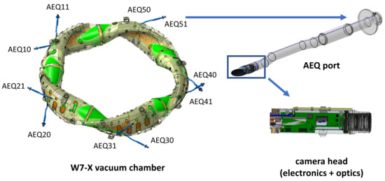
Figure 1.
Schematics of the video diagnostics system at the W7-X and the EDICAM.
Since the cameras are installed in a tangential observation geometry, they see the projected cross-sections of the 3-dimensional plasma. Under normal operational conditions the plasma emits visible radiation only at its edge, thus a slim radiation belt can be observed in the images. The shape of this radiation belt is not trivial: W7-X is based on a helias configuration, i.e., the plasma lacks axial symmetry; in other words, the poloidal cross-section of the plasma changes continuously when moving along the toroidal direction. Therefore, the observed radiation belt is the superposition of poloidal cross-sections at different toroidal locations within the camera’s view range. Even so, the changes in the size of the plasma—or more precisely, the location of visible light emission—can be observed surprisingly well by looking at the radiation belt.
2.2. Detachment Seen in the Images
In Figure 2. we may discover the following characteristics:
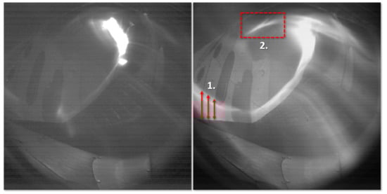
Figure 2.
Images of attached (left) and detached plasmas (right). The most distinctive differences are marked with red on the detached image: Increased distance between the inner wall and the radiation belt (1), a tail-like structure strengthening in the radiation belt (2).
- Overall growth of visible radiation during divertor detachment;
- Increased distance between the inner wall and the radiation belt (1);
- The strengthening and moving of a tail-like structure in the radiation belt (2).
These observations reinforced the hypothesis that detachment could be detected using computer vision solutions.
Our idea was to significantly reduce the amount of data to be processed by pre-selecting parts of the image where the effect of detachment is most pronounced. Following preliminary analyses, we decided to use as inputs up to 200 pixel intensity values along particular lines in the images, in other words pixel intensity profiles. Five regions were identified on the image, where the radiation belt shows a similar behavior within the regions but behaves differently in each of them. Region A (located at the outer wall): changes in the plasma size corresponds to a significant movement of the radiation pattern. Region B (inner wall): here the distance between the plasma and the wall can clearly be seen, although the radiation pattern moves much less when the plasma size changes. Region C (above divertor baffle): here a tail-like structure changes its position and intensity significantly when the plasma goes to detachment. Region D (divertor): the image is often overexposed here, therefore we exclude it from the analysis. Region E (outer wall/ports): no light emission is detected here. To appropriately capture the changes of the plasma, a homogeneous background was needed behind the radiation belt and along the profile, so we had to place them in such areas of the examined parts of the images. We selected three profiles in all three useful regions, A, B and C, as shown in Figure 3, to be qualified during a pre-selection test. We found that these profiles describe the images well with regards to detachment. Figure 3 shows the characteristics of profile A in a detached and a non-detached plasma. The increase in overall visible radiation is seen, along with the maximum point of the graph shifting towards the confined region, thus the distance between the stellarator wall and the radiation belt is increasing.
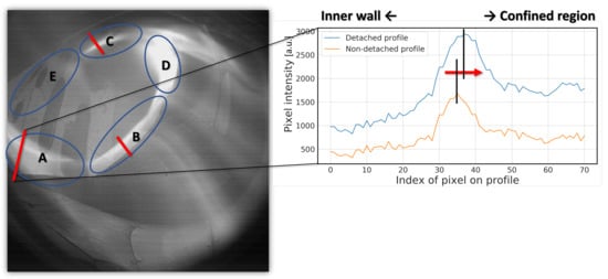
Figure 3.
The regions A, B, C, D and E indicated with blue ellipses in one image (left). Two examples for profile A (right); one detached (blue) and one non-detached (orange). The confined region in this case is in the direction of the increasing pixel indexes, we can see the maximums of the graphs shifting that way during detachment.
2.3. Models
During our work we looked at three classical supervised machine learning models, using the implementations found in the Sklearn Python library [16]. We presumed that the classical machine learning models need much less data and time of training to achieve a sufficient level of accuracy then advanced ones like neural networks, thus these algorithms are the primary focus of this paper.
The first and simplest classical classification algorithm is the Logistic Regression [17]. Despite its name it is a linear classification method. Using this model we fit the logistic function to the data to get the probabilities for a sample belonging to one of two classes. Sklearn’s implementation uses an L2 regularized version of this model as default, for further information we refer to [18].
The Support Vector Machine (SVM) [17] fits a separating hyperplane to the data, in such way that the model tries to find the hyperplane which has the maximal distance to the nearest data point, thus achieving good generalization ability.
The last classical supervised algorithm we used is the Random Forest [17]. It is among the most powerful and widely used statistical models. It is an ensemble of hierarchical data structures called decision trees, which are built from bootstrap samples of the training set. Individual decision trees typically exhibit high variance and tend to overfit, but combining their predictions using averaging makes the random forest a robust method.
2.4. The Dataset
An important experimentally measured indicator of detachment is the fraction of radiated power , which can be calculated as radiated power divided by the plasma heating power . As seen in [19], the most advanced simulations of the W7-X detachments predicts that when exceeds approximately 0.5, the radiation zone begins to detach from the target and starts to move inward; between 0.8 and 0.9 the temperature and the pressure on the last closed flux surface (in our case, the separatrix) falls drastically. Being aware of these results, we used as indicator for detachment and built our dataset accordingly.
Our dataset consists of images taken during the OP1.2 campaign in 2018, using the camera in the AEQ50 port (for the particular discharges we refer to Table 1). The dataset was divided into three parts: training data, validation data and test data. The training set is made of approximately 7770 images from 16 different discharges; from these, 3889 are detached and 3882 are non-detached. For the latter we found it important to contain a wide variety of images, e.g., plasma start-up, plasma end and non-detached images from discharges with and without a detachment phase. Besides that, three additional discharges were reserved. One, discharge 20181016.016, to serve as a validation dataset during the cross-validation process (for more detail see later), and two shots, 20180814.023 and 20181010.035, to calculate the performance metrics of the models (test). Both have detached intervals from 4.18 s to 7.84 s and from 2.89 s and to 6.75 s, respectively.

Table 1.
The discharges and their chosen intervals used for constructing the training dataset.
After gathering these images, we extracted the appropriate pixel intensity profiles (our workflow can be seen in Figure 4). We represent each profile as a vector, these vectors make up a matrix X. This matrix, paired up with a vector y containing binary values for each profile in the matrix, indicating if the profile is detached (1) or non-detached (0), are the inputs to the models.
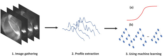
Figure 4.
Detachment detection workflow. 1. The EDICAM camera system takes images in the vessel. 2. We extract the appropriate intensity profiles from the images. 3. We use the profiles as inputs to a machine learning models to determine detachment or non-detachment. Greatly simplified schematics of the (a) Logistic Regression model (b) the Random Forest model.
The dataset was created while keeping in mind that we only want to decide if on the given image the fusion plasma is in a dedicated detached state or not. In the dedicated detached state the plasma is stable despite its reduced contact with the machine walls, filling up the available space in the vacuum chamber as much as possible, without exhibiting significant heat load onto the divertor. There are various other plasma states when the plasma is not in contact with the divertor either, and in which the radiation belt moves deeply inside the core plasma, far away from the separatrix. Technically, these states are also detached, but usually unstable—we aim to get a negative response from our algorithm for these states, hence we use the term “non-detached” instead of simply using “attached”.
2.5. Data Preprocessing
Scaling the data appropriately is an important step before feeding it to machine learning algorithms. Many algorithms (e.g., Support Vector Machines) assume that all features are centered around 0 and have unit variance. Therefore, standardizing the data by removing the mean and scaling to unit variance boosts the performance of these models significantly. Standardization happens independently on each feature. We used standardization on all our models.
2.6. Performance Evaluation Metrics
Several metrics can be used for measuring the performance of classification models. The first and foremost step to acquire these metrics is to calculate the confusion matrix of the predictions. Each row of the matrix represents the instances in a predicted class, while each column represents the instances in an actual class as seen in Figure 5.
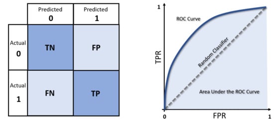
Figure 5.
Schematics of the confusion matrix (left). Schematics of the Reciever Operating Characteristic Curve (right). The meaning of the used abbreviations; TN: True Negative, FP: False Positive, FN: False Negative, TP: True Positive.
First we define Precision as and Recall as , by calculating the harmonic mean of these quantities we get the F1 score:
The F1 score takes into account how the data are distributed, thus is accurate for both balanced and unbalanced datasets. The Receiver Operating Characteristic Curve (ROC Curve) illustrates the performance of a binary classification model as its discrimination threshold is varied. We create the ROC curve by plotting the recall (or true positive rate—TPR) as a function of false positive rate (FPR), where , for each examined threshold value. By integrating the curve, we get the Area Under the ROC Curve (AUC) metric, which shows us the ability of the model of separating the two classes. AUC varies between 0 and 1, with a random classifier yielding 0.5.
3. Results
3.1. Best Profile
First, we evaluated the pre-selected profiles, i.e., we selected which pixel intensity profile to use throughout the work. To find the profile that describes detachment in the images best, we trained the three previously described classical models with default parameters on all the profiles separately. We calculated their TPR, , F1 scores and Area Under Curves metrics on the validation set, the result can be seen in Table 2.
Table 2.
TPR, , F1 and AUC scores of the models on the separate profiles. Ee indicated the highest score (or lowest for ) per model with bold and green text, if we had matching best values, we used only bold text.
It can be clearly seen that the models had the best performance using profile A, having the most number of highest metrics across the models.
3.2. Best Model
From this point we used data gathered from profile A on all our models. To find the most accurate model, we performed hyperparameter search using the grid search cross fold validation method. In machine- and deep learning the model specific parameters which are used to control the learning process are called hyperparameters, these are different from the previously mentioned weight parameters, because they cannot be modified while training. Some examples for hyperparameters are learning rate, the method of optimization algorithm, etc.
During grid search we define a range of hyperparameters, at each iteration we choose a random combination of such parameters, train the models on these using the training set, calculate their F1 score on a random subset of the validation set and in the end, after a given number of iterations, we adopt the best performing combinations for the models. The advantage of applying cross fold validation is that at each iteration we calculate the F1 scores on random subsets of a given validation set, thus testing the model’s performance on new data that was not seen before, we can avoid overfitting and see how the model generalizes to new independent data.
The results can be seen in Table 3. On the training set the logistic regression and the support vector machine models have the best performances, almost identical. However, when calculating the F1 scores on the previously not seen two discharges, the test dataset, the logistic regression by far beats the other two models.
Table 3.
The used models and their achieved performance metrics during training and test.
The predictions of the three models on one of the test shots, namely 20181010.035 is seen on Figure 6. From this we can identify where the logistic regression exactly beats the other models. The support vector machine and the random forest makes a lot more false positive predictions, particularly before the beginning of the detached interval. All three models perform well inside this interval, but they also have a common mistake.
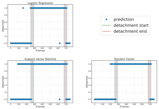
Figure 6.
Predictions of the various models on discharge number 20181010.035. The F1 scores are not determined in the transition zones.
We know that the transition to detachment takes place gradually, but we used binary indicators in our datasets, a consequence of such actions is that we cannot determine the exact point in time where the turnover to detachment takes place. Relying on our experiences gained while working with the dataset, we could establish there is a maximum of 40-frame-long “transition zone”, indicated with gray-shaded areas on the figures. It is important to note that the F1 scores were not calculated in these intervals.
Before performing the analysis of the models, our precondition was, that the final algorithm must have at least an F1 score of 0.9 on the test dataset. Since the logistic regression could only produce this number, that is the model we used going forward. For further analysis on the models performance we refer to Appendix A.
3.3. Performance in Other Magnetic Configurations, Small Plasmas
The experiments to achieve complete power detachment were using the standard (EJM) magnetic configuration [20], thus the majority of the discharges used for training had this magnetic configuration. To examine the generalization ability of our model, we had to explore the predictions on discharges with other magnetic configurations. The configurations investigated furthermore were the so-called high iota (FTM), high mirror ratio (KJM) and an other standard-like (EIM). Namely the discharges 20180822.009, 20181009.011 and 20180829.055. There was no detachment observed during these shots, we were interested if the model would make false positive predictions. The results are seen in Figure 7. Our model made almost no false positive predictions, predicted no detachment for the entirety of the discharges, rightly so. We can conclude, that the previously chosen best performing model is not tricked by seeing other magnetic configurations, thus having an understanding of detachment independent from the changes in them.
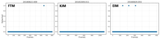
Figure 7.
Predictions on FTM, KJM and EIM magnetic configurations.
As stated previously in Section 2.4, we are interested in detecting a detached state where the plasma is stable, filling up the available space in the vacuum chamber as much as possible. During the various experimental runs of the Wendelstein 7-X several other detached states were observed, where the size of the plasma decreases extremely, so called “small plasmas” [21]. An example of such small plasma discharge is shown in Figure 8. As discussed before, having false positive predictions for these discharges would compromise the practicality of using such algorithm to detect detachment, so we had to make sure this does not happen. We ran predictions for several discharges with small plasmas and had a negligible false positive predictions.

Figure 8.
Examples of “small plasmas” observed in the W7-X during discharge 20171207.021 with the location of the intensity profile (i.e., the part of the image where data processing takes place).
4. Summary and Outlook
We presented our first step to a machine learning toolkit for fusion diagnostics developed by our research group. We found that power detachment in the Wendelstein 7-X stellarator can be detected using the combination of ML algorithms and video diagnostics, making the capabilities of such diagnostics more versatile. To decrease the amount of data that has to be processed we came up with a solution to only use specific, intensity profiles along predefined lines from the images as the inputs. Out of the three supervised classical algorithms used, the logistic regression had the best performance. To make sure the algorithm’s “definition” was independent from the magnetic configurations, we ran it on several discharges with multiple magnetic configurations and no detachment: the results were promising with only insignificant amount of false positive predictions. Since the detached states we are interested in detecting are the stable detachment scenarios, where the radiation belt stays close to the separatrix, we also had to see if our model would not get tricked by the so called “small plasmas”, an obstacle that it overcame.
Future work includes reconfiguring the model to detect other detached states or only attachment. Our ultimate goal would be to have such algorithms operate real time during discharges on the soon-to-be finished real time framework of the EDICAM camera system, which will provide a higher level of data processing capabilities. As presented in this paper, machine- and deep learning applications hold a promising future for fusion plasma physics, for complicated use cases the utilization of more complex models, such as neural networks and its variants, is vital and is subject of investigations at the moment.
Author Contributions
Conceptualization, M.S. and T.S.; methodology, M.S.; software, M.S.; validation, M.S. and T.S.; formal analysis, M.S.; investigation, M.S.; resources, M.S., T.S., G.C., G.K., C.B., M.J., R.K., M.K., V.P., A.P.S.; data curation, M.S., T.S., M.J., V.P.; writing—original draft preparation, M.S.; writing—review and editing, M.S., T.S., G.K.; visualization, M.S.; supervision, T.S.; project administration, T.S.; funding acquisition, T.S. All authors have read and agreed to the published version of the manuscript.
Funding
This work has been carried out within the framework of the EUROfusion Consortium and has received funding from the Euratom research and training programme 2014–2018 and 2019–2020 under grant agreement No. 633053. The views and opinions expressed herein do not necessarily reflect those of the European Commission.
Data Availability Statement
The datasets used in this article are property of the Max-Planck Institute for Plasma Physics, the Wendelstein 7-X project and the EUROfusion Consortium. Access to the datasets can be provided for non-commercial purposes upon request.
Acknowledgments
For the Wendelstein 7-X Team, see the author list in [14].
Conflicts of Interest
The authors declare no conflict of interest.
Appendix A
In Table 3, we could observe that the support vector machine and random forest models performed well on the training-, but poorly on the test set. When a model achieves good efficiency on the training dataset, but performs much worse on previously not seen data, we may suspect that it overfits in these cases. Overfitting means that our model, thanks to its high level of complexity, almost memorized the training data, thus achieving good results when measured on it. On the other hand, it did not learn the means to be able to generalize well to unseen data. Overfitting can be a problem when working with complex models. To confirm our suspicion, we plotted each models’ training and validation F1 scores for every iteration of the training, as shown in Figure A1. We can see all the models having an almost constant perfect score on the training set and the validation score of the logistic regression converges there with time, while the other’s seem to be oscillating at a lower score. From these observations we may conclude that overfitting caused the poor performance of these two models. Usually we combat this phenomena by switching to a simpler model, in a way that is what we did by choosing the logistic regression as our final classifier.
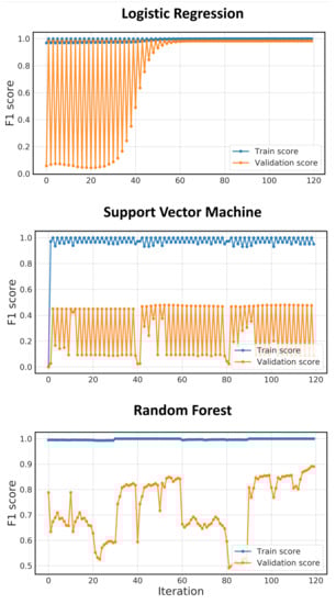
Figure A1.
Train and validation scores per gridsearch iteration for every model.
References
- Kates-Harbeck, J.; Svyatkovskiy, A.; Tang, W. Predicting disruptive instabilities in controlled fusion plasmas through deep learning. Nature 2019, 568, 526–531. [Google Scholar] [CrossRef] [PubMed]
- Samuell, C.M.; Mclean, A.G.; Johnson, C.A.; Glass, F.; Jaervinen, A.E. Measuring the Electron Temperature and Identifying Plasma Detachment Using Machine Learning and Spectroscopy. Rev. Sci. Instrum. 2021, 92, 043520. [Google Scholar] [CrossRef] [PubMed]
- Rea, C.; Montes, K.J.; Erickson, K.G.; Granetz, R.S.; Tinguely, R.A. A real-time machine learning-based disruption predictor in DIII-D. Nuclear Fusion 2019, 59, 096016. [Google Scholar] [CrossRef]
- Pavone, A.; Svensson, J.; Langenberg, A.; Höfel, U.; Kwak, S.; Pablant, N.; Wolf, R.C. Neural network approximation of Bayesian models for the inference of ion and electron temperature profiles at W7-X. Plasma Phys. Control. Fusion 2019, 61, 075012. [Google Scholar] [CrossRef]
- Kocsis, G.; Baross, T.; Biedermann, C.; Bodnar, G.; Cseh, G.; Ilkei, T.; König, R.; Otte, M.; Szabolics, T.; Szepesi, T.; et al. Overview video diagnostics for the W7-X stellarator. Fusion Eng. Des. 2015, 96–97, 808–811. [Google Scholar] [CrossRef]
- Zoletnik, S.; Biedermann, C.; Cseh, G.; Kocsis, G.; König, R.; Szabolics, T.; Szepesi, T. First results of the multi-purpose real-time processing video camera system on the Wendelstein 7-X stellarator and implications for future devices. Rev. Sci. Instrum. 2018, 89, 013502. [Google Scholar] [CrossRef] [PubMed] [Green Version]
- Biedler, C.; Grieger, G.; Herrnegger, F.; Harmeyer, E.; Kisslinger, J.; Lotz, W.; Maassberg, H.; Merkel, P.; Nührenberg, J.; Rau, F.; et al. Physics and Engineering Design for Wendelstein VII-X. Fusion Technol. 1990, 17, 148–168. [Google Scholar] [CrossRef]
- Bosch, H.-S.; Wolf, R.C.; Andreeva, T.; Baldzuhn, J.; Birus, D.; Bluhm, T.; Bräuer, T.; Braune, H.; Bykov, V.; Cardella, A.; et al. Technical challenges in the construction of the steady-state stellarator Wendelstein 7-X. Nuclear Fusion 2013, 53, 126001. [Google Scholar] [CrossRef]
- Bosch, H.-S.; Brakel, R.; Gasparotto, M.; Grote, H.; Hartmann, D.A.; Herrmann, R.; Nagel, M.; Naujoks, D.; Otte, M.; Risse, K.; et al. Transition from Construction to Operation Phase of the Wendelstein 7-X Stellarator. IEEE Trans. Plasma Sci. 2014, 42, 432–438. [Google Scholar] [CrossRef] [Green Version]
- Klinger, T.; Baylard, C.; Beidler, C.D.; Boscary, J.; Bosch, H.S.; Dinklage, A.; Hartmann, D.; Helander, P.; Maßberg, H.; Peacock, A.; et al. Towards assembly completion and preparation of experimental campaigns of Wendelstein 7-X in the perspective of a path to a stellarator fusion power plant. Fusion Eng. Des. 2013, 88, 461–465. [Google Scholar] [CrossRef] [Green Version]
- Pedersen, T.S.; König, R.; Krychowiak, M.; Jakubowski, M.; Baldzuhn, J.; Bozhenkov, S.; Fuchert, G.; Langenberg, A.; Niemann, H.; Zhang, D.; et al. First results from divertor operation in Wendelstein 7-X. Plasma Phys. Control. Fusion 2019, 61, 014035. [Google Scholar] [CrossRef] [Green Version]
- Krashennikov, S.I.; Kukushkin, A.S.; Pshenov, A.A. Divertor plasma detachment. Phys. Plasma 2016, 23, 055602. [Google Scholar] [CrossRef]
- Klinger, T.; Alonso, A.; Bozhenkov, S.; Burhenn, R.; Dinklage, A.; Fuchert, G.; Geiger, J.; Grulke, O.; Langenberg, A.; Hirsch, M.; et al. Performance and properties of the first plasmas of Wendelstein 7-X. Plasma Phys. Control. Fusion 2017, 59, 014018. [Google Scholar] [CrossRef]
- Klinger, T.; Andreeva, T.; Bozhenkov, S.; Brandt, C.; Burhenn, R.; Buttenschön, B.; Fuchert, G.; Geiger, B.; Grulke, O.; Laqua, H.P.; et al. Overview of first Wendelstein 7-X high performance operation. Nuclear Fusion 2019, 59, 112004. [Google Scholar] [CrossRef]
- Jakubowski, M.; Endler, M.; Feng, Y.; Gao, Y.; Killer, C.; König, R.; Krychowiak, M.; Perseo, V.; Reimold, F.; Schmitz, O.; et al. Overview of the results from divertor experiments with attached and detached plasmas at Wendelstein 7-X and their implications for steadystate operation. Nuclear Fusion 2021, 61, 106003. [Google Scholar] [CrossRef]
- Pedregosa, F. Scikit-learn: Machine Learning in Python. J. Mach. Learn. Res. 2011, 12, 2825–2830. [Google Scholar]
- James, G.M.; Witten, D.; Hastie, T.; Tibshirani, R. An Introduction to Statistical Learning, 2nd ed.; Springer: New York, NY, USA, 2021. [Google Scholar]
- scikit-learn.org. Available online: https://scikit-learn.org/stable/modules/generated/sklearn.linear_model.LogisticRegression.html (accessed on 20 December 2021).
- Feng, Y.; Jakubowski, M.; König, R.; Krychowiak, M.; Otte, M.; Reimold, F.; Reiter, D.; Schmitz, O.; Zhang, D.; Beidler, C.D.; et al. Understanding detachment of the W7-X island divertor. Nuclear Fusion 2021, 61, 086012. [Google Scholar] [CrossRef]
- Andreeva, T.; Kisslinger, J.; Wobig, H. Characteristics of main configurations of Wendelstein 7-X. Probl. At. Sci. Technol. Ser. Plasma Phys. 2002, 4, 45–47. [Google Scholar]
- Pedersen, T.S.; Szepesi, T.; Koenig, R.; Reimold, F.; Zhang, D.; Krychowiak, M.; Dinklage, A.; Kornejew, P.; Winters, V.; Hergenhahn, U.; et al. Small, stable plasmas, fully decoupled from the PFCs in W7-X. In Proceedings of the 62nd Annual Meeting of the APS Division of Plasma Physics, Online, 9–13 November 2020. [Google Scholar]
Publisher’s Note: MDPI stays neutral with regard to jurisdictional claims in published maps and institutional affiliations. |
© 2021 by the authors. Licensee MDPI, Basel, Switzerland. This article is an open access article distributed under the terms and conditions of the Creative Commons Attribution (CC BY) license (https://creativecommons.org/licenses/by/4.0/).