Battery Sizing for Mild P2 HEVs Considering the Battery Pack Thermal Limitations

Abstract

Small capacity and passively cooled battery packs are widely used in mild hybrid electric vehicles (MHEV). In this regard, continuous usage of electric traction could cause thermal runaway of the battery, reducing its life and increasing the risk of fire incidence. Hence, thermal limitations on the battery could be implemented in a supervisory controller to avoid such risks. A vast literature on the topic shows that the problem of battery thermal runaway is solved by applying active cooling or by implementing penalty factors on electric energy utilization for large capacity battery packs. However, they do not address the problem in the case of passive cooled, small capacity battery packs. In this paper, an experimentally validated electro-thermal model of the battery pack is integrated with the hybrid electric vehicle simulator. A supervisory controller using the equivalent consumption minimization strategy with, and without, consideration of thermal limitations are discussed. The results of a simulation of an MHEV with a 0.9 kWh battery pack showed that the thermal limitations of the battery pack caused a 2–3% fuel consumption increase compared to the case without such limitations; however, the limitations led to battery temperatures as high as 180 °C. The same simulation showed that the adoption of a 1.8 kWh battery pack led to a fuel consumption reduction of 8–13% without thermal implications.

1. Introduction

Powertrain hybridization seems to be a viable mid-term solution for the reduction of vehicle fuel consumption and tailpipe emissions [1,2,3,4]. Hybrid Electric Vehicles (HEVs) can be of series, parallel or combined (series-parallel, power-split) configurations [1,2]. Parallel configurations offer a cost-effective solution due to: easier integration of the HEV modules in an existing powertrain; the presence of a single electric motor (EM); and a small electric battery (especially in mild HEVs) [2,3].

Among parallel HEV architectures, the so-called P2 configuration is gaining the utmost attention of vehicle manufacturers as well as researchers due to its scalability and an increased number of operating modes [2,3,4]. As shown in Figure 1, in a P2 configuration, the electric machine (EM) is installed on the input shaft of the gearbox after the main clutch C0. Opening the C0 allows for driving in pure electric as well as for an efficient regeneration of the braking energy. By adding the clutch C1, the EM can be used as a starter to crank the ICE as well as for gear shifting.

Depending on the location of the EM, the P2 configuration can be on-axis or off-axis. The off-axis P2 HEVs have a stage of parallel axis gear, chain or belt drives (Figure 1) with advantages in terms of the axial size of the powertrain and the potential to have a smaller electric machine running at higher speed than the ICE.

Owing to the possibility of scaling the EM and the battery module, P2 is compatible with both mild and plug-in HEV, the mild P2 being characterized by a relatively smaller EM power and battery capacity [5,6]. An analysis of commercially available MHEVs shows that mostly they have a battery capacity in the range of 0.5–2 kWh [6,7].

Fuel consumption reduction is the main design goal of Mild HEVs, and this requires an integrated design of the powertrain components as well as the control strategy to avoid jeopardizing the vehicle’s dynamic performance [8,9]. A wide range of controllers has been proposed to this end in the literature. Rule-based supervisory controllers are the simplest to implement, however, they have limited performance when compared to optimization-based counterparts [10]. Optimization-based controllers like dynamic programming (DP) [9,10,11], equivalent consumption minimization strategy (ECMS) [11,12,13], and model predictive control (MPC) [14] are more performant in finding a global minimum of fuel consumption. However, they need a higher computational effort, require prior knowledge about the driving cycle, and hence can mainly be used in offline control strategies [10,13]. Comparable results to the ECMS can be obtained by implementing fuzzy logic rules, which can be very complex in the case of a large number of control variables [15].

The ECMS was first proposed by [12] as a real-time controller offering a near-optimal solution without prior knowledge of the drive cycle [13,16]. Furthermore, it allows for the constraint of various system variables by integrating them in a cost function by means of penalty functions. The main principle of the ECMS is to minimize the total equivalent fuel consumption at each time instant, including the contribution coming from the electrical energy to or from the battery. The optimization is constrained by the battery state of charge (SOC) and the maximum/minimum torque of the EM and ICE [12,15]. Additionally, it is well known that the battery is a safety-critical system that might cause a fire at high temperatures. Hence, most battery management systems (BMS) monitor the battery temperature in real-time to operate at less than 55 °C [16,17,18]. A review of fire incidence associated with electric and HEVs can be found in [19].

The control of the battery temperature can be accomplished by systems of different complexity, from simple passive cooling (heat is conducted through the battery casing and natural convection), to active cooling [17,18] (resorting to air or liquid as a coolant, or by other means such as using phase change materials [20]).

The influence of battery temperature on the performance and fuel consumption of HEV is discussed in [13], considering a 100 Ah capacity Lithium battery. Penalty factors for different ambient temperature and drive cycle combinations are integrated with the cost function of the ECMS supervisor. A battery aging semi-empirical model is taken into account along with its temperature dynamics, showing that cold ambient temperature causes a frequent charge and discharge of the battery due to the battery capacity reduction in cold ambient temperatures. The limitation of the electric traction due to high battery temperatures is not considered in the work [13].

Padovani et al. has studied how battery aging is affected by high or low temperatures, and high SOC [21]. A penalty for using the battery at high temperatures is included in the cost function. Considering a 7 kWh lithium-ion battery, an ambient temperature of 15 °C running on an Artemis drive cycle, the battery temperature does not exceed 35 °C. The lower operating temperatures in this work can be attributed to the large battery size.

Sarvaiya et al. [22] compared different control strategies incorporating the battery ageing model in the cost function. Considering the EPA driving cycle, and a pure electric vehicle with a relatively large 9 kWh lithium-ion battery, high temperatures are not an issue, with the temperature reaching 32 °C from a 30 °C ambient temperature.

An accurate electro-thermal model of the battery pack is needed to study the influence of the battery temperature in HEV. Battery heat generation induced by the electrical current can be divided into irreversible and reversible components [23,24]. The former is related to the Joule and polarization effects due to the current flowing through the internal resistance and charge transfer. The latter is due to the entropy change, which is related to the temperature dependence of the open circuit voltage (OCV). Barcellona and Piegari in [25] propose a model that can predict the thermal behaviour of a pouch lithium-ion battery cell based on its current and ambient conditions. The model only takes the effect of the OCV and internal resistance into account. However, the resistive-capacitive (RC) parallel branches are not included in the model of the battery, as the thermal time constant greatly outweighs the electrical one. Madani et al. in [26] review the determination of thermal parameters of a single cell, such as internal resistance, specific heat capacity, entropic heat coefficient, and thermal conductivity. These parameters are then used for the design of a suitable thermal management system. A lumped-parameter thermal model of a cylindrical LiFePO4/graphite lithium-ion battery is developed in [27] to compute the internal temperature.

Thermal management systems with active heating and cooling can be adopted for controlling the temperature in the battery pack [28,29,30]; however, the additional cost and complexity would not be affordable, especially in 48 V micro or mild hybrid electric vehicles. Conversely, 48 V micro or mild hybrids are potentially characterized by high-temperature fluctuations due to the large C-rate reached in boost and recuperation due to the small battery capacity.

The influence of battery temperature limitations on the fuel consumption of mild HEVs and the study of battery capacity, above which temperature does not represent a criticality, seems to be still largely unattended in the vast literature on the topic. Additionally, most of the literature that addresses energy management problems has adopted a simplified analytical model to estimate battery SOC and temperature. Such models can only be accurate under limited scenarios and hence could impose a limitation on model accuracy in a wider range of applications.

Hence, the main contribution of the present work is to address the following points: (a) to extend the existing control strategies to include the thermal limitations in the case of a 48 V P2 Mild HEV with passive cooling; (b) to validate the electro-thermal model of the battery by means of existing experimental data; and (c) to investigate the influence of the battery capacity on reaching thermal limitations and determine the minimum battery capacity to avoid thermal runaway.

The paper is organized as follows: In Section 2, the backward model of the conventional vehicle and P2 HEV are developed. The model of the conventional vehicle is validated using the experimental results reported in [31,32]. Furthermore, the electro-thermal model of the battery and its experimental validation are presented in this section. Section 3 presents the supervisory controller based on ECMS considering the thermal limitations of the battery. Section 4 reports the results of the simulation. Finally, Section 5 summarizes the main findings of the paper.

2. Vehicle Performance Modelling

The vehicle model shown in Figure 2 follows the backward approach widely adopted in the literature, especially for the design of the supervisory controller and the HEV components [11,33,34]. The detailed description of each subsystem and the underlying equations are given in the following table with reference to the HEV data summarized in

Table 1. Mazda CX9 2016 [31].

Parameter	Unit	Variable	Value
Vehicle
Nominal mass	kg	M	2041
Frontal Area	m2	Af	2.4207
Aerodynamic drag coefficient	-	Cx	0.316
Gear ratios	-	igb	1st—3.49; 2nd—1.99; 3rd—1.45; 4th—1; 5th—0.71; 6th—0.6
Final Drive Ratio	-	ifinal	4.41
Tire size	-		P255/50VR20
Passenger Capacity			7
Internal Combustion Engine
SAE Net Torque @ rpm	Nm		310 @ 2000
Fuel System	-		Gasoline Direct Injection
SAE Net power @ rpm	kW		169 @ 5000
Displacement	L		2.5
Electric Motor
Maximum power	kW		27
Maximum torque @ rpm	Nm	$T_{em.max}$	65 @ 4000
Battery (Sanyo NCR18650GA Lithium-ion cell)
Nominal voltage	V		3.6
Nominal capacity	Ah	$C_{tot}$	3.0
Minimum battery SOC	%	SOClow	60
Maximum battery SOC	%	SOChigh	80
Operating temperature	°C		−20~60
Ambient temperature	°C	${\theta }_{amb}$	20
Battery Pack Configurations	-		14s6p and 14s12p

.

2.1. Longitudinal Vehicle Dynamics

In this subsystem, the required traction force to overcome the resisting forces (i.e., aerodynamic and rolling resistance forces) is calculated as:

$$F_w=M\cdot dv/dt+M\cdot g\cdot f_r+\frac{1}{2}\cdot {\rho }_{air}\cdot C_x\cdot A_f\cdot v^2$$

(1)

where M is the vehicle mass; $v$ and $dv/dt$ are longitudinal speed and acceleration; $f_r$ is coefficient of rolling resistance; C_x is aerodynamic drag coefficient; ${\rho }_{air}$ is air density; $A_f$ is vehicle frontal area; F_W is the longitudinal force on the wheels. The resisting force due to road inclination is not considered in the analysis.

The total torque required on the wheels T_W, includes the drag torque in the axle bearings T_loss and torque due to inertia of the wheels J_W, they are added to the torque of the traction force on wheels F_W:

$$T_w=F_w\cdot R_w+4\cdot J_w\cdot \frac{dv}{dt}\cdot \frac{1}{R_w}+T_{loss}.$$

(2)

The wheel rolling radius R_W of the tire is calculated as:

$$R_w=\epsilon \cdot \left(\frac{D_{rim}\cdot 25.4}{2}+W\cdot \frac{AR}{100}\right).$$

(3)

The coefficient $\epsilon$ takes into account the tire deflection, which for radial tires is in the range $\epsilon =0.92-0.98$ [35]. The nominal wheel radius can be obtained from the tire markings, i.e., the rim diameter $D_{rim}$, nominal width $W$ and aspect ratio $AR$.

Moreover, the angular speed of the wheel shaft is then found from the rolling radius and the speed $v$:

$${\omega }_w=\frac{v}{R_w}.$$

(4)

2.2. Gearbox and Gearshift Logic

The gearbox model converts the wheel torque and speed to the corresponding ones at the input of the gearbox. A simple vehicle speed-based gearshift strategy is implemented in the model, accounting for the constraint of ICE maximum speed. Gearshift speeds are defined by analyzing the gearshift experimental data from Argon National Laboratory (ANL) Figure 3 shows the gearshift logic. To avoid frequent gear shifting, upshifts and downshifts are performed with a hysteresis that varies with the engaged gear.

The required torque $T_{gb}$ and angular speed ${\omega }_{gb}$ at the gearbox input can be computed from the final gear ratio $i_f$ and the gear ratio of the gearbox $i_{gb}$, as:

$$\{\begin{array}{c}{T}_{gb}=\frac{T_{axle}}{i_f\cdot {\eta }_f\cdot i_{gb}\cdot {\eta }_{gb}} if T_{axle}>0 \\ T_{gb}=\frac{T_{axle}\cdot {\eta }_f\cdot {\eta }_{gb}}{i_f\cdot i_{gb}} if T_{axle}\le 0\end{array}$$

(5)

where the efficiencies of the final gear and the gearbox are considered as ${\eta }_f={\eta }_{gb}=0.98$.

$${\omega }_{gb}={\omega }_w\cdot i_f\cdot i_{gb}$$

(6)

In a conventional vehicle $T_{gb}$ and ${\omega }_{gb}$ are the ICE torque and speed at the gearbox. When considering a HEV, the supervisory controller splits the same torque between the ICE and the EM depending on the established rules.

2.3. Internal Combustion Engine

The fuel consumption map of Mazda CX9 2016 ICE used in the simulation is shown in Figure 4 as obtained from experimental data [32]. The adoption of a static map typically leads to an estimate of the fuel consumption that is usually lower than what is measured in dynamic conditions by means of a chassis dynamometer [36]. However, this difference is in the range of 1–4% depending on the driving cycle [36], with more aggressive driving cycles being associated with the upper bound of this range. In this paper, the extra fuel consumption due to transient operation is neglected.

2.4. Electric Motor

For a given angular speed ${\omega }_{em}$ and a mechanical torque request $T_{em}$, the EM subsystem evaluates the electric power absorbed from the battery in discharge phases $P_{bat.dchg}$ or released to it during the charging phases $P_{bat.chg}$. This electric power is computed by means of the static efficiency map of the EM (Figure 5):

-

in discharging mode:

$$P_{bat.dchg}=\frac{P_{em}}{{\eta }_{em}}$$

(7)

-

in charging mode:

$$P_{bat.chg}=P_{em}\cdot {\eta }_{gen}$$

(8)

where the mechanical power $P_{em}$ is calculated as

$$P_{em}=T_{em}\cdot {\omega }_{em}$$

(9)

2.5. Battery Performance and Electro-Thermal Model

The essence of incorporating a battery electro-thermal model in the vehicle model (Figure 2) is to provide information to the ECMS controller for efficient fuel consumption minimization while preventing thermal runaway. At each time instant $k$, the adopted ECMS controller requires information of the state of charge $SOC\left(k\right)$, the temperature $\theta$, and the rate of the change of the temperature $\dot{\theta }$. This information is the output of the battery pack electro-thermal model that takes the power request $P_{bat}$ as input (from Equations (8) and (9). Considering the 14s6p battery configuration, the battery consists of a series module pack (SMP) composed of a series of fourteen (14) modules. Each of the modules consists of six (6) parallel cells, otherwise known as parallel cell modules (PCM).

The pack model is developed from the electro-thermal model of a single cell according to the work of [37]. First, an enhanced self-correcting (ESC) single-cell model is developed to form the building block for the PCM that is scaled to obtain the SMP. The resulting model is validated with an experimental dataset at an ambient environmental temperature of 20 °C.

The cell model takes into consideration both the static and the dynamic voltage characteristics as shown in Figure 6. A detailed description of each subsystem of the battery pack model is given below.

The static voltage computed from the OCV block is integrated with the dynamic voltage from the dynamic process to obtain an ESC cell model.

2.5.1. Static Component

The static component of the model represents the open-circuit voltage, which is the measured cell voltage when the cell is subject to a zero-load condition. The OCV is approximated as a function of only SOC for the temperature operating condition considered in this work. For the cell under consideration, the OCV is obtained from the cell datasheet of Sanyo NCR 18650-618 lithium-ion cell [38] that has a rated capacity of 3200 mAh. Figure 7 shows the voltage variation across SOC under open and closed-circuit conditions.

The middle blue curve shows the OCV as a function of SOC, as acquired from the datasheet. The red curve is the closed-circuit voltage at a constant charge load of 1.675 A. The yellow curve is the closed-circuit voltage at a constant discharge load of 0.66 A. It can be seen that the OCV taken from the datasheet approximates the true OCV at the mean of the closed-circuit voltages of the charge and discharge phases. The larger deviation of the charge phase results from the relative higher load with respect to the discharge phase.

The SOC is computed through coulomb counting and it is analogous to a fuel gauge that expresses the amount of charge contained in a cell. The expression of SOC is shown in Equation (10) for a given time step $k$.

$$SOC\left(k+1\right)=SOC\left(k\right)-\frac{\eta i\left(k\right)k}{C_{tot}}$$

(10)

where $i\left(k\right)$ is current input to the model—positive at discharge, $C_{tot}\left(\mathrm{Ah}\right)$ is the total releasable capacity in a complete cycle and $\eta$ is the battery coulombic efficiency. $SOC\left(k\right)$ is the SOC at kth time step. Only a percentage of current that is applied to the cell contributes to increasing the SOC in the charging phase. Hence, SOC is penalized with $\eta$ [30] in the charge phase.

2.5.2. Dynamic Component

The dynamic component of the cell model accounts for the voltage losses, including joule loss, diffusion loss due to mass transfer, activation loss due to charge transfer and loss due to hysteresis. The output of the dynamic model is the predicted closed-circuit voltage that accounts for these losses. The model is developed from an RC circuit with a single RC branch in series with a resistive branch [37] as shown in Figure 8.

The hyst component in the circuit accounts for the hysteretic contribution of the losses. The estimated dynamic voltage $\check{v}$ is computed as.

$$\check{v}\left(k\right)=OCV\left(SOC\left(k\right)\right) +v_{loss}\left(k\right)$$

(11)

$$v_{loss}\left(k\right)=Mh\left(k\right)+M_{0}s\left(k\right)-{{\displaystyle \sum }}_j{R}_j{i}_{Rj} \left(k\right)-R_{0}i\left(k\right)$$

(12)

where $v_{loss}$ is the voltage loss, $M_0$ is the instantaneous hysteresis voltage; $M$ is the dynamic hysteresis magnitude; $R_0$ is the instantaneous series resistor; $i_{Rj}\left(k\right)$ is the resistor diffusion current; $R_j$ is the parallel branch resistance; $h\left(k\right)$ is the hysteresis voltage; $s\left(k\right)$ is sign of current input. It is 1 for positive current input, −1 for negative input and zero otherwise.

The first two components at the right-hand side of Equation (12) model the instantaneous and the dynamic hysteresis voltage. The third component models the RC branch of the circuit. The subscript j represents the number of branches. The RC branch models the losses due to mass transport and charge transfer. The diffusion-resistor current $i_{Rj}$ that passes through the RC branch is computed from the time constant of the RC branch. The fourth component is the series resistive loss that models the joule losses.

The parameters of the model appear linearly according to Equation (13). $v_{loss}$ is computed for the $N$ data points of the experimental data and the parameters, $M, M_0, R_j, R_0$ are computed by least square approximation.

$$\left[\begin{array}{c}\begin{array}{c}{v}_{loss}\left(1\right)\\ v_{loss}\left(2\right)\\ ⋮\end{array}\\ v_{loss}\left(N\right)\end{array}\right]=\left[\begin{array}{c}\begin{array}{c}\begin{array}{ccc}h\left(1\right)& s\left(1\right)& -i_{R_j}^T\left(1\right)\end{array} -i\left(1\right)\\ \begin{array}{ccc}h\left(2\right)& s\left(2\right)& -i_{R_j}^T\left(2\right)\end{array} -i\left(2\right)\\ ⋮\end{array}\\ \begin{array}{ccc}h\left(N\right)& s\left(N\right)& -i_{R_j}^T\left(N\right)\end{array} -i\left(N\right)\end{array}\right] \left[\begin{array}{c}\begin{array}{c}M\\ M_0\\ R_j\end{array}\\ R_0\end{array}\right]$$

(13)

By least square approximation, $X=A \backslash Y$.

Table 2. List of electrical and thermal model parameters with the estimated values.

	Variable	Units	Value
Electric Model	Dynamic hysteresis magnitude, M	-	0.017
	$\mathrm{Instantaneous} \mathrm{hysteresis} \mathrm{height}, M_0$	-	negligible
	$\mathrm{Instantaneous} \mathrm{series} \mathrm{resistor}, R_0$	Ohms	0.024
	$\mathrm{Parallel} \mathrm{branch} \mathrm{resistance}, R_j$	Ohm	0.018
Thermal Model	$\mathrm{Specific} \mathrm{heat} \mathrm{capacity}, c_p$	$\mathrm{J}/\mathrm{kg}. \mathrm{K}$	1200
	$\mathrm{Thermal} \mathrm{resistance}, R_{conv}$	$\mathrm{K}/\mathrm{W}$	14.6
	$\mathrm{Cell} \mathrm{mass}, m_{cell}$	kg	48.5 × 10−3

reports the corresponding values of the electric and the thermal model parameters.

The dynamic current profile used for data collection during the experiment is applied as input to the model to compute $v_{loss}$ according to Equation (12). This profile consists of a sequence of random charge and discharge current values applied in the range of −4.5 A and +4.5 A. The current profile and $v_{loss}$ are shown in Figure 9.

2.5.3. The Battery Thermal Model

The thermal model is developed from contributions of the voltage losses that are computed from the dynamic voltage model of Equation (12). Based on lumped parameter assumption [39], the thermal model is designed based on heat transfer by convection and by neglecting the conduction heat transfer component according to Equation (14). The discrete-time battery surface temperature ${\theta }_{surf}$ is computed considering the power losses, $P_{loss}$ that is derived from the voltage losses, as the heat source.

$${\theta }_{surf}\left(k+1\right)={\theta }_{surf}\left(k\right)+\frac{T_s}{c_p\cdot m_{cell}}\left(P_{loss}\left(k\right)-\frac{{\theta }_{surf}\left(k\right)-{\theta }_{amb}}{R_{conv}}\right)$$

(14)

$c_p$ is the battery specific heat capacity; $m_{cell}$ is the cell mass; $P_{loss}$ is the power is computed based on the voltage losses; ${\theta }_{amb}$ is the ambient temperature; $T_s$ is the sampling time; $R_{conv}$ is the thermal resistance by convection. The thermal parameters are reported in Table 2.

3. Development of Supervisory Control Strategy

The supervisory control strategy based on the Equivalent Consumption Minimization Strategy optimally splits the required traction torque $T_{gb}$ between the traction sources while minimizing the objective function. In this section, three types of ECMS are demonstrated. The first type is the ECMS without considering the battery thermal limitations. The second type is an ECMS with an on/off switching of the electric traction when the battery temperature threshold is reached. Finally, in the third type, the thermal limitations are integrated into the penalty functions on the temperature and the temperature dynamics are set in the objective function.

3.1. ECMS Control Strategy without Thermal Limitations

To achieve an effective reduction in fuel usage, the contribution of electric motor power should be defined in such a way that the engine operates in its higher efficiency zone. For this reason, the ECMS was applied to the MHEV backward model to determine the power split ratio between the engine and the EM. From the configuration of the MHEV system, the rotational speeds of the power sources are set by vehicle velocity. Hence, the ECMS controller splits only the torque between the engine and EM.

Objective function:

The objective function for the ECMS is overall equivalent fuel consumption ($J_{ecms}$) which is evaluated as a sum of engine fuel consumption ${\dot{m}}_{ice}$ and equivalent fuel consumption of the electric power usage ${\dot{m}}_{eqv}$ for the power drawn from the battery $P_{bat}$ [10,12]:

$$J_{ecms}={\dot{m}}_{ice}\left(P_{ice}\right)+{\dot{m}}_{eqv}\left(P_{bat}\right)$$

(15)

${\dot{m}}_{eqv}\left(P_{bat}\right)$equivalent fuel consumption of EM can be computed as the fuel consumption of the ICE to provide the same mechanical power generated by electric motor [12]:

$${\dot{m}}_{eqv}\left(P_{bat}\right)=P_{em}\left(T_{em},{\omega }_{em}\right)\cdot s_{eqv}=T_{em}\cdot {\omega }_{em}\cdot s_{eqv}$$

(16)

$s_{eqv}$ is the battery equivalent fuel consumption factor, depending on battery discharging ($P_{bat}>0$) or charging ($P_{bat}<0$) modes as:

$$s_{eqv}=\{\begin{array}{l}\frac{1}{LHV\cdot {\eta }_{ice}\cdot {\eta }_{em}\cdot {\eta }_{inv}\cdot {\eta }_{bat} } \left(P_{bat}>0\right)\\ 0 \left(P_{bat}=0\right)\\ \frac{1}{LHV\cdot {\eta }_{ice}}\cdot {\eta }_{em}\cdot {\eta }_{inv}\cdot {\eta }_{bat} \left(P_{bat}<0\right)\end{array}$$

(17)

where $LHV$ is the lower heating value of the fuel, ${\eta }_{ice}$ is the average efficiency of the ICE, ${\eta }_{em}$ is the average efficiency of the EM and ${\eta }_{inv}$ is the average efficiency of the inverter.

The mathematical model for ICE fuel consumption rate ${\dot{m}}_{ice}$ at a given operation point $\left(T_{ice}, {\omega }_{ice}\right)$ was obtained by steady state curve fitting of the engine map data (see Figure 10). The regression coefficients of the polynomial function (see Equation (18)) were estimated accurately since the goodness of this fitting indicated R-square = 0.9961.

$$\begin{gathered} {\dot{m}}_{ice}\left(T_{ice}, {\omega }_{ice}\right)=p_{00}+p_{10}\cdot {\omega }_{ice}+p_{01}\cdot T_{ice}+p_{20}\cdot {\omega }_{ice}^2+\dots \\ +p_{11}\cdot {\omega }_{ice}\cdot T_{ice}+p_{02}\cdot T_{ice}^2+p_{21}\cdot {\omega }_e^2\cdot T_{ice}+\dots \\ +p_{12}\cdot {\omega }_e\cdot T_{ice}^2+p_{03}\cdot T_{ice}^3 \end{gathered}$$

(18)

Once the objective function is expressed as a function of EM torque and engine torque (independent variables), then constraints were constituted based on operation limits and satisfying the required torque demand of the vehicle.

Constraints:

As shown in Equation (19), a necessary condition is to provide the required torque and request that the sum of torque contributions of two sources at the output of the gearbox be equal to torque demand at the same level. Moreover, the ICE and EM torques must be within the corresponding operating envelope:

$$\{\begin{array}{c}{T}_{gb}=(T_{em}\cdot U_{pulley}+T_{ice})/i_{gb}\\ 0\le T_{ice}\le T_{ice.max}\\ -T_{em.max}\le T_{em}\le T_{em.max}\end{array}$$

(19)

where, $U_{pulley}$—gear ratio on the pulley that connects EM to the input shaft of the gearbox and $i_{gb}$—gear ratio of engaged gears in the gearbox.

By minimizing the objective function (Equation (15)) over the range described in the constraints (Equation (18)), the optimum value of $(T_{ice}, T_{em}$) can be estimated instantly, without considering the SOC level. When SOC is too low, the controller must restrict usage of the EM. On the other hand, when the SOC is near its upper threshold limit, the controller tends to use the EM power. Moreover, to accurately compare the fuel consumption of HEV, results should be indicated for the charge sustaining mode where SOC has the same level at the beginning and at the end of the driving cycle.

Charge sustaining mode:

Therefore, to maintain the battery SOC within the lower $SO{C}_{low}$ and upper $SO{C}_{high}$ limits, an s-shaped correction function $P{F}_{soc}$ was introduced to penalize the equivalent fuel consumption of the battery [10]. If the SOC decreases below the threshold (0.6 in this case), the vehicle tends to restrict the usage of electric energy, hence the $P{F}_{soc}$ starts to rise. Otherwise, the correction factor is equal to 1, meaning that no limitation to utilize the electric power is applied. In terms of an equation, the above condition can be represented as:

$$P{F}_{soc}=\{\begin{array}{cc}1-0.15 {\overline{SOC}}^3+0.05 {\overline{SOC}}^4,& SOC<0.6\\ 1,& SOC\ge 0.6\end{array}$$

(20)

where $\overline{SOC}$ is a normalized state of charge that can be computed as [10]:

$$\overline{SOC}=\frac{2\cdot SOC-\left(SO{C}_{high}+SO{C}_{low}\right)}{SO{C}_{high}-SO{C}_{low}}$$

(21)

where, $SO{C}_{high}=0.80$ and $SO{C}_{high}=0.60$ values are used as upper and lower threshold limits for SOC of the battery.

The coefficients in Equation (20) are chosen based on multiple trials to obtain the best fuel consumption.

The plot in Figure 11 shows the variation of $P{F}_{soc}$ as a function of SOC.

Then the objective function in Equation (15) is modified with the penalization for low SOC values, as:

$$J_{ecms}={\dot{m}}_{ice}\left(P_{ice}\right)+P{F}_{soc}\cdot {\dot{m}}_{eqv}\left(P_{bat}\right)$$

(22)

By minimizing this objective function, the torque split is performed to minimize the fuel consumption without considering the thermal limitations of the battery. However, as was mentioned, the optimal operating temperature range for lithium-ion batteries is between $15–55 °\mathrm{C}$, otherwise, their safety, power and life are impacted [17,18,20]. Therefore, temperature limitation will be implemented in the ECMS controller in the next step.

3.2. ECMS Control Strategy with Thermal Limitations Using Temperature Threshold

To avoid the thermal runaway of the battery, limitations can be applied by setting the battery temperature ${\theta }_{bat}$ threshold to 55 °C. Over this temperature, the usage of electric power is limited. Hence, the required power is provided mainly by the ICE. This is implemented by setting the penalty factor $P{F}_{SO}$ to a huge number when the battery temperature is over the given threshold as shown in Equation (23). As can be seen, if the battery temperature is ${\theta }_{bat}>55$ °C the penalty factor is set to a very high number i.e., to 1000, regardless of the battery SOC.

$$P{F}_{soc}^{\theta }=\{\begin{array}{ccc}\hfill 1-0.15 {\overline{SOC}}^3+0.05 {\overline{SOC}}^4,\hfill & \hfill if {\theta }_{bat}\le 55 °\mathrm{C}& and SOC<0.6\hfill \\ \hfill 1,\hfill & \hfill if {\theta }_{bat}\le 55 °\mathrm{C}& and SOC\ge 0.6\hfill \\ \hfill 1000,\hfill & \hfill {\theta }_{bat}>55 °\mathrm{C}& \end{array}$$

(23)

Then, the penalty factor $P{F}_{soc}$ in Equation (22) is replaced with the penalty factor $P{F}_{soc}^{\theta }$ which considers the thermal condition of the battery as well. By implementing such a limitation, the penalty factor works as an on/off switch triggered by the temperature threshold and battery operation outside of the designed operating temperature range can be avoided. However, this limitation does not include the rate of temperature change, which might result in a temperature overshoot due to a previous power drain from the battery. In the next step, the temperature change rate is also limited.

3.3. ECMS Control Strategy with Thermal Limitations Using Penalty Function on Temperature and Temperature Change Rate

To avoid thermal shocks in the battery, the penalty factor is represented as a cumulative product of penalty factors on the temperature $P{F}_{\theta }$, on the temperature change rate $P{F}_{\dot{\theta }}$ and on the SOC $P{F}_{soc}$ are applied to equivalent fuel consumption (${\dot{m}}_{eqv}$) of the electric motor:

$$J_{ecms}={\dot{m}}_{ice} \left(P_{ice}\right)+P{F}_{\theta }\cdot P{F}_{\dot{\theta }}\cdot P{F}_{soc}\cdot {\dot{m}}_{eqv}\left(P_{bat}\right)$$

(24)

The penalty function on temperature $P{F}_{\theta }$ is defined as:

$$P{F}_{\theta }=1+1.75\cdot {\overline{\theta }}^3$$

(25)

where $\overline{\theta }$ is normalized temperature calculated as a function of upper ${\theta }_{high}$ and lower ${\theta }_{low}$ temperature limit as [10]:

$$\overline{\theta }=\frac{2\cdot {\theta }_{bat}-\left({\theta }_{high}+{\theta }_{low}\right)}{{\theta }_{high}-{\theta }_{low}}$$

(26)

where: ${\theta }_{low}=10 °\mathrm{C}$ and ${\theta }_{high}=60 °\mathrm{C}$.

Function of $P{F}_{\theta }$ is plotted in Figure 12a, it has a value of about 1 when the battery temperature is lower than 40 °C. As the battery temperature increases beyond 40 °C, a correction factor $P{F}_{\theta }$ gets higher value, so usage of EM power will be limited.

The penalty on the temperature change rate $P{F}_{\dot{\theta }}$ is used to avoid a high-temperature change rate which could induce the thermal shock on the battery is:

$$P{F}_{\dot{\theta }}=1+1\cdot {\overline{\dot{\theta }}}^3$$

(27)

where $\overline{\dot{\theta }}$ is normalized temperature change rate, a function of upper ${\dot{\theta }}_{high}$ and lower ${\dot{\theta }}_{low}$ temperature change limits [10]:

$$\overline{\dot{\theta }}=\frac{2\cdot \dot{\theta }-\left({\dot{\theta }}_{high}+{\dot{\theta }}_{low}\right)}{{\dot{\theta }}_{high}-{\dot{\theta }}_{low}}$$

(28)

where for upper and lower limits for rate of temperature change are:

$${\dot{\theta }}_{low}=0 °\mathrm{C}/\mathrm{s} and {\dot{\theta }}_{high}=6 °\mathrm{C}/\mathrm{s}$$

The graphical representation of $P{F}_{\dot{\theta }}$ is given in Figure 12b.

4. Results and Experimental Validation of the Developed Model

An intermediate step of the HEV modelling was to validate the conventional vehicle model by comparing it to experimental data. To validate the model, experimental data from ANL [31] for a conventional vehicle was compared with the results of the developed model simulation. Furthermore, the battery electro-thermal model was validated experimentally using a developed test bench that was developed in-house. The simulation model of the mild P2 HEV is discussed afterwards in this section.

4.1. Experimental Validation of Conventional Vehicle Model

The conventional vehicle model was obtained by disabling the ECMS controller, Electric Machine, and Battery Electro-Thermal model subsystems. This vehicle model was designed based on a backward model was developed in Matlab/Simulink environment using all characteristics and parameters of the selected vehicle. The model estimates the fuel consumption of the vehicle by computing the required ICE speed (${\omega }_{ice}$) and torque ($T_{ice}$) for a given driving cycle. To validate the model, experimental test data of the powertrain components and of the vehicle from ANL were used. The data includes measurements of the vehicle speed ($v$), the ICE torque ($T_{ice}$) and its angular speed $({\omega }_{ice}$), the selected gear ($i_{gr}$), and the instantaneous fuel consumption (${\dot{m}}_{ice}$) profile. A Mazda CX9 2016 SUV was selected for further analysis. The complete data of the ICE map and the vehicle parameters are available in [32]. For the validation, the simulated value of the torque, the angular speed and the fuel consumption rate of the ICE, and the engaged gear of the gearbox were compared to those from the experiments reported by ANL.

As is shown in Figure 13, the input is the speed profile of the UDDS driving cycle. The gearshift in the model is defined on the basis of the vehicle velocity and the result of the gear ratio is almost overlapping with the ANL experimental data (Figure 13b). Moreover, the simulated values of the ICE angular speed (Figure 13c) and the torque (Figure 13d) reported at the output of the gearbox show a good match with experimental data. For the calculation of the tire radius (Equation (3)), the coefficient $\epsilon$ was chosen to be equal to 0.95. The simulated and experimental values for the fuel rate (Figure 13e) have slight differences, due to the fact that transient fuel consumption is not taken into account. Figure 13e visualizes this fact, where the differences are mainly in the transient phases, which was not modelled. For the total fuel consumed during the UDDS cycle, a simulated value of 699 g vs. an experimental value of 739 g was obtained. This corresponds to a difference of about 5%. However, if transient fuel consumption behaviour of the engine is excluded this difference is within just 2% (713 g), while the other 3% of the difference is due to transient phenomena which is not included in the developed model as mentioned above.

4.2. Electro-Thermal Model Validation

The Electro-thermal model was experimentally validated using the experimental test bench described in Figure 14. The test bench consisted of six cells connected in a series with voltage across the cells measured with Elithion cell boards. An LM35 Texas Instrument temperature sensor was used to measure the cell surface temperature. An Elithion (Lithiumate) Battery Management System (BMS) was installed on the test bench to enhance the safety of the acquisition process. An Arduino Mega board connected via LAN to a dedicated PC was then used to acquire the measured data. As an extra safety measure, the system was equipped with an emergency stop device.

The experimental data consisting of a dynamic current (A) input, battery surface temperature (°C) and voltage (V) outputs were collected at room temperature from an NRC18650G-HOANA cell of 3200 mAh rated capacity. The dynamic current input was in the range of $\pm 4.5 \mathrm{A}$ for both the charge and discharge phases. With the experiment conducted at ambient temperature, the estimated and the measured voltages were compared as in Figure 15b. The thermal model was equally validated, and the result is shown in Figure 15c.

4.3. Parallel Cell Module (PCM)

With the single-cell model designed and validated, the model forms a building block for developing the PCM and the SMP for further integration in a complete vehicle model.

A battery PCM consists of cells that are connected in parallel while the SMP consists of battery modules that are connected in series to make a battery pack. A 14s6p battery pack configuration entails 14 SMP and six PCM. The parallel cell configuration is often useful for increasing the energy capacity of the battery pack, especially for various high energy applications.

The current through each cell in a module $i_j$ can be computed from Equation (29) if the module voltage $v$ can be derived. By Kirchhoff’s law, the sum of all the individual current that passes through a module is equal to the pack current. Also, the voltages at the terminal of all the cells in the module are equal. The cell voltage has two contributions: the instantaneous voltage that changes instantly with the current and the non-instantaneous state voltages $v_f$.

$$v\left(k\right)=v_{f,j}\left(k\right)-i_j\left(k\right)R_{0,j}$$

(29)

$R_0$ of the joule, the loss is modified to accommodate the cell terminal losses.

The sum of the current through the individual cells in module $i$ can be computed from Equation (29).

$$i\left(k\right)={\displaystyle \sum }_j^p\left(\frac{v_{f,j}\left(k\right)-v\left(k\right) }{R_{0,j}}\right)$$

(30)

$p$ is the number of parallel branches in the module and $j$ is the branch index.

By simultaneous computation of Equations (29) and (30), the current through each cell in the module and the voltage can be derived. The modules are connected in series to develop an SMP. To design a 48 V, 0.9 kWh battery pack, a 14s6p configuration was used.

The temperature distribution within the battery pack was evaluated on the basis of the variation of the SOC and the capacity of the cells within the battery pack. The battery pack was simulated to show these variations. Figure 16a shows the variation of temperature when the initial SOC varies from 0.85 to 0.95, assuming an equal total capacity of 3.0 Ah for the individual cells. Figure 16b shows the variation of temperature when the cell capacity varies from 2.7 Ah to 3.0 Ah, assuming equal initial SOC of 0.95 for all cells.

Based on the result of the simulation shown in Figure 16, the maximum temperature of the battery pack is in the range of 60 °C to 70 °C at the end of the tests. The temperature variation is larger for varying SOC than for varying capacity.

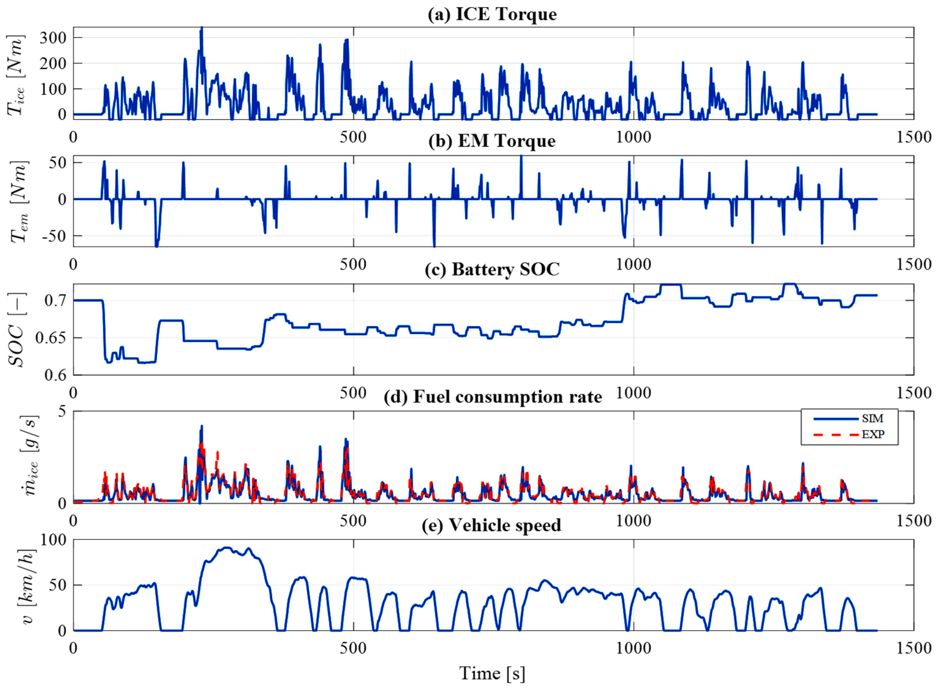
4.4. Simulation Results for P2 HEV

Once the simulation model was validated experimentally, the simulation was performed with the P2 HEV (with 14s6p battery pack) complete simulation model on different driving cycles (UDDS, NEDC and WLTC). As an example, the results for UDDS driving cycle with three levels of limitations are presented in Figure 17, Figure 18 and Figure 19. The figures represent (a) ICE torque, (b) EM torque, (c) the battery SOC, (d) fuel consumption rate and (e) the speed profile on UDDS driving cycle. Note that here, results are shown for when the C0 clutch was engaged during the declaration phase, which means that regenerative braking will be affected by the resistive torque of the engine. In all the cases, the SOC was maintained at the beginning and at the end of driving cycle. For this reason, the initial SOC was varied in different cases to ensure the electrical energy equilibrium. The overall fuel efficiency was improved by 8.6% compared to conventional vehicle simulation results (699.9 g) in the case where no thermal limitations are applied (Figure 17). However, the temperature of the battery reached about 160 °C (see Figure 19a solid blue line) under UDDS cycle.

In Figure 18, results are described for ECMS with thermal limitation implemented by means of an on/off penalty factor (discussed in Equation (22)). In this case, the overall fuel consumption was reduced by only 3.8% compared to the conventional vehicle model (699.9 gr). Since, traction power contribution by EM is possible only if battery temperature is below 55 °C (see Figure 19a).

With the penalty factors on both the temperature $P{F}_{\theta }$ and the temperature change rate $P{F}_{\dot{\theta }}$ (discussed in Equations (24)–(27)), the battery temperature was kept below 55 °C (see Figure 20a), and overall fuel usage was improved by 4.8% with respect to conventional vehicle model as in Figure 19.

The temperature profile of the battery for UDDS, NEDC and WLTC driving cycles are given in Figure 20. For the case with no thermal limitations (blue, solid lines), the more aggressive cycles such as UDDS and WLTC have higher power demand, therefore, the temperature of the battery went up to 160 °C and 180 °C (Figure 20a,c), respectively. The temperature for the low power demanding NEDC cycle stayed within 85 °C (Figure 20b).

The case with limitation on both temperature and temperature change rate (yellow, dotted line) showed more stable the battery temperature profile compared to the on/off temperature limitation (orange, dashed line) strategy. The reason is that introducing penalty factor due to the temperature changing rate $P{F}_{\dot{\theta }}$, which limits the rapid changes in the battery temperature. Moreover, in three driving cycles (UDDS, NEDC, and WLTC) this limitation led to fuel consumption improvement of 1%, 0.3% and 0.7%, respectively, compared to the on/off strategy.

As can be seen, the introduction of the thermal limitation positively affects the thermal behaviour that helps to avoid the thermal runaway. However, fuel economy is negatively affected, as the use of electric traction is limited as well.

Therefore, it would be reasonable to define the minimum capacity of the battery that allows avoiding thermal runaway without introducing the thermal limitation on the control strategy.

4.5. Increased Battery Size to Avoid Temperature Limits (14s12p)

To reduce the fuel consumption of the vehicle while keeping the thermal condition of the battery within the optimal range, the battery pack capacity was doubled. Since an increase of the number of parallel cells results in a decrease of the current per cell, this should affect positively the battery thermal behavior. Therefore, the number of parallel cells was gradually increased (using integer numbers only) from 14s6p to obtain a 14s12p configuration. The profile of the different variables over the WLTC cycle is shown in Figure 21.

The results show (Figure 22) that starting from a 14s12p configuration the battery temperature stays within the optimal range, even in the most aggressive cycle considered in the study. The results for this configuration are 50 °C, 37 °C and 61 °C in the UDDS, NEDC and WLTC cycles, respectively. The fuel consumption and its percentage reduction (in brackets) relative to the conventional vehicle are as follows: 611.4 g (−12.6%), 544 g (−8.2%) and 1185 g (−9.4%), for the UDDS, NEDC and WLTC driving cycles, respectively.

5. Discussion and Conclusions

Table 3. Main results of the simulation.

Drive Cycle	Fuel Consumption [g] Fuel Economy [%] Max Temperature [°C]
	Conventional Vehicle		14s6p: ECMS no Limitation			14s6p: ECMS with On/off			14s6p: ECMS with Penalty			14s12p: ECMS no Limitation
UDDS	699.9	100%	639.9	−8.6%	160 °C	673	−3.8%	55 °C	666.2	−4.8%	55 °C	611.4	−12.6%	50 °C
NEDC	592.3	100%	556	−6.1%	85 °C	563	−4.9%	55 °C	561.6	−5.2%	55 °C	544	−8.2%	37 °C
WLTC	1308	100%	1218	−6.9%	180 °C	1269	−2.9%	55 °C	1261	−3.6%	55 °C	1185	−9.4%	61 °C

summarizes the simulation results for P2 mild HEV with a 48 V 0.9 kWh (14s6p) battery pack. It includes the overall fuel consumption, the percentage of reduction with reference to conventional vehicles and the maximum temperature over the corresponding cycle. Furthermore, the results for the 14s12p battery pack with increased capacity (1.8 kWh) and without thermal limitations implemented in the supervisory controller are reported.

The considered battery packs have a passive cooling system. Hence the heat transfer is only by natural convection. Therefore, thermal limitations must be applied on the controller level for the 14s6p battery pack to limit battery usage and to avoid thermal runaway. However, the implementation of limitations on the controller leads to a fuel consumption increase of between 2–3%. To achieve a reduction in fuel consumption without compromising thermal behaviour, a larger battery capacity could be considered. The minimum battery capacity would be 1.8 kWh, which corresponds to a 14s12p battery pack configuration. Fuel consumption in this case is reduced by between 8–13% with reference to the fuel consumption of the conventional vehicle.

Obviously, the increase of ambient temperature should change the minimum battery capacity towards the higher values. However, the analysis was conducted considering a constant ambient temperature of 20 °C. The influence of different ambient temperatures has not been validated in this work and can be addressed in future works.

References

1. Ehsani, M.; Gao, Y.; Emadi, A. Modern Electric, Hybrid Electric, and Fuel Cell Vehicles; CRC Press: Boca Raton, FL, USA, 2017. [Google Scholar] [CrossRef]
2. Sieg, C.; Küçükay, F. Benchmarking of Dedicated Hybrid Transmissions. Vehicles 2020, 2, 6. [Google Scholar] [CrossRef] [Green Version]
3. Rahman, Z.; Butler, K.L.; Ehsani, M. A Comparison Study Between Two Parallel Hybrid Control Concepts. SAE Tech. Pap. Ser. 2000. [Google Scholar] [CrossRef]
4. Sundström, O.; Guzzella, L.; Soltic, P. Optimal Hybridization in Two Parallel Hybrid Electric Vehicles Using Dynamic Programming. IFAC Proc. Vol. 2008, 41, 4642–4647. [Google Scholar] [CrossRef] [Green Version]
5. Emadi, A. Advanced Electric Drive Vehicles; CRC Press: Boca Raton, FL, USA, 2014. [Google Scholar] [CrossRef]
6. Zhang, B.; Yang, F.; Teng, L.; Ouyang, M.; Guo, K.; Li, W.; Du, J. Comparative Analysis of Technical Route and Market Development for Light-Duty PHEV in China and the US. Energies 2019, 12, 3753. [Google Scholar] [CrossRef] [Green Version]
7. Ruzimov, S.; Mavlonov, J.; Mukhitdinov, A. Analysis of the Powertrain Component Size of Electrified Vehicles Commercially Available on the Market. Commun. Sci. Lett. Univ. Zilina 2022, 24, B74–B86. [Google Scholar] [CrossRef]
8. Hofman, T.; Ebbesen, S.; Guzzella, L. Topology Optimization for Hybrid Electric Vehicles with Automated Transmissions. IEEE Trans. Veh. Technol. 2012, 61, 2442–2451. [Google Scholar] [CrossRef] [Green Version]
9. Silvas, E.; Hofman, T.; Murgovski, N.; Etman, P.; Steinbuch, M. Review of Optimization Strategies for System-Level Design in Hybrid Electric Vehicles. IEEE Trans. Veh. Technol. 2016, 66, 57–70. [Google Scholar] [CrossRef]
10. Liu, X.; Qin, D.; Wang, S. Minimum Energy Management Strategy of Equivalent Fuel Consumption of Hybrid Electric Vehicle Based on Improved Global Optimization Equivalent Factor. Energies 2019, 12, 2076. [Google Scholar] [CrossRef] [Green Version]
11. Onori, S.; Serrao, L.; Rizzoni, G. Hybrid Electric Vehicles; Springer: London, UK, 2016. [Google Scholar] [CrossRef]
12. Paganelli, G.; Delprat, S.; Guerra, T.M.; Rimaux, J.; Santin, J.J. Equivalent Consumption Minimization Strategy for Parallel Hybrid Powertrains. Vehicular Technology Conference. In Proceedings of the IEEE 55th Vehicular Technology Conference; VTC Spring: 2002, (Cat. No.02CH37367), Birmingham, AL, USA, 6–9 May 2002. [Google Scholar] [CrossRef]
13. Zhou, B.; Rezaei, A.; Burl, J. Effect of Battery Temperature on Fuel Economy and Battery Aging When Using the Equivalent Consumption Minimization Strategy for Hybrid Electric Vehicles. In SAE Technical Paper Series; SAE International: Warrendale, MI, USA, 2020. [Google Scholar] [CrossRef]
14. Yu, K.; Tan, X.; Yang, H.; Liu, W.; Cui, L.; Liang, Q. Model Predictive Control of Hybrid Electric Vehicles for Improved Fuel Economy. Asian J. Control 2016, 18, 2122–2135. [Google Scholar] [CrossRef]
15. Rahmeh, H.; Bonfitto, A.; Ruzimov, S. Fuzzy Logic vs Equivalent Consumption Minimization Strategy for Energy Management in P2 Hybrid Electric Vehicles. In Volume 4: 22nd International Conference on Advanced Vehicle Technologies (AVT); USA American Society of Mechanical Engineers: St. Louis, MO, USA, 2020. [Google Scholar] [CrossRef]
16. Conte, F.V. Battery and Battery Management for Hybrid Electric Vehicles: A Review. Elektrotech. Inftech. 2006, 123, 424–431. [Google Scholar] [CrossRef]
17. MAHLE Powertrain High Charge Rate 48 V Battery Pack. Available online: https://www.mahle-powertrain.com/media/mahle-powertrain/experience/48v-battery-pack/mpt-48-v-battery.pdf (accessed on 20 June 2021).
18. Vehicle Energy Japan: Lithium-ion Battery Pack for 48 V HEV. Available online: https://www.ve-j.co.jp/en/product-03.html (accessed on 23 December 2021).
19. Sun, P.; Bisschop, R.; Niu, H.; Huang, X. A Review of Battery Fires in Electric Vehicles. Fire Technol. 2020, 56, 1361–1410. [Google Scholar] [CrossRef]
20. Javani, N.; Dincer, I.; Naterer, G.F.; Yilbas, B.S. Exergy Analysis and Optimization of a Thermal Management System with Phase Change Material for Hybrid Electric Vehicles. Appl. Therm. Eng. 2014, 64, 471–482. [Google Scholar] [CrossRef]
21. Padovani, T.M.; Debert, M.; Colin, G.; Chamaillard, Y. Optimal Energy Management Strategy including Battery Health through Thermal Management for Hybrid Vehicles. IFAC Proc. Vol. 2013, 46, 384–389. [Google Scholar] [CrossRef] [Green Version]
22. Sarvaiya, S.; Ganesh, S.; Xu, B. Comparative Analysis of Hybrid Vehicle Energy Management Strategies with Optimization of Fuel Economy and Battery Life. Energy 2021, 228, 120604. [Google Scholar] [CrossRef]
23. Schuster, E.; Ziebert, C.; Melcher, A.; Rohde, M.; Seifert, H.J. Thermal Behavior and Electrochemical Heat Generation in a Commercial 40 Ah Lithium Ion Pouch Cell. J. Power Sources 2015, 286, 580–589. [Google Scholar] [CrossRef]
24. Xiao, M.; Choe, S.-Y. Dynamic Modeling and Analysis of a Pouch Type LiMn2O4/Carbon High Power Li- Polymer Battery Based on Electrochemical-Thermal Principles. J. Power Sources 2012, 218, 357–367. [Google Scholar] [CrossRef]
25. Barcellona, S.; Piegari, L. Integrated Electro-Thermal Model for Pouch Lithium Ion Batteries. Math. Comput. Simul. 2021, 183, 5–19. [Google Scholar] [CrossRef]
26. Madani, S.; Schaltz, E.; Knudsen Kær, S. Review of Parameter Determination for Thermal Modeling of Lithium Ion Batteries. Batteries 2018, 4, 20. [Google Scholar] [CrossRef] [Green Version]
27. Forgez, C.; Vinh Do, D.; Friedrich, G.; Morcrette, M.; Delacourt, C. Thermal Modeling of a Cylindrical LiFePO4/Graphite Lithium-Ion Battery. J. Power Sources 2010, 195, 2961–2968. [Google Scholar] [CrossRef]
28. Worwood, D.; Kellner, Q.; Wojtala, M.; Widanage, W.D.; McGlen, R.; Greenwood, D.; Marco, J. A New Approach to the Internal Thermal Management of Cylindrical Battery Cells for Automotive Applications. J. Power Sources 2017, 346, 151–166. [Google Scholar] [CrossRef]
29. Zhao, C.; Sousa, A.C.M.; Jiang, F. Minimization of Thermal Non-Uniformity in Lithium-Ion Battery Pack Cooled by Channeled Liquid Flow. Int. J. Heat Mass Transf. 2019, 129, 660–670. [Google Scholar] [CrossRef]
30. Bai, F.; Chen, M.; Song, W.; Li, Y.; Feng, Z.; Li, Y. Thermal Management of 48 V Standby Battery for Outdoor Base Station at Cold Environment. Energy Procedia 2019, 158, 4224–4231. [Google Scholar] [CrossRef]
31. Available online: https://www.anl.gov/es/energy-systems-d3-2016-mazda-cx9 (accessed on 2 December 2021).
32. Available online: https://www.epa.gov/vehicle-and-fuel-emissions-testing/combining-data-complete-engine-alpha-maps (accessed on 2 December 2021).
33. Horrein, L.; Bouscayrol, A.; Delarue, P.; Verhille, J.N.; Mayet, C. Forward and Backward Simulations of a Power Propulsion System. IFAC Proc. Vol. 2012, 45, 441–446. [Google Scholar] [CrossRef] [Green Version]
34. Guzzella, L.; Sciarretta, A. Vehicle Propulsion Systems; Springer: Berlin/Heidelberg, Germany, 2013. [Google Scholar] [CrossRef]
35. Genta, G. Motor Vehicle Dynamics: Modeling and Simulation; Series on Advances in Mathematics for Applied Sciences; World Scientific: Singapore, 1997. [Google Scholar] [CrossRef]
36. Dekraker, P.; Stuhldreher, M.; Kim, Y. Characterizing Factors Influencing SI Engine Transient Fuel Consumption for Vehicle Simulation in ALPHA. SAE Int. J. Engines 2017, 10, 529–540. [Google Scholar] [CrossRef]
37. Plett, G.L. Simulating battery pack. In Battery Management System: Equivalent-Circuit Methods; Artech House: Boston, MA, USA; London, UK, 2016; Volume II, pp. 31–67. [Google Scholar]
38. Datasheet Specs for Panasonic Sanyo 18650 Battery. Available online: https://www.orbtronic.com/content/Datasheet-specs-Sanyo-Panasonic-NCR18650GA-3500mah.pdf (accessed on 1 July 2021).
39. Cui, X.; Zeng, J.; Zhang, H.; Yang, J.; Qiao, J.; Li, J.; Li, W. Optimization of the Lumped Parameter Thermal Model for Hard-Cased Li-Ion Batteries. J. Energy Storage 2020, 32, 101758. [Google Scholar] [CrossRef]
Figure 1. Schematic of the P2 HEV powertrain.
Applsci 12 00226 g001
Figure 2. The scheme of backward simulator.
Applsci 12 00226 g002
Figure 3. Speed dependent gearshift logic.
Applsci 12 00226 g003
Figure 4. Fuel consumption map of Mazda CX9 2016 internal combustion engine obtained in steady state conditions.
Applsci 12 00226 g004
Figure 5. Static efficiency map of the electric motor and maximum torque characteristic lines.
Applsci 12 00226 g005
Figure 6. Schematic component of the battery pack electro-thermal model. The variables in dotted blocks are the inputs and outputs to the battery model.
Applsci 12 00226 g006
Figure 7. OCV and closed-circuit voltage (CCV) across SOC in charge and discharge phases. The OCV from the datasheet is between the measured terminal voltage in charge and discharge phases.
Applsci 12 00226 g007
Figure 8. Equivalent circuit that describes the dynamic model designed for terminal voltage and voltage loss prediction [37].
Applsci 12 00226 g008
Figure 9. Voltage loses vloss obtained for an applied dynamic current profile. (a) dynamic current profile. (b) voltage losses.
Applsci 12 00226 g009
Figure 10. Points of the fuel rate as a function of engine torque and speed. The surface represents the curve fitting with a polynomial equation.
Applsci 12 00226 g010
Figure 11. Penalty function on SOC.
Applsci 12 00226 g011
Figure 12. Penalty functions on temperature (a) and on temperature change rate (b).
Applsci 12 00226 g012
Figure 13. Comparison of results of simulation and experiments. (a) vehicle speed profile; (b) gear ratio of the gearbox; (c) ICE angular speed at the gearbox output; (d) the engine torque at the gearbox output; and (e) the fuel consumption rate. SIM—Simulation, blue line, EXP—Experiment, orange dashed line.
Applsci 12 00226 g013
Figure 14. Test bench designed for experimental design and validation of battery electro-thermal model.
Applsci 12 00226 g014
Figure 15. Electro-thermal model experimental validation under dynamic load condition: (a) the dynamic current profile; (b) estimated and measured voltage compared; and (c) estimated and measured temperature compared.
Applsci 12 00226 g015
Figure 16. Surface temperature of cells in the 14 series, 6 parallel (14s6p) battery pack for: (a) initial SOC variation between 0.85–0.95; and (b) surface temperature dynamics of cells in the battery pack for capacity variation between 2.7–3.0 Ah.
Applsci 12 00226 g016
Figure 17. Simulation results with no limitation on the temperature on UDDS driving cycle: (a) ICE torque, (b) EM torque, (c) Battery SOC, (d) Fuel consumption rate and (e) Vehicle speed.
Applsci 12 00226 g017
Figure 18. Simulation results with the on/off penalty on the temperature on UDDS driving cycle: (a) ICE torque, (b) EM torque, (c) Battery SOC, (d) Fuel consumption rate and (e) Vehicle speed.
Applsci 12 00226 g018
Figure 19. Simulation results with the penalty on the temperature and the temperature change rate on UDDS driving cycle: (a) ICE torque, (b) EM torque, (c) Battery SOC, (d) Fuel consumption rate and (e) Vehicle speed.
Applsci 12 00226 g019
Figure 20. The battery temperature for different temperature limitation strategies and driving cycles: (a) UDDS; (b) NEDC; and (c) WLTC. Blue, solid line—No thermal limitation; Orange, dashed line—on/off temperature control; Yellow, dotted line—Temperature and temperature change rate limitation.
Applsci 12 00226 g020
Figure 21. Simulation results with no thermal limitations for WLTC driving cycle: (a) ICE torque, (b) EM torque, (c) Battery SOC, (d) Vehicle speed.
Applsci 12 00226 g021
Figure 22. The temperature of the 14s12p battery pack on different driving cycles.
Applsci 12 00226 g022