
A Transfer Learning Technique for Inland Chlorophyll-a Concentration Estimation Using Sentinel-3 Imagery

 , ,
, , 
Abstract
:1. Introduction
2. Data Materials and Preprocessing
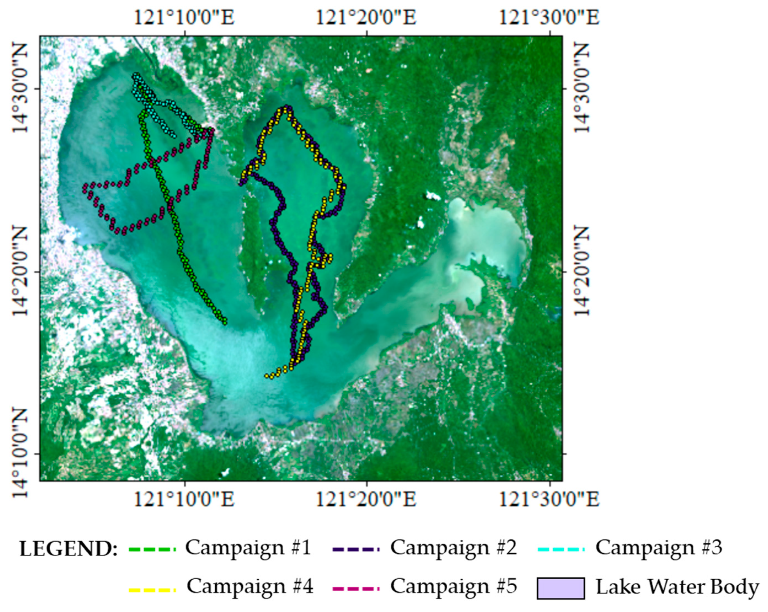
2.1. Laguna Lake of the Philippines
2.2. Lake Victoria of Uganda
2.3. Sentinel-3 Image Dataset
3. Methodology
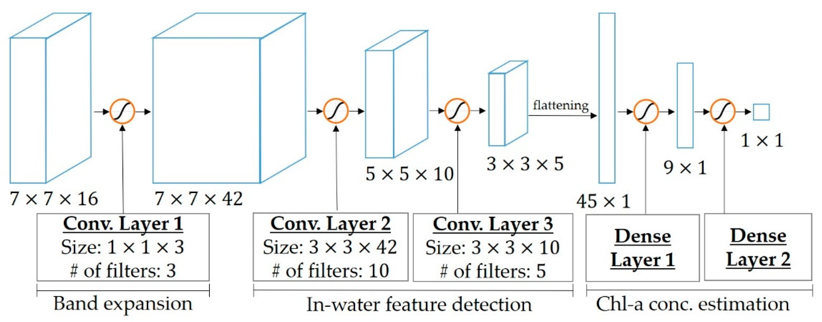
3.1. Artificial Neural Network Model
3.2. ANN Model Training
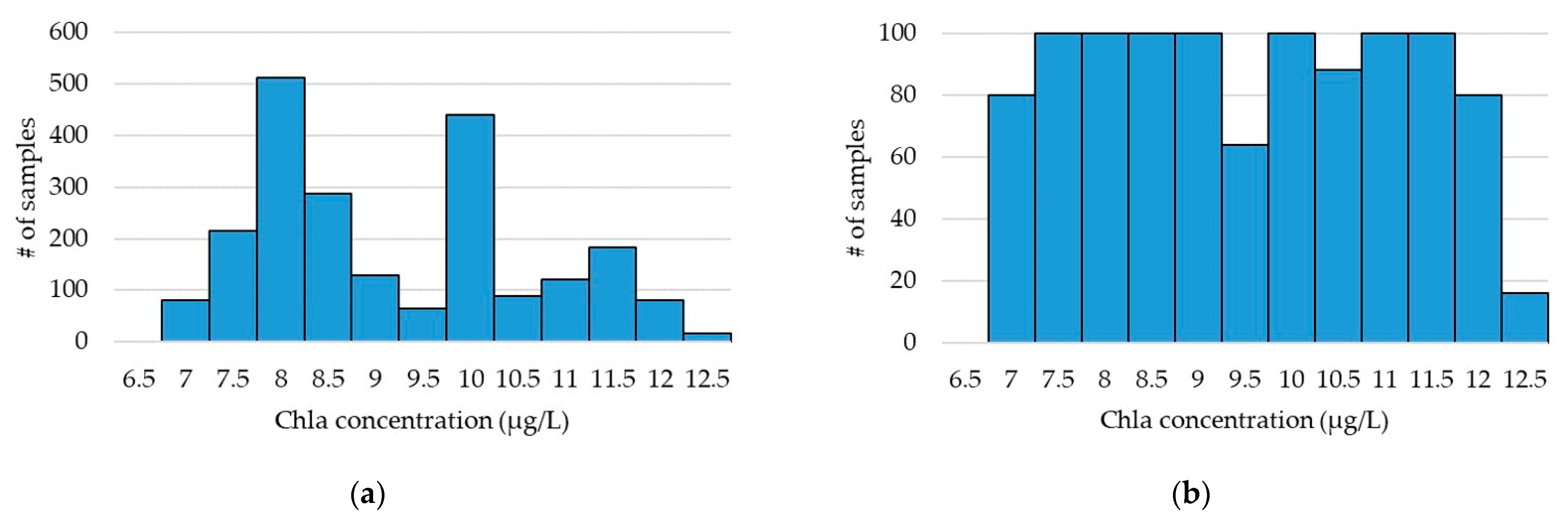
3.2.1. Data Augmentation and Rebalancing
- ■
- The simulated labelled data ,
- ■
- the in situ labelled data which also refer to the original dataset
- ■
- the augmented dataset , and
- ■
- the rebalanced dataset .
3.2.2. Transfer Learning
- Main-training stage. With the help of the pretraining stage, the ANN model contains suitable values of unknown parameters. Training them with the rebalanced dataset increases the possibility that the search for the global minimum in the loss function can be reached. This also means that the accuracy of the estimation is enhanced or the estimation error is smaller. The error is then backpropagated to update the unknown parameters and the spatial feature is more robust.
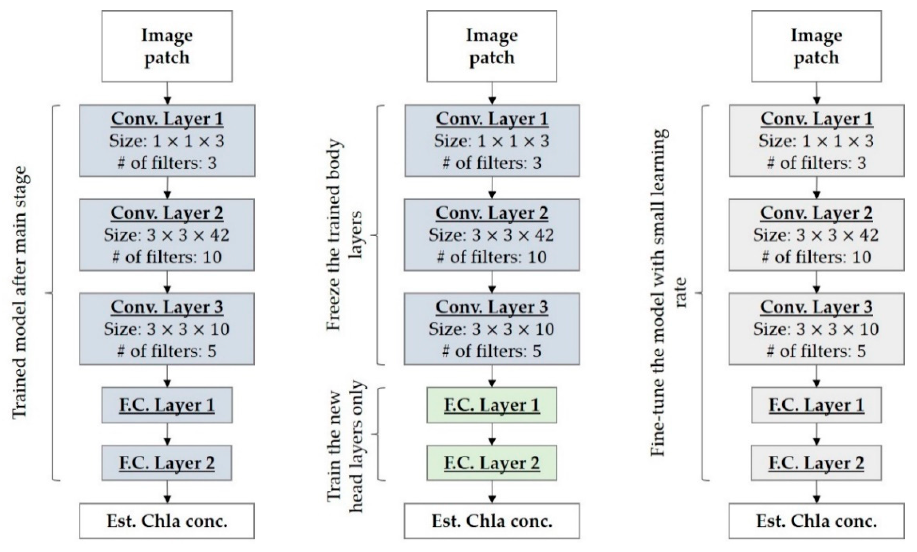
- Fine-tuning stage. In the previous stage, the extraction of the spatial feature is already powerful, and continuing training the previously trained ANN model with the rebalanced dataset may only endanger the spatial feature. Therefore, a fine-tuning technique is performed in this stage by means of “network surgery”. First, the model is split into two parts: the body part, consisting of the first and second phase of the ANN model; and the head part, consisting of the last phase of the ANN model, which is the Chla concentration estimation phase. The head part is then removed, leaving the body part only. Inputting an image patch to the body part only will result in a spatial feature image. In machine learning, the technique to split and remove the head part is known as a feature extractor. Moreover, a new head part containing a similar network as the last phase with a random initial value for the unknown parameters is attached to the body part. Here, if the gradient is allowed to backpropagate from these random values all the way through the network, the powerful spatial features could be at risk. To prevent this problem, the layers in the body part, i.e., in the first and second phase of the model, are frozen or set as untrainable and allow the backpropagation when training be performed on the new head only. This allows the network to start learning from the powerful spatial feature and the estimation of Chla concentration can be optimized. Lastly, all of the layers are unfrozen or set as trainable. However, different to the previous stage or sub-stage in which the training is conducted with a learning rate of 0.001, the learning rate is now set to a very small rate of 0.0001. The aim of setting such very small rate is to obtain a suitable adjustment for the body and head parts. For simplification, Figure 5 shows the workflow of the fine-tuning stage.
4. Experimental Results and Discussion
4.1. Evaluation of the Transfer Learning
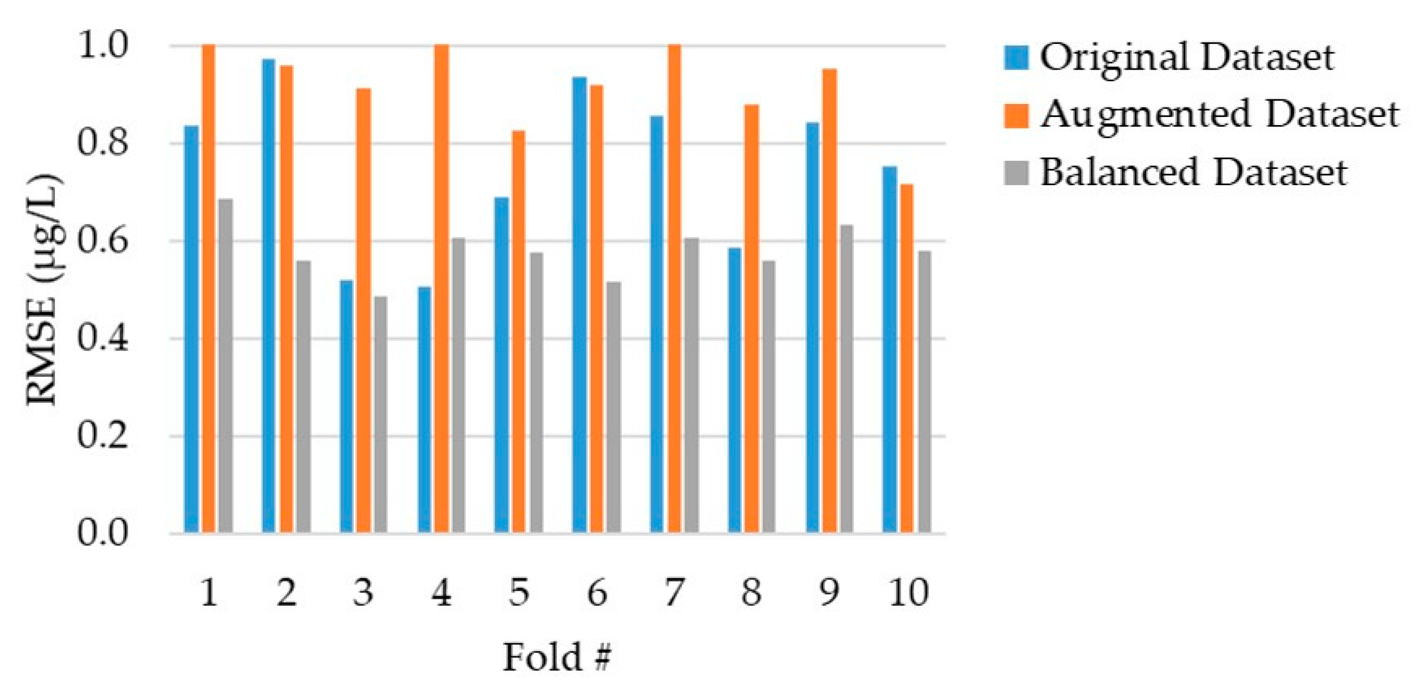
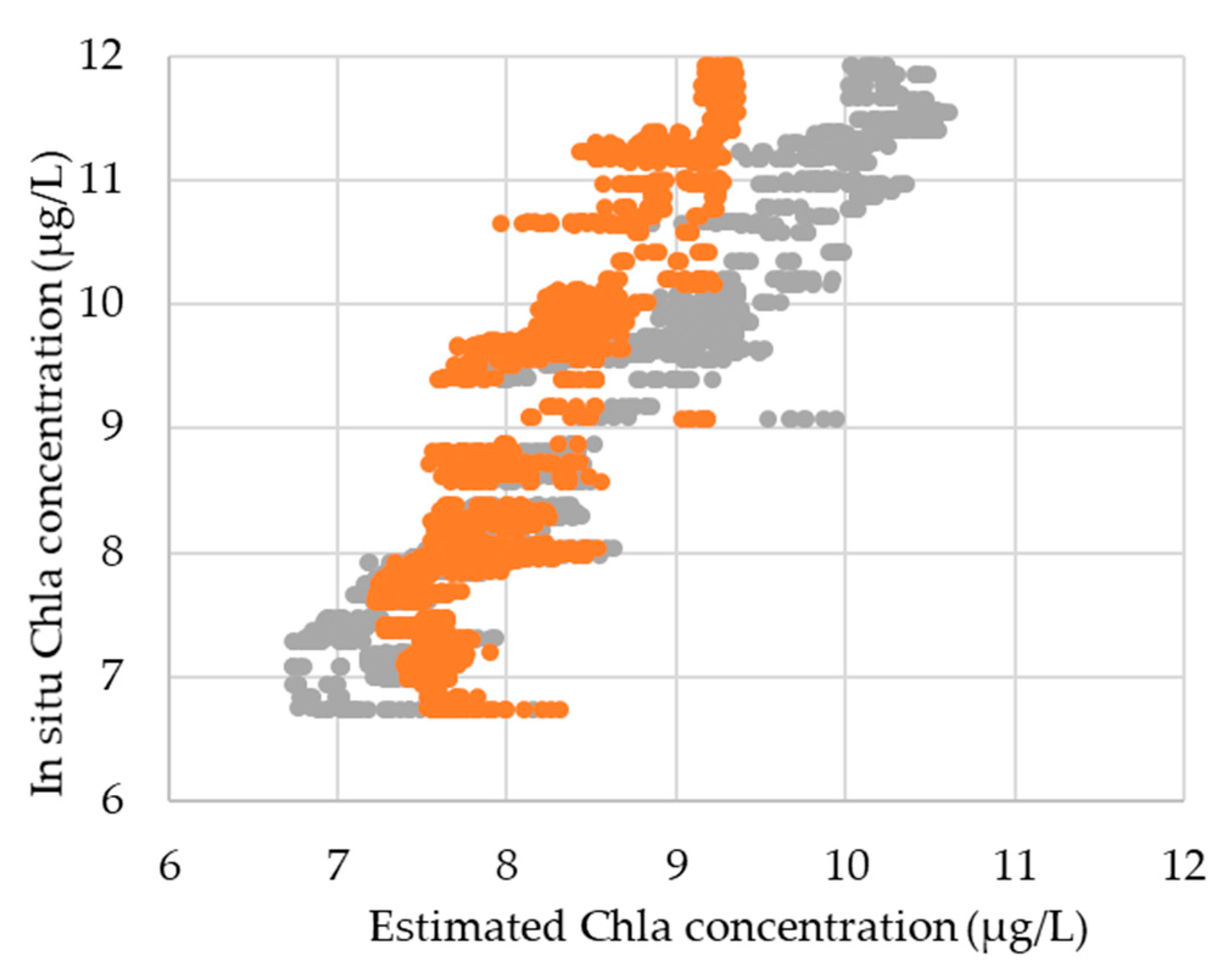
4.2. Performance of Data Augmentation and Rebalancing
4.3. Comparisons of Chla Estimation Models
5. Conclusions and Future Work
Author Contributions
Funding
Institutional Review Board Statement
Informed Consent Statement
Data Availability Statement
Acknowledgments
Conflicts of Interest
References
- Kira, T.; Ide, S.; Fukada, F.; Nakamura, M. Lake Biwa Experience and Lessons Learned Brief. In Managing Lakes and Their Basins for Sustainable Use: A Report for Lake Basin Manegers and Stakeholders; International Lake Environment Committee: Otsu, Japan, 2006; Volume 5. [Google Scholar]
- Kementerian Lingkungan Hidup. Profil 15 Danau Prioritas Indonesia; Kementerian Lingkungan Hidup: Jakarta, Indonesia, 2011.
- Ipsos Business Consultant. Indonesia’s Aquaculture-Key Sectors for Future Growth; Ipsos Business Consultant: Jakarta, Indonesia, 2010. [Google Scholar]
- World Bank. Fish to 2030 Prospects for Fisheries and Aquaculture; World Bank: Washington, DC, USA, 2013. [Google Scholar]
- Cristina, S.; Fragoso, B.; Icely, J.; Grant, J. Aquaspace Project Document; Aquaspace Project: Sagaremisco, Portugal, 2018. [Google Scholar]
- Gurlin, D.; Gitelson, A.A.; Moses, W.J. Remote estimation of chl-a concentration in turbid productive waters-Return to a simple two-band NIR-red model? Remote Sens. Environ. 2011, 115, 3479–3490. [Google Scholar] [CrossRef]
- Moutzouris-Sidiris, I.; Topouzelis, K. Assessment of Chlorophyll-a concentration from Sentinel-3 satellite images at the Mediterranean Sea using CMEMS open source in situ data. Open Geosci. 2021, 13, 85–97. [Google Scholar] [CrossRef]
- Carlson, R.E. A trophic state index for lakes. Limnol. Oceanogr. 1977, 22, 361–369. [Google Scholar] [CrossRef] [Green Version]
- Dall’Olmo, G.; Gitelson, A.A. Effect of bio-optical parameter variability and uncertainties in reflectance measurements on the remote estimation of chlorophyll-a concentration in turbid productive waters: Modeling results. Appl. Opt. 2006, 45, 3577. [Google Scholar] [CrossRef] [PubMed] [Green Version]
- Al Shehhi, M.R.; Gherboudj, I.; Zhao, J.; Ghedira, H. Improved atmospheric correction and chlorophyll-a remote sensing models for turbid waters in a dusty environment. ISPRS J. Photogramm. Remote Sens. 2017, 133, 46–60. [Google Scholar] [CrossRef]
- Chen, J.; Zhang, X.; Quan, W. Retrieval chlorophyll-a concentration from coastal waters: Three-band semi-analytical algorithms comparison and development. Opt. Express 2013, 21, 9024. [Google Scholar] [CrossRef]
- Gitelson, A.A.; Dall’Olmo, G.; Moses, W.; Rundquist, D.C.; Barrow, T.; Fisher, T.R.; Gurlin, D.; Holz, J. A simple semi-analytical model for remote estimation of chlorophyll-a in turbid waters: Validation. Remote Sens. Environ. 2008, 112, 3582–3593. [Google Scholar] [CrossRef]
- Moses, W.J.; Gitelson, A.A.; Berdnikov, S.; Povazhnyy, V. Satellite estimation of chlorophyll-a concentration using the red and NIR bands of MERIS-The azov sea case study. IEEE Geosci. Remote Sens. Lett. 2009, 6, 845–849. [Google Scholar] [CrossRef]
- Mishra, S.; Mishra, D.R. Normalized difference chlorophyll index: A novel model for remote estimation of chlorophyll-a concentration in turbid productive waters. Remote Sens. Environ. 2012, 117, 394–406. [Google Scholar] [CrossRef]
- Andrzej Urbanski, J.; Wochna, A.; Bubak, I.; Grzybowski, W.; Lukawska-Matuszewska, K.; Łącka, M.; Śliwińska, S.; Wojtasiewicz, B.; Zajączkowski, M. Application of Landsat 8 imagery to regional-scale assessment of lake water quality. Int. J. Appl. Earth Obs. Geoinf. 2016, 51, 28–36. [Google Scholar] [CrossRef]
- Niroumand-jadidi, M.; Bovolo, F.; Bruzzone, L. Novel Spectra-Derived Features for Empirical Retrieval of Water Quality Parameters: Demonstrations for OLI, MSI. IEEE Trans. Geosci. Remote Sens. 2019, 57, 10285–10300. [Google Scholar] [CrossRef]
- Van Nguyen, M.; Lin, C.H.; Chu, H.J.; Jaelani, L.M.; Syariz, M.A. Spectral feature selection optimization for water quality estimation. Int. J. Environ. Res. Public Health 2020, 17, 272. [Google Scholar] [CrossRef] [PubMed] [Green Version]
- Wang, X.; Zhang, F.; Ding, J. Evaluation of water quality based on a machine learning algorithm and water quality index for the Ebinur Lake Watershed. Sci. Rep. 2017, 7, 12858. [Google Scholar] [CrossRef] [PubMed] [Green Version]
- Zhang, Y.; Feng, X.; Cheng, X.; Wang, C. Remote estimation of chlorophyll-a concentrations in Taihu Lake during cyanobacterial algae bloom outbreak. In Proceedings of the 2011 19th International Conference on Geoinformatics, Shanghai, China, 24–26 June 2011; pp. 1–6. [Google Scholar]
- Guo, Y.; Liu, C.; Ye, R.; Duan, Q. Advances on water quality detection by uv-vis spectroscopy. Appl. Sci. 2020, 10, 6874. [Google Scholar] [CrossRef]
- Buckton, D.; O’Mongain, E.; Danaher, S. The use of Neural Networks for the estimation of oceanic constituents based on the MERIS instrument. Int. J. Remote Sens. 1999, 20, 1841–1851. [Google Scholar] [CrossRef]
- Kown, Y.S.; Baek, S.H.; Lim, Y.K.; Pyo, J.C.; Ligaray, M.; Park, Y.; Cho, K.H. Monitoring coastal chlorophyll-a concentrations in coastal areas using machine learning models. Water 2018, 10, 1020. [Google Scholar] [CrossRef] [Green Version]
- Samli, R.; Sivri, N.; Sevgen, S.; Kiremitci, V.Z. Applying artificial neural networks for the estimation of chlorophyll-a concentrations along the Istanbul coast. Pol. J. Environ. Stud. 2014, 23, 1281–1287. [Google Scholar]
- Wang, Q.; Wang, S. A predictive model of chlorophyll a in western lake erie based on artificial neural network. Appl. Sci. 2021, 11, 6529. [Google Scholar] [CrossRef]
- Hafeez, S.; Wong, M.; Ho, H.; Nazeer, M.; Nichol, J.; Abbas, S.; Tang, D.; Lee, K.; Pun, L. Comparison of Machine Learning Algorithms for Retrieval of Water Quality Indicators in Case-II Waters: A Case Study of Hong Kong. Remote Sens. 2019, 11, 617. [Google Scholar] [CrossRef] [Green Version]
- Aptoula, E.; Ariman, S. Chlorophyll-a Retrieval From Sentinel-2 Images Using Convolutional Neural Network Regression. IEEE Geosci. Remote Sens. Lett. 2021, 20, 1–5. [Google Scholar] [CrossRef]
- Choi, J.H.; Kim, J.; Won, J.; Min, O. Modelling Chlorophyll-a Concentration using Deep Neural Networks considering Extreme Data Imbalance and Skewness. In Proceedings of the 2019 21st International Conference on Advanced Communication Technology (ICACT), Pyeongchang, Korea, 17–20 February 2019; pp. 631–634. [Google Scholar]
- Pyo, J.C.; Duan, H.; Baek, S.; Kim, M.S.; Jeon, T.; Kwon, Y.S.; Lee, H.; Cho, K.H. A convolutional neural network regression for quantifying cyanobacteria using hyperspectral imagery. Remote Sens. Environ. 2019, 233, 111350. [Google Scholar] [CrossRef]
- Syariz, M.A.; Lin, C.; Blanco, A.C. Chlorophyll-a Concentration Retrieval using Convolutional Neural Networks in Laugna Lake, Philippines. Int. Arch. Photogramm. Remote Sens. Spat. Inf. Sci. 2019, 42, 14–15. [Google Scholar]
- Van Nguyen, M.; Lin, C.; Syariz, M.A.; Thu, T.; Le, H.; Blanco, A.C. Multi-task Convolution Neural Network for Season-insensitive Chlorophyll-a Estimation in Inland Water. IEEE J. Sel. Top. Appl. Earth Obs. Remote Sens. 2021, 14, 10439–10449. [Google Scholar] [CrossRef]
- Ioannou, I.; Gilerson, A.; Gross, B.; Moshary, F.; Ahmed, S. Deriving ocean color products using neural networks. Remote Sens. Environ. 2013, 134, 78–91. [Google Scholar] [CrossRef]
- Ioannou, I.; Gilerson, A.; Gross, B.; Moshary, F.; Ahmed, S. Neural network approach to retrieve the inherent optical properties of the ocean from observations of MODIS. Appl. Opt. 2011, 50, 3168. [Google Scholar] [CrossRef]
- Yu, B.; Xu, L.; Peng, J.; Hu, Z. Global chlorophyll-a concentration estimation from moderate resolution imaging spectroradiometer using convolutional neural networks. J. Appl. Remote Sens. 2021, 14, 034520. [Google Scholar] [CrossRef]
- Syariz, M.A.; Lin, C.H.; Van Nguyen, M.; Jaelani, L.M.; Blanco, A.C. WaterNet: A convolutional neural network for chlorophyll-a concentration retrieval. Remote Sens. 2020, 12, 1966. [Google Scholar] [CrossRef]
- Saguin, K. Biographies of fish for the city: Urban metabolism of Laguna Lake aquaculture. Geoforum 2014, 54, 28–38. [Google Scholar] [CrossRef]
- Herrera, E.; Nadaoka, K.; Blanco, A.C.; Hernandez, E.C. Hydrodynamic investigation of a shallow lake environment (Laguna Lake, Philippines) and associated implications for eutrophic vulnerability. ASEAN Eng. J. Part C 2015, 4, 48–62. [Google Scholar]
- Tamayo-Zafaralla, M.; Santos, R.A.V.; Orozco, R.P.; Elegado, G.C.P. The ecological status of Lake Laguna de Bay, Philippines. Aquat. Ecosyst. Health Manag. 2002, 5, 127–138. [Google Scholar] [CrossRef]
- Deirmendjian, L.; Lambert, T.; Morana, C. Dissolved organic matter composition and reactivity in Lake Victoria, the World’s largest tropical lake. Biogeochemistry 2020, 150, 61–83. [Google Scholar] [CrossRef]
- European Space Agency. Copernicus Sentinel-3 OLCI Land User Handbook; European Space Agency: Paris, France, 2021. [Google Scholar]
- Bricaud, A.; Morel, A.; Babin, M.; Allali, K.; Claustre, H. Variations of light absorption by suspended particles with chlorophyll a concentration in oceanic (case 1) waters: Analysis and implications for bio-optical models. J. Geophys. Res. 1998, 103, 31033–31044. [Google Scholar] [CrossRef]
- Ha, N.T.T.; Koike, K.; Nhuan, M.T.; Canh, B.D.; Thao, N.T.P.; Parsons, M. Landsat 8/OLI Two bands ratio algorithm for chlorophyll-a concentration mapping in hypertrophic waters: An application to west lake in Hanoi (Vietnam). IEEE J. Sel. Top. Appl. Earth Obs. Remote Sens. 2017, 10, 4919–4929. [Google Scholar] [CrossRef]
- Ha, N.T.T.; Koike, K.; Nhuan, M.T. Improved accuracy of chlorophyll-a concentration estimates from MODIS Imagery using a two-band ratio algorithm and geostatistics: As applied to the monitoring of eutrophication processes over Tien Yen Bay (Northern Vietnam). Remote Sens. 2013, 6, 421–442. [Google Scholar] [CrossRef] [Green Version]
- Menon, H.B.; Adhikari, A. Remote Sensing of Chlorophyll-A in Case II Waters: A Novel Approach With Improved Accuracy Over Widely Implemented Turbid Water Indices. J. Geophys. Res. Ocean. 2018, 123, 8138–8158. [Google Scholar] [CrossRef]
- Kohl, S.A.A.; Romera-Paredes, B.; Meyer, C.; De Fauw, J.; Ledsam, J.R.; Maier-Hein, K.H.; Ali Eslami, S.M.; Rezende, D.J.; Ronneberger, O. A probabilistic U-net for segmentation of ambiguous images. arxiv 2018, arXiv:1806.05034. [Google Scholar]
- Patterson, J.; Gibson, A. Deep Learning: A Practitioner’s Approach; O’Reilly Media: Sebastopol, CA, USA, 2017; ISBN 9781491914250. [Google Scholar]
- Kingma, D.P.; Ba, J. Adam: A Method for Stochastic Optimization. In Proceedings of the ICLR, San Diego, CA, USA, 7–9 May 2015; pp. 1–15. [Google Scholar]


| Trophic Class | Chla Concentration Range (in μg/L) | Water Condition |
|---|---|---|
| Oligotrophic | 0~2.6 | A lake with very clear waters and high drinking water quality due to low nutrient content and algal production. |
| Mesotrophic | 2.6~20 | Commonly clear water lakes with beds of submerged aquatic plants and medium levels of nutrients. |
| Eutrophic | 20~56 | The water body will be dominated either by aquatic plants or algae. |
| Hypertrophic | More than 56 | Highly nutrient-rich lakes characterized by frequent and severe nuisance algal blooms and low transparency. |
| Campaign # | Date (in 2019) | # of Samples | Chla Concentration Statistics (μg/L) | |||
|---|---|---|---|---|---|---|
| Min. | Max. | Mean | Std. | |||
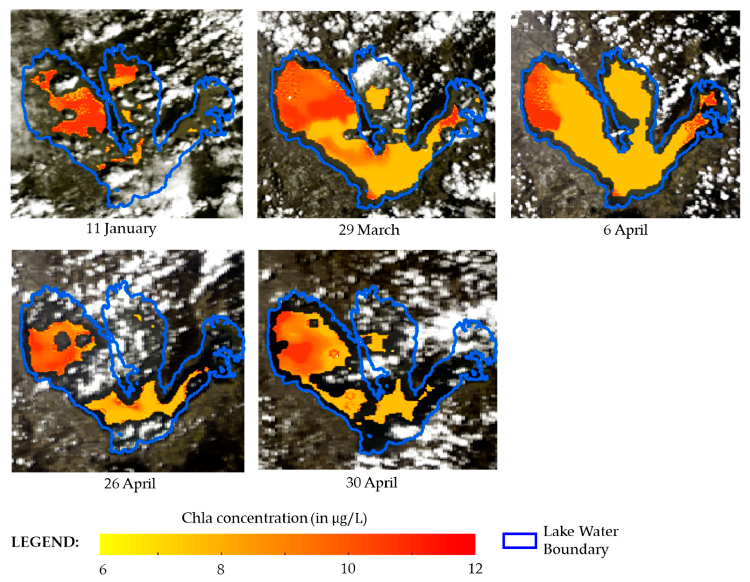
| 1 | 11 Jan | 35 | 9.072 | 13.235 | 11.391 | 0.655 |
| 2 | 29 Mar | 74 | 7.378 | 8.076 | 7.906 | 0.163 |
| 3 | 6 Apr | 98 | 6.980 | 10.970 | 8.459 | 1.218 |
| 4 | 26 Apr | 22 | 6.731 | 7.692 | 7.254 | 0.315 |
| 5 | 30 Apr | 48 | 7.856 | 11.295 | 9.613 | 0.801 |
| Image Acquisition Day | # of Image Patches | |
|---|---|---|
| Pretraining Stage | Transfer-Learning Stage | |
| 11 Jan | 1008 | 35 |
| 29 Mar | 4715 | 74 |
| 6 Apr | 5681 | 98 |
| 26 Apr | 1908 | 22 |
| 30 Apr | 2582 | 48 |
| 15 Jan | 3471 | |
| 22 Jan | 2017 | |
| 7 Feb | 3722 | |
| 8 Feb | 3681 | |
| 19 Feb | 2877 | |
| 2 Mar | 1654 | |
| 10 Mar | 3393 | |
| 26 Mar | 2766 | |
| 10 Apr | 3984 | |
| 21 Apr | 3772 | |
| Total | 47,231 | 275 |
| Fold | Transfer Learning Performance (RMSE in μg/L) | ||
|---|---|---|---|
| Pretraining Stage | Transfer-Learning | ||
| Main-Training Stage | Fine-Tuning Stage | ||
| 1 | 2.070 | 0.689 | 0.478 |
| 2 | 2.144 | 0.562 | 0.229 |
| 3 | 2.113 | 0.487 | 0.219 |
| 4 | 2.089 | 0.606 | 0.430 |
| 5 | 2.190 | 0.576 | 0.414 |
| 6 | 2.120 | 0.517 | 0.284 |
| 7 | 2.194 | 0.609 | 0.441 |
| 8 | 2.228 | 0.560 | 0.387 |
| 9 | 2.216 | 0.633 | 0.508 |
| 10 | 2.079 | 0.581 | 0.336 |
| Avg. | 2.144 | 0.582 | 0.372 |
| Model Name | Formula | Calibration Model |
|---|---|---|
| Three-band model | Linear regression | |
| Two-band model | Linear regression | |
| NDCI | ||
| WaterNet |
| Station Name | Estimation Error (in μg/L) | ||||
|---|---|---|---|---|---|
| Three-Band Model | Two-Band Model | NDCI | WaterNet | Proposed Method | |
| LV1 | 0.746 | 0.653 | 0.304 | 0.645 | 0.302 |
| LV2 | 0.367 | 0.303 | −0.164 | 0.277 | 0.117 |
| RMSE | 0.588 | 0.509 | 0.244 | 0.496 | 0.229 |
Publisher’s Note: MDPI stays neutral with regard to jurisdictional claims in published maps and institutional affiliations. |
© 2021 by the authors. Licensee MDPI, Basel, Switzerland. This article is an open access article distributed under the terms and conditions of the Creative Commons Attribution (CC BY) license (https://creativecommons.org/licenses/by/4.0/).
Share and Cite
Syariz, M.A.; Lin, C.-H.; Heriza, D.; Lasminto, U.; Sukojo, B.M.; Jaelani, L.M. A Transfer Learning Technique for Inland Chlorophyll-a Concentration Estimation Using Sentinel-3 Imagery. Appl. Sci. 2022, 12, 203. https://doi.org/10.3390/app12010203
Syariz MA, Lin C-H, Heriza D, Lasminto U, Sukojo BM, Jaelani LM. A Transfer Learning Technique for Inland Chlorophyll-a Concentration Estimation Using Sentinel-3 Imagery. Applied Sciences. 2022; 12(1):203. https://doi.org/10.3390/app12010203
Chicago/Turabian StyleSyariz, Muhammad Aldila, Chao-Hung Lin, Dewinta Heriza, Umboro Lasminto, Bangun Muljo Sukojo, and Lalu Muhamad Jaelani. 2022. "A Transfer Learning Technique for Inland Chlorophyll-a Concentration Estimation Using Sentinel-3 Imagery" Applied Sciences 12, no. 1: 203. https://doi.org/10.3390/app12010203
APA StyleSyariz, M. A., Lin, C.-H., Heriza, D., Lasminto, U., Sukojo, B. M., & Jaelani, L. M. (2022). A Transfer Learning Technique for Inland Chlorophyll-a Concentration Estimation Using Sentinel-3 Imagery. Applied Sciences, 12(1), 203. https://doi.org/10.3390/app12010203