Solar Irradiance Forecasting Using a Data-Driven Algorithm and Contextual Optimisation

Abstract

Solar forecasting plays a key part in the renewable energy transition. Major challenges, related to load balancing and grid stability, emerge when a high percentage of energy is provided by renewables. These can be tackled by new energy management strategies guided by power forecasts. This paper presents a data-driven and contextual optimisation forecasting (DCF) algorithm for solar irradiance that was comprehensively validated using short- and long-term predictions, in three US cities: Denver, Boston, and Seattle. Moreover, step-by-step implementation guidelines to follow and reproduce the results were proposed. Initially, a comparative study of two machine learning (ML) algorithms, the support vector machine (SVM) and Facebook Prophet (FBP) for solar prediction was conducted. The short-term SVM outperformed the FBP model for the 1- and 2- hour prediction, achieving a coefficient of determination (R²) of 91.2% in Boston. However, FBP displayed sustained performance for increasing the forecast horizon and yielded better results for 3-hour and long-term forecasts. The algorithms were optimised by further contextual model adjustments which resulted in substantially improved performance. Thus, DCF utilised SVM for short-term and FBP for long-term predictions and optimised their performance using contextual information. DCF achieved consistent performance for the three cities and for long- and short-term predictions, with an average R² of 85%.

1. Introduction

Greenhouse gases are major drivers of climate change [1] and are primarily produced by energy generation from fossil fuels [2]. Substantial research and political attention have been devoted to renewable energies in order to reduce the consumption of fossil fuels [3]. According to Huybrechts [4], renewable solar energy generation has continuously increased in the context of attempts to transition to a net-zero carbon economy, as shown in Figure 1. However, major challenges arise when a higher percentage of renewable energy is connected to the grid, due to its volatile nature [5]. If supply and demand are not of a similar magnitude, energy grids become unstable, potentially leading to blackouts [6]. Load balancing, ensuring that equal amounts of energy are generated and consumed, is one of the most important and difficult of these challenges [7]. This has conventionally been achieved by adjusting energy generation to demand patterns and scaling up power generation whenever necessary. Currently, the backup capacity for load balancing is mostly provided by fossil fuels, generation of which can be ramped up on demand [8].

Renewable energy depends on environmental factors [10,11], and is, therefore, harder to match to demand patterns. This stipulates the need for appropriate energy management, including the organisation of generation, storage, and consumption. Understanding energy generation patterns plays a key part in developing effective management strategies. Therefore, the prediction of renewable power output is necessary to integrate more renewable energy into the grid and thus reduce the emission of greenhouse gases [12].

In order to forecast the power output of any solar technology, the amount of available potential energy must be known. If prediction models are specific to one type of device, it is harder to adapt them to other use cases. The potential energy generated by many technologies, e.g., PV panels, depends on the amount of solar global horizontal irradiance received at a certain location. Global horizontal irradiance is the sum of direct and diffuse radiation on a horizontal plane and is also used to calculate the radiation on an inclined plane, such as a solar panel [13]. The prediction of solar radiation allows us to infer the power output of devices, such as photovoltaic cells or solar water heaters. Throughout this paper, global horizontal irradiance will also be referred to as simply irradiance or radiation.

In recent years, solar prediction in particular has become more sophisticated. Much of this advancement is attributed to the development of machine learning (ML) algorithms [14]. There has been a tremendous increase in the use of ML for solar predictions in the last decade. It has been successfully employed and is extensively discussed in review papers by Sobri et al. [12] and Wang et al. [14]. This paper builds on these insights and proposes a forecasting algorithm that predicts solar irradiance using ML algorithms and contextual optimisation.

Motivations and Impact

The need for ML-driven energy management solutions is increasing with the net-zero carbon by 2050 target set by the UK government [15]. Several contributing parameters to managing energy in our society include demand, energy usage behaviour, environmental factors, etc. In this paper, we addressed the question of how to accurately forecast solar irradiance. This plays a crucial role in choosing the most optimal energy system management strategy, and optimising the integration of solar cells [16]. Moreover, we aim to present a methodological foundation of algorithm and feature selection, and evaluation metrics for other studies to follow.

The main contributions of this paper are as follows:

• Data-driven and contextual optimisation forecasting (DCF) algorithm, which accurately predicts solar irradiance in the short- and long term. DCF is a hybrid algorithm that utilises state-of-the-art ML algorithms and optimises their accuracy using contextual information;
• A comparative study of two ML algorithms (Support Vector Machine and Facebook Prophet), in which an investigation was made into the effect of adding extraterrestrial radiation as a feature;
• Comprehensive validation of the forecasting accuracy for short- and long-term predictions in three cities to ensure that the model is not specific to one location. This was evaluated by computing the coefficient of determination (R²), mean absolute error (MAE), and root-mean-squared error (RMSE).

The rest of the paper is organised as follows: Section 2 reviews previously proposed algorithms for solar forecasting. Section 3 presents the dataset used for training the ML algorithms and the evaluation methods, respectively. The DCF algorithm is introduced in Section 4, while Section 5 discusses the forecasting results. Finally, Section 6 concludes this paper, and Section 7 suggests potential future research.

2. Literature Review

There is a range of ML algorithms that have been used in solar irradiance prediction, such as regression, Markov chain [17], autoregressive integrated moving average (ARIMA) [18], and neural networks [19]. One of the most commonly used ML algorithms is the support vector machine (SVM) [12,20,21,22]. The SVM model is a conventional algorithm that has been used for more than a decade to predict solar irradiance [21]. There are several advantages to using an SVM; for example, it is able to model complex nonlinear models with considerably high accuracy and robustness, and it is usually immune to overfitting. Furthermore, there are novel algorithms, which are not yet established in solar prediction but have the potential to increase forecasting accuracy, such as the Facebook Prophet (FBP) algorithm. FBP was proposed for forecasting time series where nonlinear trends fit with yearly, weekly, and daily seasonality. It achieves high accuracy with time series that have strong seasonal effects and several seasons of historical data. Additionally, it is robust in handling missing data and shifts in the trend and typically reduces the effect of outliers as shown in Section 2.2.

2.1. Support Vector Machines

SVM is a statistical learning algorithm originally designed for classifying data [23]. It can also be used for regression tasks such as predicting solar radiation [24]. A kernel function transforms a nonlinear input space into a higher-dimensional space [25]. It allows efficient computation of the scalar products of multiple vectors in this higher-dimensional space. Common kernel functions include the polynomial, radial basis (RBF), and sigmoid functions [21]. In the higher-dimensional space, the optimal hyperplane, which separates the margins of errors in regression and classes in classification, can be identified.

The use of SVMs in renewable forecasting has increased drastically in recent years [21]. The SVM is an established method, used across the renewable energy sector, especially for solar forecasting, because of its accurate prediction ability for nonlinear data. Further advantages include its fast computational speed, as no iterative tuning is required, and its capability to produce accurate predictions with a small volume of data [26]. SVMs solve a convex programming problem resulting in the global optimum, avoiding being trapped in local optima (local optimum is either the highest or lowest point, compared with nearby data points. The global optimum is the highest or lowest point in the whole function or dataset. Further reading on convex optimisation problems can be found in [27]).

Zeng and Qiao proposed a least-square SVM to forecast global horizontal irradiance for 1-, 2- and 3-hour ahead [28]. Their model significantly outperformed an autoregressive (AR) model, as well as a radial basis function neural network. However, their evaluation was performed for a short period (10 days) without cross-validating the model performance. VanDeventer et al. developed an SVM model in hybrid with a genetic algorithm to forecast the power output of residential PV systems [29]. The model demonstrated good adaptability to different locations, weather patterns, and climatic conditions. As, PV power output depends on the system parameters and technologies, prediction of the power source (irradiance) is more useful in the long term. An SVM with radial basis function to global solar irradiance in a single location (Tehran) was used by Ramedani et al. [25]. The radial basis function was chosen because it outperformed the polynomial as a kernel function. Furthermore, it outperforms an ANN in terms of root-mean-squared error (RMSE) while being computationally more efficient.

2.2. Facebook Prophet

Facebook Prophet (FBP) is a decomposable time series model, based on additive modelling [30]. Recently, it has gained significant attention due to its capability to accurately forecast time series data. For instance, Lim et al. compared FBP to autoregressive integrated moving average (SARIMA) and concluded that FBP outperformed SARIMA for the prediction of electricity and natural gas demand [31]. Additionally, Shawon et al. predicted PV short circuit current for the next day, deeming it to be a reliable forecasting method [32].

FBP delivers its peak performance when dealing with a time series with strong seasonal effects [33]. This applies to solar irradiance and is one of the main reasons to believe that this algorithm is suitable for solar irradiance forecasting. However, in the literature, FBP has not yet been utilised for solar irradiance prediction.

FBP models the time series data as follows:

$$y\left(t\right)=g\left(t\right)+s\left(t\right)+h\left(t\right)+{ϵ}_t$$

(1)

where the trend is $g\left(t\right)$, the seasonality is $s\left(t\right)$, and the holidays are $h\left(t\right)$. It is worth mentioning that holidays and weekly trends were not accounted for, as these have no influence on solar irradiance, ${ϵ}_t$ indicates the changes not represented by the model and is assumed to be normally distributed. It has intuitively adaptable parameters, designed to be used by analysts that have domain knowledge rather than statistical expertise. Therefore, it is important to know the characteristics of the subject that is being predicted, in this case, the behaviour of solar radiation.

3. Dataset and Evaluation

3.1. Dataset

The data for this paper were acquired from the National Solar Radiation Database (NSRDB) [34] for solar irradiance values in Denver, Seattle, and Boston, as shown in

Table 1. Datasets are from the National Solar Radiation Database [34].

City	Station Name	ID	Latitude	Longitude
Denver	Denver/Centennial	724666	39.742°	−105.179°
Boston	Boston Logan	725090	42.367°	−71.017°
Seattle	Seattle Seattle-Tacoma	727930	47.46°	122.317°

. These were selected due to their different geographical and meteorological conditions. Thus, the forecasting algorithm would not be specific to one location.

The datasets contained hourly data for 8 years (1998–2005), including global horizontal irradiance and extraterrestrial radiation on a horizontal surface. Extraterrestrial radiation on a horizontal surface is the amount of solar radiation received at the top of the atmosphere on a horizontal surface. This will be referred to as extraterrestrial radiation throughout this paper (this is not to be confused with the solar constant. Further reading on solar radiation can be found in Kalogirou’s book Solar Energy Engineering [35]. These datasets were used to predict hourly values for the global horizontal irradiance.

By averaging every hour of the day over the given 8 years, 1D and 2D plots were created and are shown in Figure 2, respectively. While the 1D plot only captures the seasonal trend, the 2D representation also displays the daily seasonality which depends on the latitude of the location.

3.2. Evaluation

The DCF algorithm was assessed for short- and long-term forecasting. The short-term forecasts for 1-, 2- and 3-hour ahead were generated, as is common in the literature [12,29,36,37]. Forecasts for a few hours ahead help to manage and schedule the start-up of power plants (load scheduling) [37]. Furthermore, short-term forecasts of 30 min to 6 h are important for load dispatch and scheduling [24]. Load dispatch means that electricity can be dispatched on demand, and load scheduling is the management of this electricity and its usage.

The long-term prediction capabilities were investigated by forecasting irradiance data for 1 year (24 × 365 h) ahead. Long-term forecasting of several months up to a year is useful for scheduling maintenance and has value when bidding on the energy market [38]. There are few studies on long-term predictions in the literature using statistical methods [12]. It might relate to the fact that physical models based on meteorological expertise are generally more accurate at predicting long-term solar radiation [39]. The long-term prediction of this ML model does not detect any change in weather and only gives an approximate idea of the radiation values. However, this model is useful, as its implementation is easier and quicker than the implementation of a physical model and still gives a good indication of the amount of radiation that will be received

All models were tested on hourly data for a whole year (2005). These results were affirmed using fivefold cross validation for the SVM model. Cross validation for FBP cannot be performed like common k-fold validation, as the time series should not be randomly separated. Therefore, the 1-, 2-, and 3-hour predictions were made for FBP using every hour of the year as the starting point, thus generating 8760 × 3 forecasts. Based on these predictions and target values, several evaluation metrics were calculated. As for k-fold cross validation, the more starting points there are (the higher the k), the more generalised the result will be.

The forecasting was evaluated and compared using the coefficient of determination (R²), mean absolute error (MAE), and root-mean-squared error (RMSE).

The R² value is obtained as follows [40]:

$$R^2=\frac{{\Sigma }_i\left(y_i-{\widehat{y}}_i\right)}{{\Sigma }_i\left(y_i-{\overline{y}}_i\right)}$$

(2)

where $y_i$ are the actual values,${\overline{y}}_i$ is the mean of the actual values, and ${\widehat{y}}_i$ are the predicted values.

MAE has the same units as the predicted value and thus represents the expected absolute error, which is calculated by [41].

$$MAE=\frac{1}{N} {\displaystyle \sum }_{i=1}^N\left|y_i-{\widehat{y}}_i\right|$$

(3)

where $N$ is the total number of samples.

The RMSE value squares the difference between actual and predicted values, emphasising larger errors. This is appropriate for solar prediction as larger errors lead to disproportionally higher costs [42]. RMSE can be calculated as follows [43]:

$$RMSE=\sqrt{{\displaystyle \sum }_{i=1}^N\frac{{\left(y_i-{\widehat{y}}_i\right)}^2}{N}}$$

(4)

To evaluate the prediction accuracy, the data were trained on radiation data from 1998 to 2004 and tested on data from 2005. Cross validation was performed, showing that the models generalise well. Furthermore, grid search was applied to tune the hyperparameters. After training and making predictions, these were adjusted using contextual optimisation.

4. Data-Driven and Contextual Optimisation Forecasting Algorithm

The DCF algorithm consists of two parts, i.e., data-driven and optimisation using contextual information, as shown in Figure 3. The data-driven part purely depends on the algorithm and the input data, e.g., the selection of the input features. The optimisation part uses contextual information to enhance the forecasting of the data-driven models, such as the elimination of negative predictions. Using this approach, we can harvest the strengths of both machine learning and the contextual understanding of the data.

4.1. Data-Driven Model

In the data-driven part, two promising ML algorithms (SVM and FBP) were utilised to generate the predictions. It was implemented in Python [44] using Scikit-learn [45] and Prophet Libraries [30]. Initially, a comparative study of the SVM and FBP algorithms was conducted to assess their accuracy. Subsequently, the effects of adding extraterrestrial radiation as an input feature to the model were investigated.

For the SVM short-term prediction, three variables were used as initial features, all past values of the global horizontal irradiance. These are the radiation of the same day 1 h ago, the same hour 1 day ago, and the same hour 2 days ago, as shown in

Table 2. Initial and additional features for SVM short- and long-term forecast.

Variable Name	Description
	Short-term Forecast
	Initial Input Features
1H Radiation	Radiation values for the same day 1 h ago
1D Radiation	Radiation values for the same hour 1 day ago
2D Radiation	Radiation values for the same hour 2 days ago
	Additional Input Features
1H Extraterr	Extraterrestrial values for the same day 1 h ago
1D Extraterr	Extraterrestrial values for the same hour 1 day ago
2D Extraterr	Extraterrestrial values for the same hour 2 days ago
	Long-term Forecast
	Initial Input Features
1Y Radiation	Radiation from the same hour and day a year ago
	Additional Input Features
2Y Radiation	Radiation at the same hour and day two years ago
1Y Extraterr	Extraterrestrial radiation of same hour and day a year ago
2Y Extraterr	Extraterrestrial radiation of same hour and day two years ago

. Zeng and Qiao found that the same hour of previous days has a stronger correlation with the target variable than radiation data from 1h ago [28]. For the long-term prediction of the SVM model, radiation values of the same hour and same day one year ago were used as its initial feature (see Table 2), as these have a strong correlation [38].

For the Facebook Prophet short-term prediction, the same variable as for SVM was used, the global horizontal irradiance. However, as FBP has a different algorithm structure, the feature is the time series of solar radiation up to the values that are predicted. There is no differentiation of global horizontal radiation (1H-, 1D-, 2D radiation) as for the SVM model. For example, all values from 00:00 on 1 January 1998 up to 08:00 on 24 June 2005 were used to predict 09:00 + 10:00 + 11:00 on 24 June 2005. Similarly, for the long-term prediction, the entire past time series up to the predicted year was used. The past time series should contain at least one year of data so that seasonalities can be captured. Both the long- and short-term prediction features are shown in

Table 3. Initial and additional features for FBP short- and long-term forecast.

Variable Name	Description
	Short- and Long-term Forecast
	Initial Input Features
Xt=0 … Xt=N	Time series of radiation values from 1 January 1998 to 31 December 2004
	Additional Input Features
Et=0 … Et=N	Time series of extraterrestrial radiation values from 1 January 1998 to 31 December 2004

. These will only differ in their predicted output values (3 h or 1 year).

After choosing the initial features for the data-driven model, further features were added and their effectiveness evaluated. Adding features to a model can improve its performance [28]. However, there is no inherent benefit to increasing the model complexity. Additional features can also lead to worse results or have no impact on performance [46]. Therefore, additional features must be carefully evaluated and only added if shown to have a positive impact.

For the SVM short-term forecast, three inputs were added to the initial features, as shown in Table 2: extraterrestrial radiation for the previous hour of the same day, for the same hour 1 day ago, and for the same hour 2 days prior. For the long-term forecast, the irradiance of the same hour and the same day two years ago, as well as the extraterrestrial radiation were added. The long-term forecast further included the global horizontal irradiance of the same hour and the same day two years ago, as well as the extraterrestrial radiation, as shown in Table 2.

It is only possible to add features to FBP if the future values for these are known. This is not the case for most additional features, such as extraterrestrial radiation. However, extraterrestrial radiation is approximately the same for every time of the year at a given location, so it can be predicted precisely. Thus, a time series of predicted extraterrestrial radiation was added for FBP as additional regressors, for both short- and long-term predictions, as shown in Table 3.

Hyperparameters are different from “normal” parameters, e.g., the weights $\left(\omega \right)$ and biases $\left(b\right)$. They are the parameters that cannot be learned by the SVM model but must be chosen. The hyperparameter were tuned after evaluating the results of the basic algorithm operations for the default values in Scikit-learn. Hyperparameters should be selected to give the best results and can be tuned using several different methods. These include grid search [47], random search [48], and bio-inspired techniques, e.g., swarm optimisation [49].

The hyperparameters for this SVM model were tuned by the grid search cross validation (grid-search cross-validation searches for the best combination of the given parameters using cross validation to evaluate each combination of hyperparameters). For this, a grid of possible hyperparameters was provided. Firstly, the radial basis function (RBF), shown in Equation (5), was chosen, as it produces the best results in the literature [50]. This was verified for these solar models. When using an SVM for regression with an RBF kernel, three parameters must be found: $C$, the regularisation parameter; $\epsilon$, the term defining the size of the error tube; $\gamma$, the width of the RBF kernel.

$$RBF=exp\left(-\gamma \Vert x-{x^{\prime }\Vert }^2\right)$$

(5)

One drawback of grid search cross validation is its computational cost. Other optimisation techniques should be investigated, as discussed in Section 7. To avoid excessive computations, a log-scale was initially used for all hyperparameters, e.g., 0.1, 1, 10, and 100 for $C$. Depending on the outcome, the range was adjusted (e.g., 5, 10, and 50). It was found that $C$ had the greatest influence on the results of this model.

4.2. Contextual Optimisation

The second part of the DCF algorithm optimised the accuracy of the data-driven predictions using the contextual information of solar irradiance. This information was derived from comparing the forecasted values to the measured values, thus not relying on a specific location/time. As shown in Figure 4, optimisation had three steps. It was observed that the data-driven approaches forecasted negative values, so these negative values were eliminated. Then, the forecasted values were amended based on the time of sunrise and sunset, (a similar approach were taken in [19] daytime forecasting). Here, we used two approaches: one static, in which night hours were defined from 8 p.m. to 6 a.m., and one dynamic which determined the hours of sunset and sunrise. The static approach was implanted by Zeng and Quiao, producing good results [28]. The dynamic approach is a more accurate representation of reality and thus can be more flexibly implemented in any location. However, it requires additional computational power. The last step was the seasonal adaptation in which we amended the forecasted values in the long-term model according to the month of the year.

FBP generated large negative values for both long- and short-term predictions. For all negative predictions (which only occurred in winter), the target value was zero. This shows that FBP only forecasted negative values during the night hours, as shown in Figure 5. In summer, all night hour predictions were positive. As there could not be negative irradiance and most negative predictions occurred at night, all negative values were eliminated and set to zero. The SVM model also predicted some negative values (around 5% for short-term and 50% for long-term). For most predictions with negative values, the target value was zero. For the non-zero target values, the radiation was very low (maximum of 15 W/m²). Therefore, here too, all negative values were set to zero.

After eliminating the negative values, all values between 8 pm and 6 am were set to zero, as they were considered night hours [28]. However, this static approach does not represent that sunrise and sunset hours vary over the year. Therefore, the sunset and sunrise for every day of the year were determined and subsequently used to set all values between sunset and sunrise to zero. Both static and dynamic methods were implemented to compare their impact on the model accuracy.

A seasonal adaptation was created for the long-term models, as a general trend was detected. For instance, the long-term FBP model would overpredict in summer and underpredict in winter, especially for the model without extraterrestrial radiation. Further, there was over- and underprediction trends in both seasonal and daily forecasts. For example, in some months, morning and evening hours were underpredicted, while the noon hours were overpredicted, as shown in Figure 6. The seasonal adaptation aimed to prevent these general trends of over- and underpredicting. The model with extraterrestrial radiation displayed less of a yearly seasonal trend; however, the daily trend still existed.

For the seasonal adaptation, for every hour of the day within each month (e.g., the 6th hour of every day in January), all values from previous years were collected. The average of these target values for the particular hour was taken for each month, as shown in Figure 7. The same was carried out for the predicted values. Three different versions of average were used: the mean (V1), the median (V2), and the mean of median and mean (V3).

The seasonal adaptation adjusted the values according to the month of the year by increasing/decreasing every predicted value that was on average lower/higher than the target values of the same hour of the day of that month in past years. The seasonal adaptation (SA) is calculated as follows:

$$\widehat{y}{ }_{SA}=\widehat{y}\times \left(1+\frac{ \overline{y}- \overline{\widehat{y}}}{\overline{\widehat{y}}}\right)$$

(6)

where $\widehat{y}$ refers to the predicted value, y is the target value, and the $\overline{\widehat{y}}$ is the average predicted value. The average here refers to either the mean, median, or mean of median and mean, depending on the version.

In the final DCF, SVM was used for first- and second-hour predictions. Beyond this, FBP would be used as the core algorithm. Furthermore, the best outcome of every comparative step was used. In the data-driven part, extraterrestrial radiation was added as an input feature to the DCF algorithm. The most influential hyperparameter was the regularisation parameter $C$, which was chosen to be 120 for the short-term model and 0.5 for the long-term DCF. In the contextual optimisation, the negative values were eliminated and dynamic sunset- and sunrise adjustments were performed. For the long-term prediction, seasonal adaptation was applied. From the seasonal adaptation variations, V3 (mean of median and mean) was chosen for the SVM model, while V1 (mean) was selected for the FBP. This was verified by the results, presented in Section 5.

5. Results and Discussion

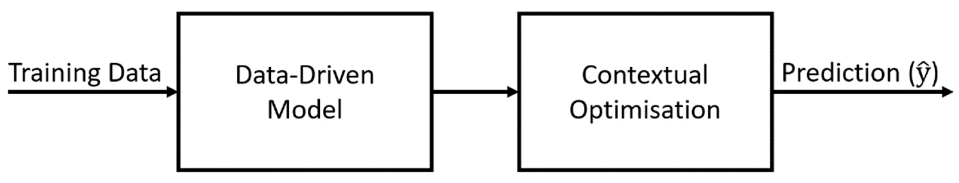
This section consists of three main parts. First, the data-driven part of the model is evaluated, followed by a discussion of the improvements brought about by contextual optimisation. Subsequently, the final DCF model is presented and validated by the short- and long-term models in all three cities.

5.1. Data-Driven Model Results

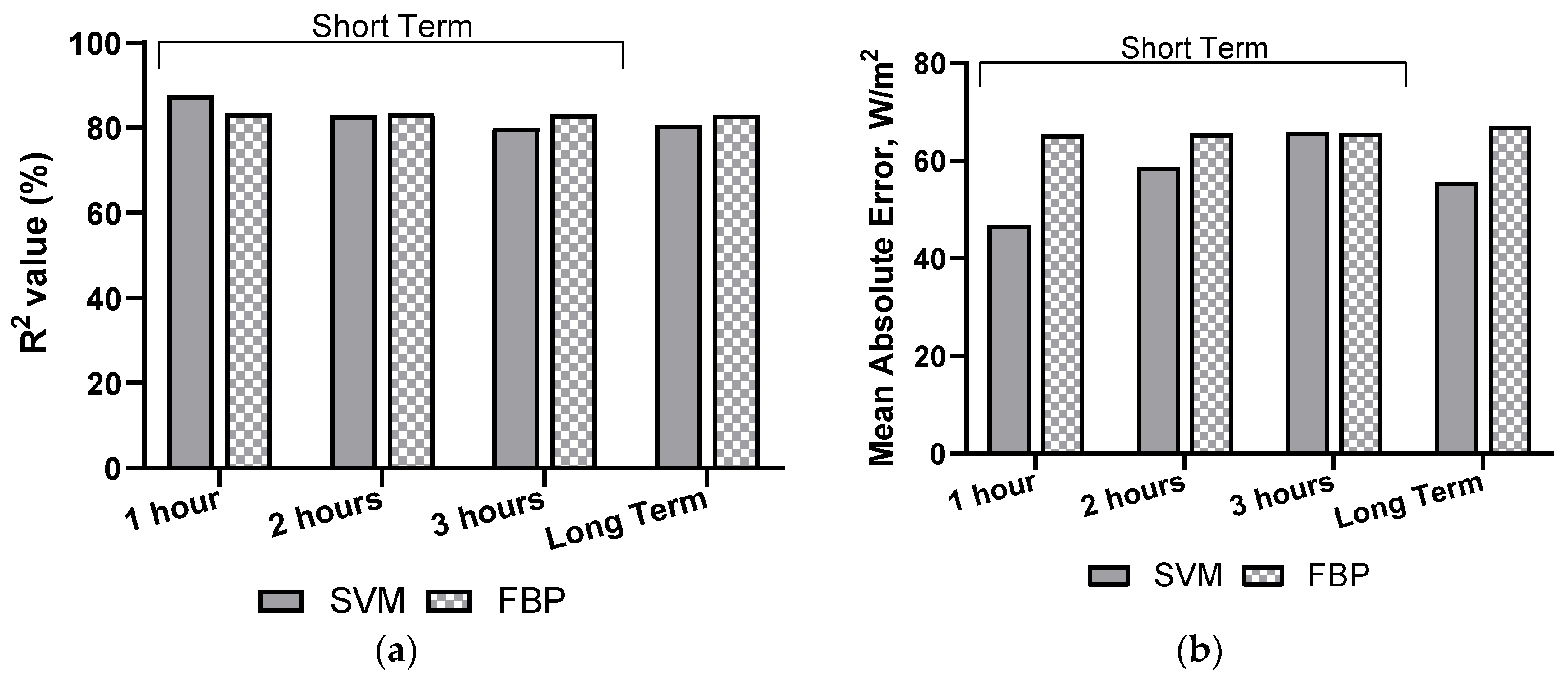
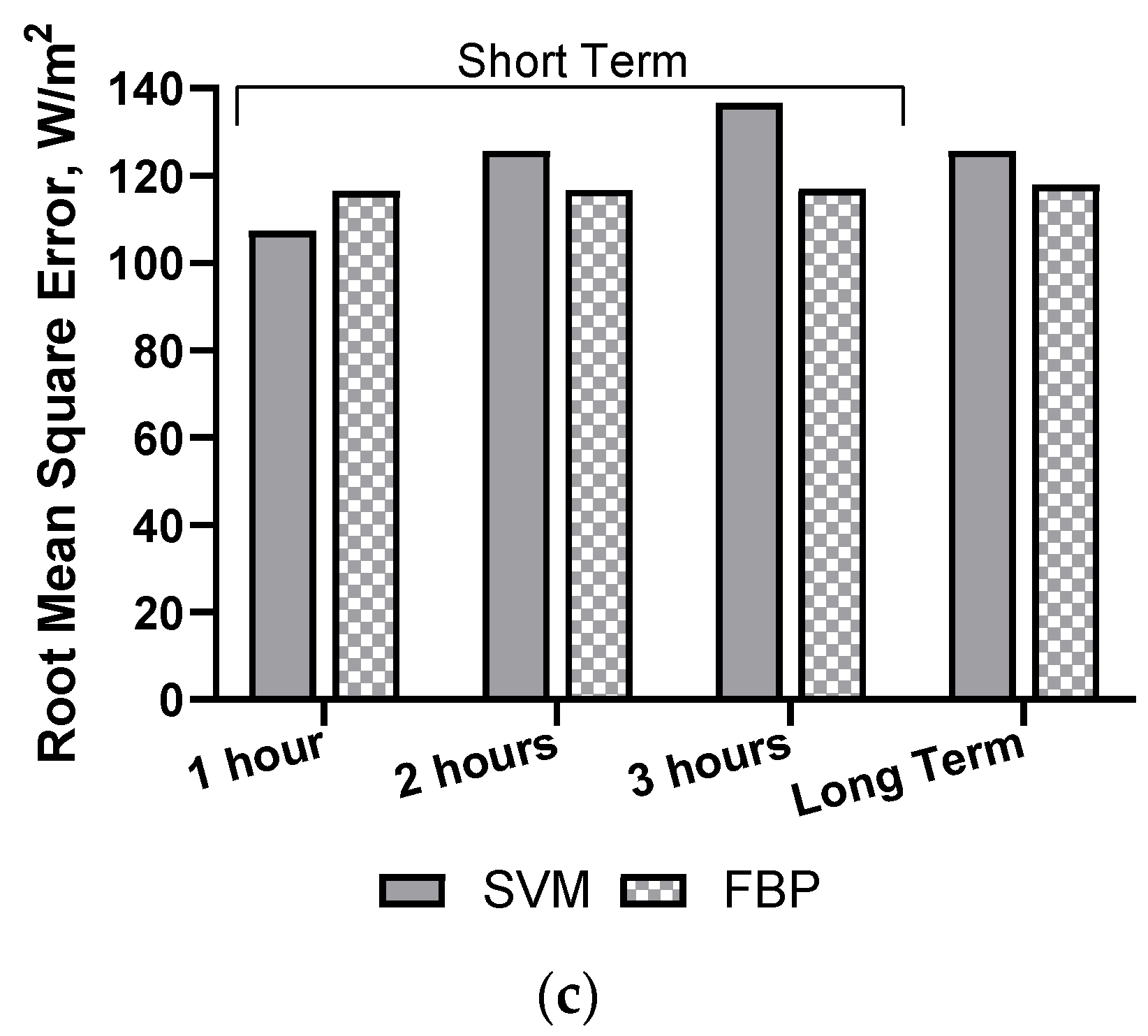
The initial model was based on historical solar radiation data and the respective algorithm. SVM outperformed FBP in the 1-hour ahead prediction in terms of R² and RMSE (

Table 4. Short-term results using data-driven and contextual optimisation.

		Data-Driven			Contextual
Algorithm	Forecast Horizon	Initial Features	Additional Features	Tuned	Negative Elimination and Night Hours	Overall Improvement
		R2
SVM	1 h	83.27%	87.45%	87.64%	87.64%	5.25%
	2 h	76.02%	82.74%	83.07%	83.07%	9.27%
	3 h	72.05%	79.56%	80.02%	80.02%	11.07%
FBP	1 h	77.84%	83.46%	83.46%	83.55%	7.34%
	2 h	77.82%	83.37%	83.37%	83.46%	7.24%
	3 h	77.82%	83.33%	83.33%	83.41%	7.18%
		MAE
SVM	1 h	73.42	55.2	46.88	46.70	36.40%
	2 h	84.71	67.5	58.86	58.86	30.51%
	3 h	89.98	74.65	65.99	65.96	26.69%
FBP	1 h	99.49	65.39	65.39	60.69	39.00%
	2 h	99.53	65.62	65.62	60.97	38.74%
	3 h	99.54	65.79	65.79	61.23	38.49%
		RMSE
SVM	1 h	124.93	108.2	107.37	107.37	14.06%
	2 h	149.55	126.90	125.68	125.68	15.96%
	3 h	161.48	138.07	136.51	136.51	15.47%
FBP	1 h	135.03	116.47	116.47	116.30	13.87%
	2 h	135.07	116.78	116.78	116.63	13.65%
	3 h	135.09	116.94	116.94	116.81	13.53%

). It also had the lowest MAE for all three horizons. For 2-hour prediction, the FBP yielded similar results in R² and MAE to SVM, while beyond this horizon, it outperformed the SVM model. This is because SVM displayed a stark decline in accuracy with the increase in prediction horizon. For the long-term forecast, FBP resulted in a better R² and RMSE, while SVM yielded a better MAE (

Table 5. Long-term results using data-driven and contextual optimisation.

	Data-Driven			Contextual
Algorithm	Initial Features	Additional Features	Tuned	Negative Elimination	Negative Elimination and Night Hours	Seasonal Adaptation	Overall Improvement
	R2
SVM	68.72%	80.32%	80.78%	80.78%	80.78%	82.56%	20.13%
FBP	77.83%	83.11%	83.11%	83.19%	83.22%	83.97%	7.89%
	MAE
SVM	72.67	54.02	55.61	55.57	55.56	56.67	22.01%
FBP	99.57	67.07	67.07	63.96	62.42	57.81	41.94%
	RMSE
SVM	160.33	127.19	125.67	125.67	125.67	119.74	25.32%
FBP	135.02	117.85	117.85	117.59	117.46	114.83	14.95%

). Adding extraterrestrial radiation to the model enhanced the performance of SVM and FBP for both the short- and long-term predictions (Table 4 and Table 5). For the short-term prediction, R² increased by ca. 7% for FBP, and between 5% (for 1 hour ahead) and 10.5%, (for 3 hours ahead) for the SVM model. MAE decreased noticeably for FBP, by ca. 34 W/m², and also, but less drastically, for the SVM model. RMSE also decreased for both algorithms. The SVM model, which included global and extraterrestrial radiation of the same hour and day, 1 and 2 years ago, yielded the best results. The R² value in the long-term model increased by 7% for FBP and 17% for SVM. Furthermore, MAE and RMSE were reduced substantially. Overall, the addition of extraterrestrial radiation resulted in considerable improvements of all models. Extraterrestrial radiation on a horizontal surface is a good indicator of potential global horizontal irradiance, stating how much solar radiation is received at the top of the atmosphere for a certain location [51].

The hyperparameters were tuned for the SVM model, using grid search cross validation. The tunable parameters were the regularisation parameter $C$, the size of the error tube $\epsilon ,$ and the width of the RBF kernel $\gamma$. The influence of $\epsilon$ and $\gamma$ were minimal, leading to improvements of less than 0.0004% in R². Therefore, it was focused on tuning the regulation parameter $C$. SVMs are generally strongly dependent on their hyperparameters [10]. However, tuning the hyperparameters for these models did not lead to significant improvements. For the short-term prediction, $C$ = 120 led to the best results. This, however, only improved R² by 0.5%, MAE by 8.6 W/m², and RMSE by 1.6 W/m². These improvements were low, compared with the addition of features. For the long-term prediction, the best $C$ was 0.5. The improvements for this were even smaller.

The results of the data-driven model can be seen in Figure 8, displaying the same trend as described for the initial model (untuned, without added features).

5.2. Contextual Optimisation Results

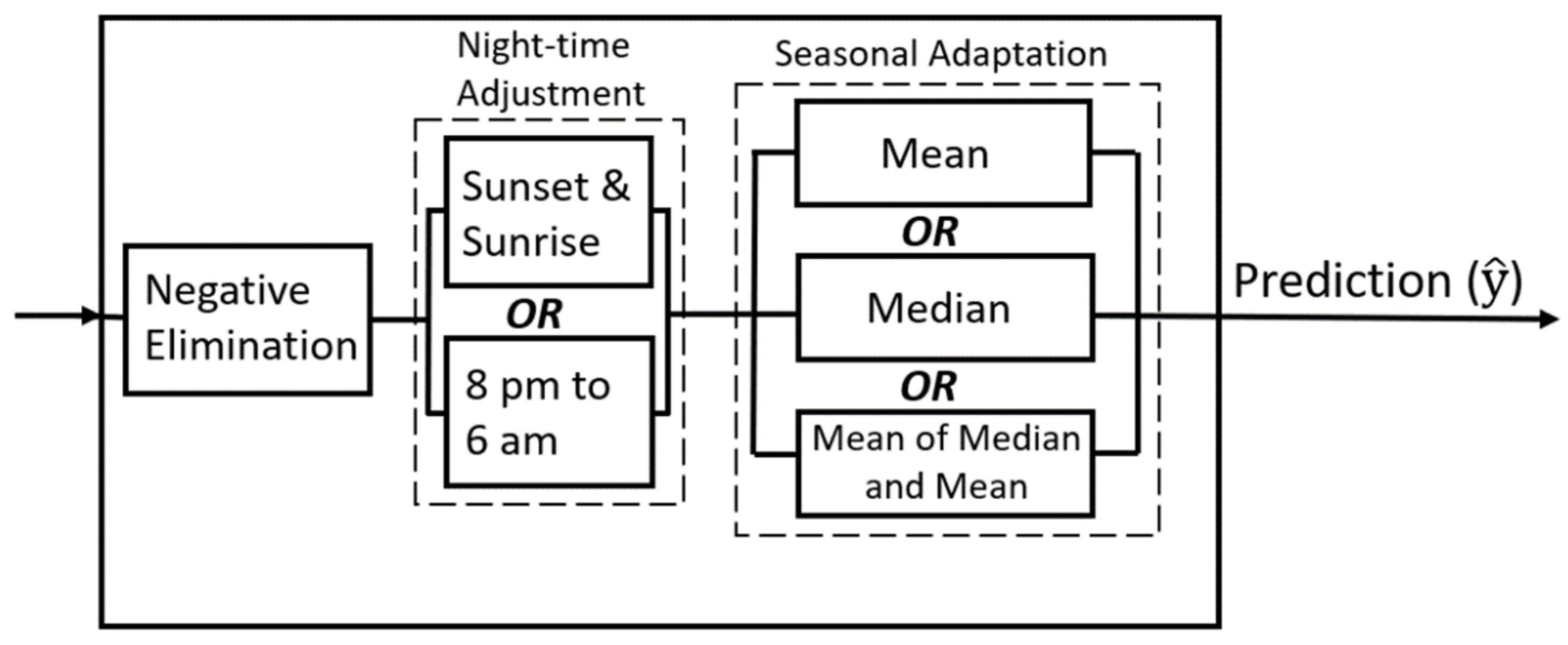
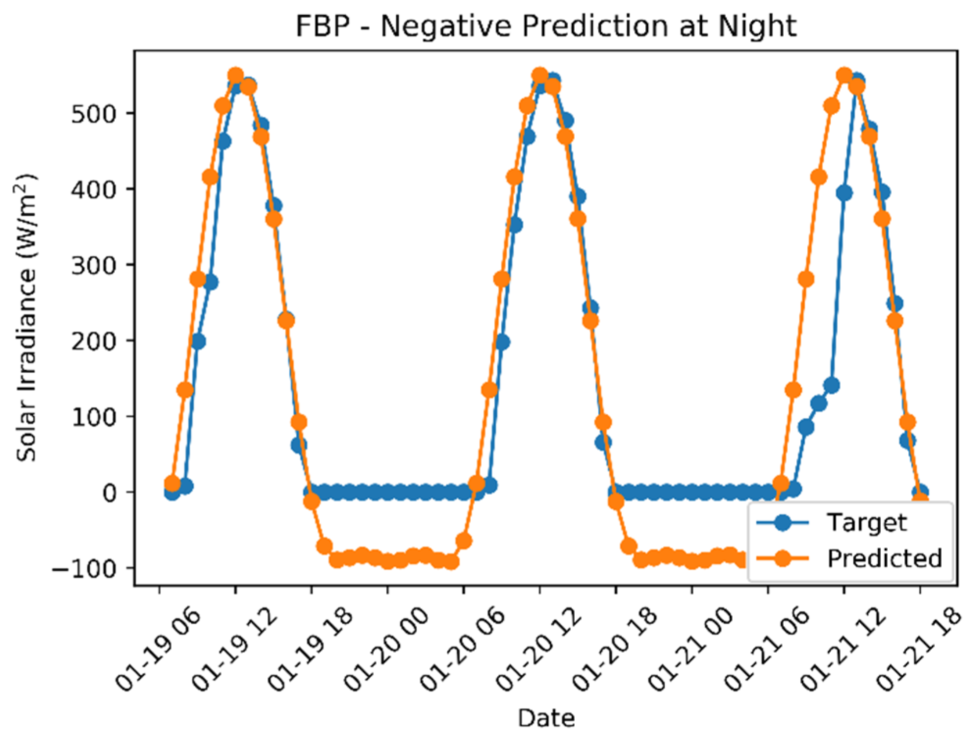
The results of further contextual optimisation are presented in this section. Setting all negative values to zero slightly improved the SVM model. It further enhanced the model, as it does not confuse the user with the prediction of impossible (negative) values. As the FBP short-term model had larger negative predictions, eliminating these led to greater improvements. The R² increased by 3% and MAE and RMSE decreased by 26 W/m² and 8 W/m², respectively. The long-term model improvements were less significant. As neither of the models predicted negative solar radiation during the day, setting all values to zero was appropriate. A model that predicted zero values at night, instead of negative values, was a closer reflection of reality.

There were some positive predictions at night. As this was not possible, sunrise and sunset adjustments were applied. Setting all values from sunset to sunrise to zero gave slightly better prediction results than defining all night hours as 8 p.m.–6 a.m. This was to be expected and true for short- and long-term predictions, in both SVM and FBP models. Including the flexible sunrise and sunset in the model allowed it to be easily applied to a location with different geographical conditions. This is particularly important in locations that are far from the equator, as sunset and sunrise vary more over the year in those places. However, it must be noted that including this adjustment into the model requires extra computational power. In locations where there is no significant variation in sunset and sunrise times during the year, this step may not be worth the marginally improved performance.

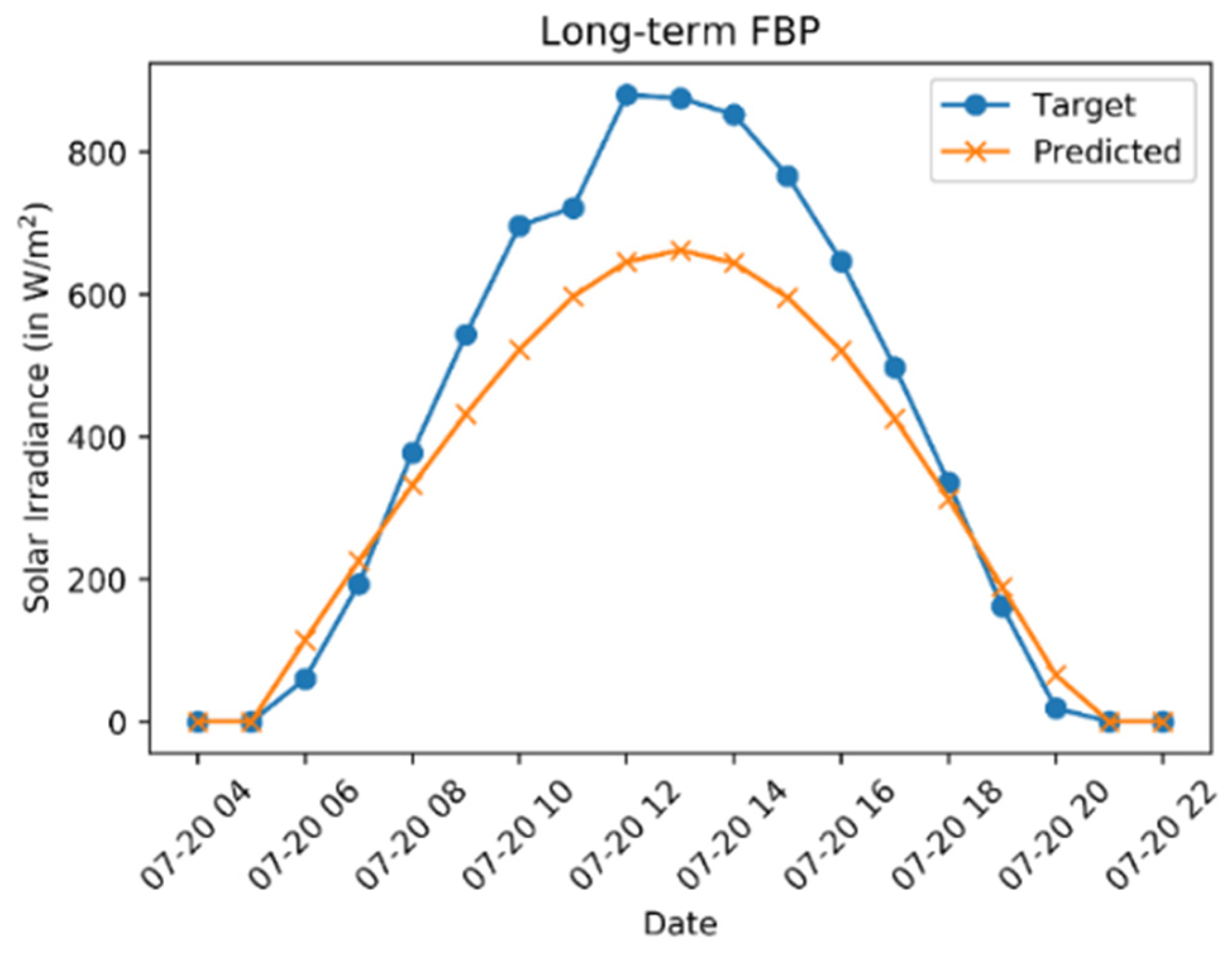
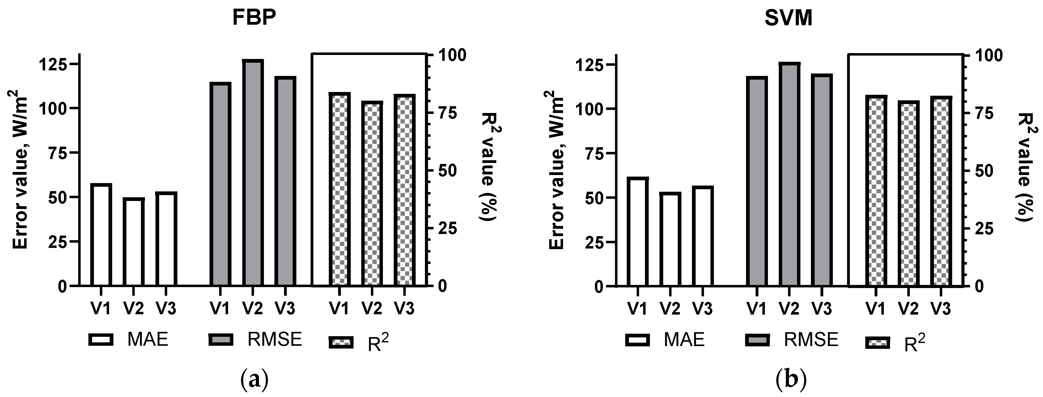
Seasonal adaptation only applied to the long-term forecast. There were three versions of this amendment, using the mean (V1), the median (V2), and the mean of the mean and median (V3). For SVM, the seasonal adaptation had a greater impact on the model with additional features. Version 1 performed best for the R² value, reducing the error by 11% and decreasing RMSE by 7 W/m², as shown in Figure 9. However, MAE increased by 6 W/m², which should be avoided. Version 2 performed better for MAE, decreasing it. However, the R² value decreased by 0.2% and RMSE increased slightly, which is also not desirable. Version 3 combines aspects of both preceding versions, offering more continuity and stable results. 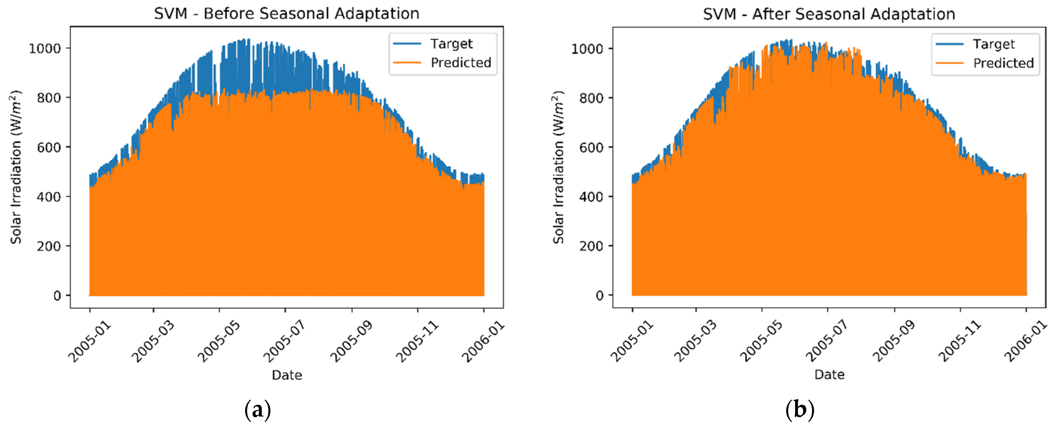The R² and RMSE values for this version were better in comparison with the previous amendment (sunrise and sunset), while MAE was very similar. Therefore, version 3 of the seasonal adaptation, using the mean of the median and mean, was chosen as the last amendment for the long-term SVM model. The improvement of applying the seasonal adaptation can clearly be observed in Figure 10.

For FBP, the improvement on the model with additional features was marginal. As version 1 (using the mean as the average) led to improvements for all metrics, it was chosen for the FBP model. Interestingly, applying the seasonal adaptation to the FBP model without the extraterrestrial radiation led to results in R², MAE, and RMSE that were only slightly different from the model with extraterrestrial radiation. The seasonal adaptation had a greater positive impact on the model without extraterrestrial radiation, as shown in

Table 6. Comparison of influence on seasonal adaptation on FBP models with different features.

	Initial Features			Initial + Additional Features
	Sunset and Sunrise	Seasonal Adaptation	Improvement	Sunset and Sunrise	Seasonal Adaptation	Improvement
R2	80.56%	83.35%	2.79%	83.22%	83.97%	0.74%
MAE	70.1	61.51	8.60	62.42	57.81	4.61
RMSE	126.4	117.01	9.42	117.46	114.83	2.62

, with the addition of correcting the daily seasonality. The impact on this model was larger because the yearly and daily seasonality were both corrected, while for the model with extraterrestrial radiation mostly daily seasonality was adjusted. Thus, using a model without extraterrestrial radiation could be considered if these data are not available.

Table 4 and Table 5 display the results of all steps of data-driven and contextual parts for short- and long-term forecasts. It is clear that the accuracy was enhanced at each step of the algorithm, starting from the initial features training to the SA. The proposed model changes improved R² of the short-term model by 5% (1 h) to 11% (3 h) for SVM and 7% for FBP. The MAE for the FBP model decreased by 39 W/m² and by ca. 25 W/m² for SVM. RMSE was also decreased by 17 to 24 W/m² for SVM and 18 W/m² for FBP. The overall R² improvement associated with model changes for the long-term forecast is 20% for SVM and 8% for FBP, as shown in Table 5. MAE decreased by 42 W/m² for FBP but only by 16 W/m² for SVM. For SVM, however, RMSE decreased by 41 W/m², whereas for FBP, it decreased by 20 W/m².

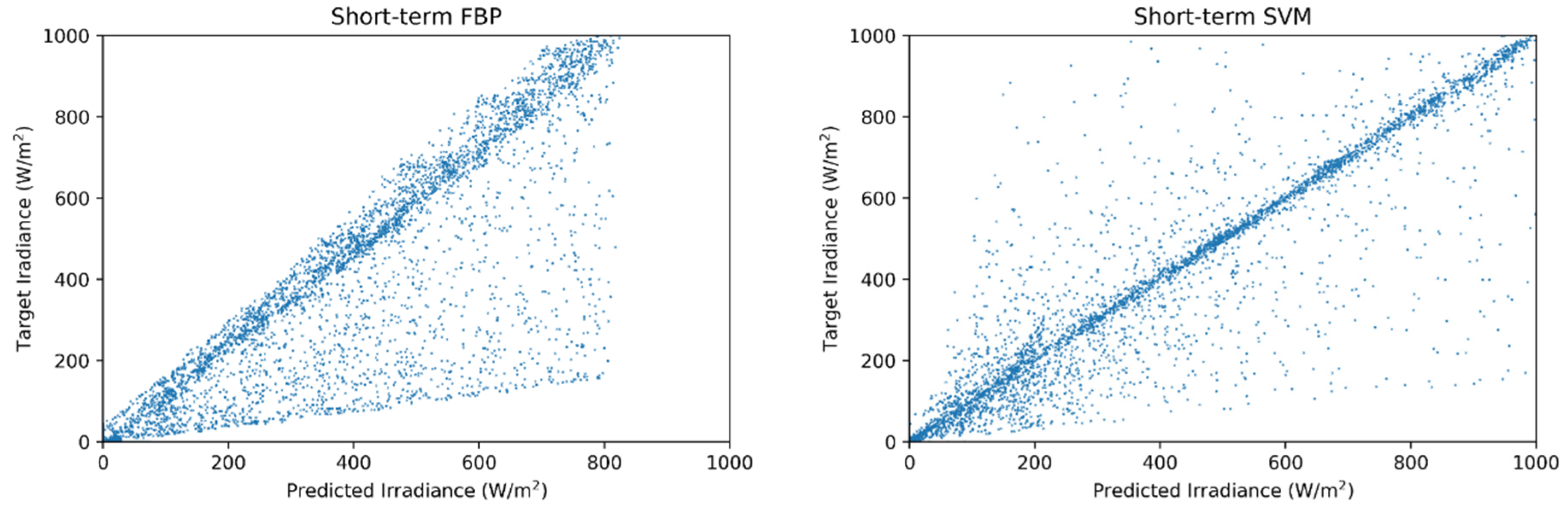
The insights of the individual model results for different horizons were taken to determine which algorithm to use for which horizon in the final DCF. For DCF, the highest accuracy for the 1- and 2-hour predictions was achieved using SVM with extraterrestrial radiation as an additional input feature, using the dynamic night-time adjustment and version 3 of the seasonal adaptation. Figure 11 shows that the 1-hour prediction SVM displayed a compact trend line with only a few normally distributed errors. For FBP, most values were on a line that was slightly too steep, indicating an overprediction for those values. However, there were also many points below the dense line, signalling underprediction. For the 3-hour and long-term predictions, the FBP using V1 of the seasonal adaptation outperformed all the other versions and algorithms. It can be concluded that the SVM model should be used for 1- and 2-hour ahead predictions, while beyond that, the FBP model should be utilised in the final DCF.

The performance of FBP suffered less from an increase in horizon than the SVM model. This is due to the underlying characteristics of the algorithm; FBP is specifically designed for time-series prediction [30]. An advantage is that the performance declines less over time. However, inputting the whole past time series into the model did not allow emphasising values that had a higher correlation and were more relevant to the particular prediction. For SVM, this could be differentiated.

5.3. DCF Performance

In this section, the DCF performance for short- and long-term forecasting is presented. To validate its performance and ensure that DCF is a generic model that can be utilised for different locations, forecasts were conducted for three cities, i.e., Denver, Boston, and Seattle.

The results for all three cities and both algorithms are presented in

Table 7. Comparison of SVM and FBP performance in all cities.

Algorithm	Horizon		Denver	Seattle	Boston
			R2
SVM	Short term	1 h	87.64%	90.62%	91.19%
		2 h	83.07%	85.80%	86.77%
		3 h	80.02%	82.32%	81.94%
	Long term	8760 h	82.56%	78.41%	75.92%
FBP	Short term	1 h	83.55%	78.35%	83.53%
		2 h	83.46%	78.32%	83.44%
		3 h	83.41%	78.32%	83.39%
	Long term	8760 h	83.97%	80.29%	78.32%
			MAE
SVM	Short term	1 h	46.70	37.40	36.15
		2 h	58.86	49.27	47.48
		3 h	65.96	58.39	57.95
	Long term	8760 h	56.67	52.90	58.67
FBP	Short term	1 h	60.69	55.94	60.96
		2 h	60.97	56.01	61.23
		3 h	61.23	56.02	61.48
	Long term	8760 h	57.81	51.04	57.86
			RMSE
SVM	Short term	1 h	107.37	75.36	77.05
		2 h	125.68	92.72	94.42
		3 h	136.51	103.48	110.29
	Long term	8760 h	119.74	106.39	116.94
FBP	Short term	1 h	116.30	103.54	116.37
		2 h	116.63	103.60	116.69
		3 h	116.81	103.60	116.87
	Long term	8760 h	114.83	98.77	110.99

. It can be seen that the SVM model performed even better on the short-term prediction in Seattle and Boston than for Denver, while the general trend remained the same as for the Denver results. For the long-term prediction, Denver displayed the best results in terms of R²; however, both MAE and RMSE were as low or lower for Boston and Seattle than for Denver. Again, the SVM model mostly outperformed FBP in the 1- and 2-hour forecasts, while the FBP model generally generated better results for 3-hour prediction and in the long term. This was observed similarly in the results and its trend validated the chosen DCF model.

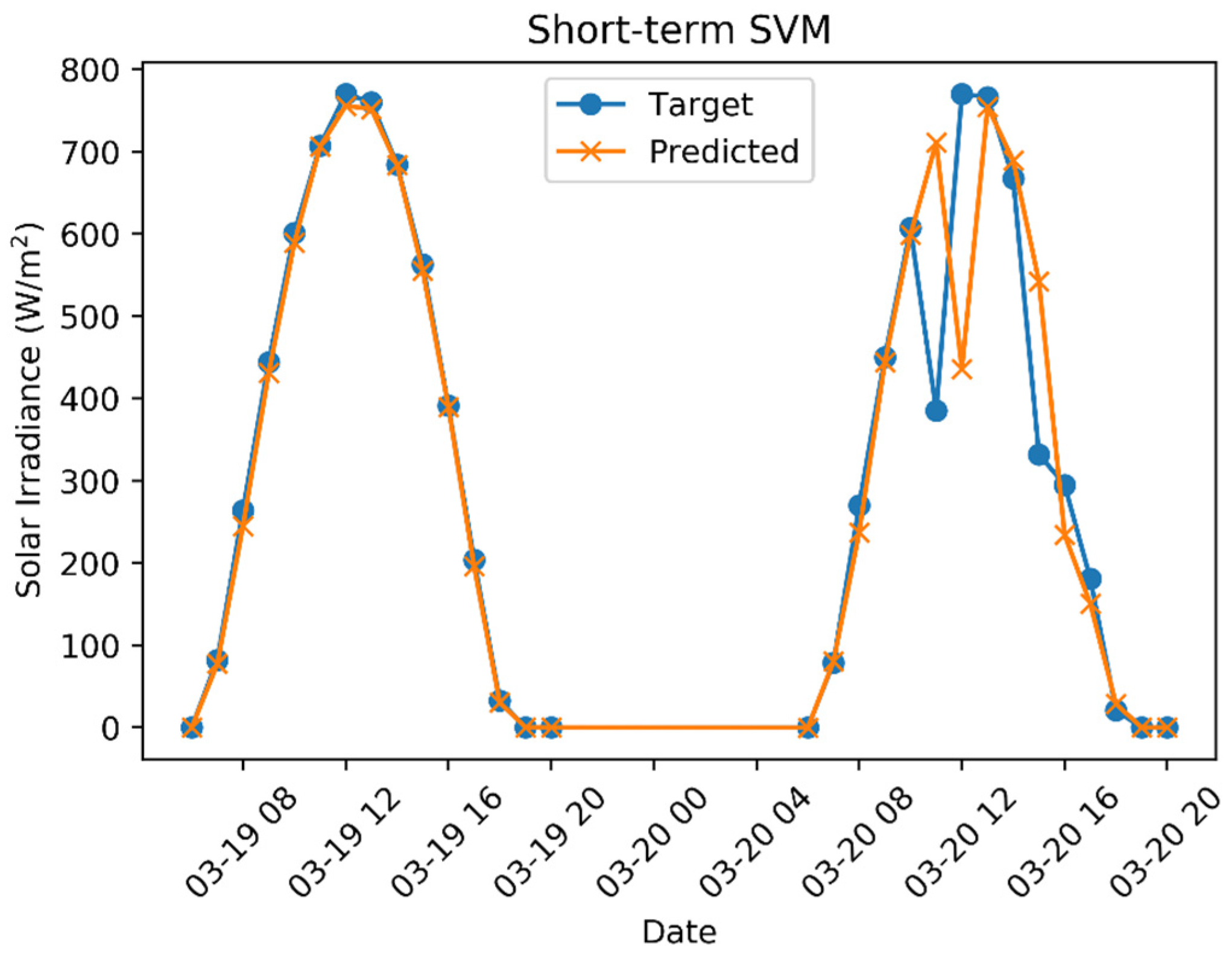
Two days of short-term predictions by the DCF algorithm are displayed in Figure 12. It shows that the model was noticeably accurate for sunny days (first day), with smooth irradiance transitions. Furthermore, it captured trends for changes in weather, as can be observed on the second day. Despite the rapid change in irradiance, the model still generated accurate predictions.

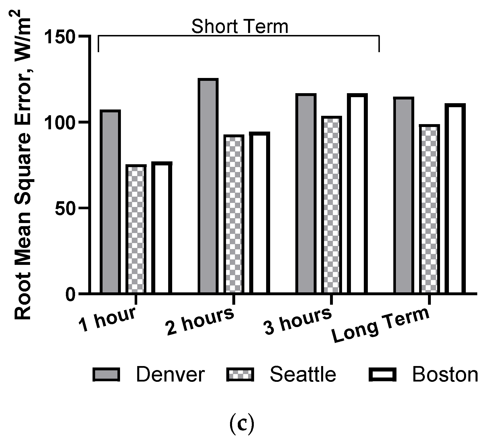
As shown in Figure 13, DCF was applicable to different locations, conserving the general pattern of performance. This validated the DCF algorithm and provided us with confidence that this model will perform well in other not-yet-tested locations. Results of around 90% (91.2%, 90.6%, and 87.6%) for the 1-hour predictions were achieved for R², while MAE ranged from 36 W/m² for Seattle to 47 W/m² for Denver and RMSE from 75 W/m² for Seattle to 107 W/m² for Denver. For the 2-hour forecast, the R² value declined by about 5%, and MAE and RMSE increased by ca. 12 and 18 W/m², respectively, for all locations. The 3-hour prediction still generated R² of 78% (Seattle) to about 83% (Denver and Boston), while MAE ranged from 56 (Seattle) to about 61 W/m² (Denver and Boston) and RMSE from 103 W/m² (Seattle) to 116 W/m² (Denver and Boston). Even the long-term prediction for one year ahead still generated good results for all cities, with high R² values and low error values, as shown in Figure 13.

6. Conclusions

This paper presented the DCF algorithm, a forecasting algorithm that accurately predicts solar irradiance. Unlike other state-of-the-art models, the forecast accuracy was validated for short- and long-term predictions in three cities. The DCF algorithm had two main parts. Initially, it utilised the most accurate data-driven (ML) algorithms and then optimised their performance using contextual information. SVM and FBP were used as the data-driven models. SVM has been used for solar forecasting for over a decade. FBP, in contrast, is a novel algorithm that has rarely been used in the field of solar prediction. Nevertheless, its design characteristics seemed inherently promising for solar prediction.

Firstly, a basic model was constructed for both algorithms with only hourly solar irradiance as input. The data were taken from the National Solar Radiation Database (NSRDB). Adding extraterrestrial radiation led to the largest improvement in R², MAE, and RMSE, for both SVM and FBP models. For the SVM model, the regularisation parameter $C$ was tuned using grid search cross validation. This did not have a significant impact on the performance of the model. After training the model with the additional input features and the tuned hyperparameters, solar irradiance was predicted. The prediction was subject to several adjustments. All negative values and all values between sunset and sunrise were set to zero. This had a greater impact on FBP than on SVM, as FBP would generate larger non-zero predictions at night. Furthermore, a seasonal adaptation was applied. This increased or decreased every hour of the day for each month if it was above or below the average of the last years. It led to a significant improvement, as shown in Table 6.

For the 1-hour short-term prediction, the final SVM model outperformed FBP and, thus, was utilised for the DCF algorithm. As shown in Table 7, it achieved an R² value of 87.6% for Denver, 90.6% for Seattle, and 91.2% for Boston. An MAE value of 36 W/m² was attained for Boston and similar values for Seattle and Denver. RMSE varied from 75 W/m² (Seattle) and 77 W/m² (Boston) to 107 W/m² (Denver). For the 2-hour prediction, SVM mostly outperformed FBP. On occasions in which this was not the case, the results were very similar. However, the SVM model displayed a strong decrease in forecasting accuracy with the increase in the forecast horizon. Therefore, for the 3-hour prediction, the FBP model yielded better results and thus was used beyond the 3-hour forecast in the DCF algorithm. The FBP performance only decreased very slightly over time, compared to the SVM. The reason for its sustained performance is its specific design for time-series predictions. The FBP model performed better for the long-term forecast than the SVM model. This was true for all cities and thus validated the use of the suggested model.

7. Future Research

Improvements may arise from analysing and adding further meteorological input features. This could, for example, be a measure of cloud cover or temperature. Care must be taken that no features are included that either worsen the prediction or have no positive impact while making the model more complicated. Adding features could be advantageous for the SVM model, as for SVM, any features can be added, while for FBP, only features that are known in the future can be added.

The SVM model might be improved by further analysing the correlation of the irradiance with past values. This could reveal correlations with hours that have not yet been used as input features. Adding these would be a promising path to further enhance the model. This also suggests another set of experiments that could be executed to examine the mid-term horizon for both SVM and FBP models. FBP might be better at mid-term forecasts, e.g., 3 months. However, this has not been experimentally investigated. A correlation analysis would be of great use for a mid-term SVM model and would therefore lend itself to being carried out in parallel with a comparative analysis of mid-term SVM and FBP models.

The long-term FBP model showed that applying the seasonal adaptation to Denver nearly made the extraterrestrial radiation redundant. Both models, with and without extraterrestrial radiation, displayed similar results. This could be useful for datasets that do not possess measurements of extraterrestrial radiation. Therefore, the benefits of only seasonal adaptation instead of adding extraterrestrial radiation to the model should be explored further.

References

1. Thompson, L.G. Climate change: The evidence and our options. Behav. Anal. 2010, 33, 153–170. [Google Scholar] [CrossRef]
2. EPA-United States Environmental Protection Agency. Sources of Greenhouse Gas Emissions. Available online: https://www.epa.gov/ghgemissions/sources-greenhouse-gas-emissions (accessed on 20 October 2021).
3. Newell, P.; Simms, A. How Did We Do That? Histories and Political Economies of Rapid and Just Transitions. New Political Econ. 2020, 26, 907–922. [Google Scholar] [CrossRef]
4. Huybrechts, B. Social Enterprise, Social Innovation and Alternative Economies: Insights from Fair Trade and Renewable Energy. In Alternative Economies and Spaces: New Perspectives for a Sustainable Economy; Transcript Verlag: Bielefeld, Germany, 2013; pp. 113–130. [Google Scholar]
5. Jia, Y.; Lyu, X.; Lai, C.S.; Xu, Z.; Chen, M. A retroactive approach to microgrid real-time scheduling in quest of perfect dispatch solution. J. Mod. Power Syst. Clean Energy 2019, 7, 1608–1618. [Google Scholar] [CrossRef] [Green Version]
6. Perera, K.S.; Aung, Z.; Woon, W.L. Machine Learning Techniques for Supporting Renewable Energy Generation and Integration: A Survey. In International Workshop on Data Analytics for Renewable Energy Integration; Springer: Cham, Switzerland, 2014; pp. 81–96. [Google Scholar] [CrossRef]
7. Fouilloy, A.; Voyant, C.; Notton, G.; Motte, F.; Paoli, C. Solar irradiation prediction with machine learning: Forecasting. Energy 2018, 165, 620–629. [Google Scholar] [CrossRef]
8. IEA. Fossil Fuel Energy Consumption; International Energy Agency: Paris, France, 2020. [Google Scholar]
9. International Renewable Energy Agency. IRENA—Download Data. 2020. Available online: https://www.irena.org/Statistics/Download-Data (accessed on 12 January 2021).
10. Van der Wiel, K.; Bloomfield, H.C.; Lee, R.W.; Stoop, L.P.; Blackport, R.; Screen, J.A.; Selten, F.M. The influence of weather regimes on European renewable energy production and demand. Environ. Res. Lett. 2019, 14, 94010. [Google Scholar] [CrossRef]
11. Staffell, I.; Pfenninger, S. The increasing impact of weather on electricity supply and demand. Energy 2017, 145, 65–78. [Google Scholar] [CrossRef]
12. Sobri, S.; Koohi-Kamali, S.; Rahim, N.A. Solar photovoltaic generation forecasting methods: A review. Energy Convers. Manag. 2018, 156, 459–497. [Google Scholar] [CrossRef]
13. Arraez-Cancelliere, O.A.; Muñoz-Galeano, N.; López-Lezama, J.M. Computing the Global Irradiation over the Plane of Photovoltaic Arrays: A Step-by-Step Methodology. In Renewable Energy—Technologies and Applications; Taner, T., Tiwari, A., Ustun, T.S., Eds.; IntechOpen: London, UK, 2020. [Google Scholar]
14. Wang, H.; Liu, Y.; Zhou, B.; Li, C.; Cao, G.; Voropai, N.; Barakhtenko, E. Taxonomy research of artificial intelligence for deterministic solar power forecasting. Energy Convers. Manag. 2020, 214, 112909. [Google Scholar] [CrossRef]
15. Net Zero Strategy: Build Back Greener October 2021. Available online: https://assets.publishing.service.gov.uk/government/uploads/system/uploads/attachment_data/file/1033990/net-zero-strategy-beis.pdf (accessed on 20 October 2021).
16. Kahwash, F.; Barakat, B.; Taha, A.; Abbasi, Q.H.; Imran, M.A. Optimising Electrical Power Supply Sustainability Using a Grid-Connected Hybrid Renewable Energy System—An NHS Hospital Case Study. Energies 2021, 14, 7084. [Google Scholar] [CrossRef]
17. Sanjari, M.J.; Gooi, H.B. Probabilistic Forecast of PV Power Generation Based on Higher Order Markov Chain. IEEE Trans. Power Syst. 2016, 32, 2942–2952. [Google Scholar] [CrossRef]
18. Kavasseri, R.G.; Seetharaman, K. Day-ahead wind speed forecasting using f-ARIMA models. Renew. Energy 2009, 34, 1388–1393. [Google Scholar] [CrossRef]
19. Guariso, G.; Nunnari, G.; Sangiorgio, M. Multi-Step Solar Irradiance Forecasting and Domain Adaptation of Deep Neural Networks. Energies 2020, 13, 3987. [Google Scholar] [CrossRef]
20. Jiang, H.; Dong, Y. Forecast of hourly global horizontal irradiance based on structured kernel support vector machine: A case study of Tibet area in China. Energy Convers. Manag. 2017, 142, 307–321. [Google Scholar] [CrossRef]
21. Zendehboudi, A.; Baseer, M.; Saidur, R. Application of support vector machine models for forecasting solar. J. Clean. Prod. 2018, 199, 272–285. [Google Scholar] [CrossRef]
22. Bae, K.Y.; Jang, H.S.; Sung, D.K. Hourly solar irradiance prediction based on support vector machine and its error analysis. IEEE Trans. Power Syst. 2016, 32, 935–945. [Google Scholar] [CrossRef]
23. Mueller, K.R.; Smola, A.J.; Raetsch, G.; Schoelkopf, B.; Kohlmorgen, J. Using Support Vector Machines for Time Series Prediction; GMD FIRST: Berlin, Germany, 2000. [Google Scholar]
24. Fentis, A.; Bahatti, L.; Mestari, M.; Chouri, B. Short-term solar power forecasting using Support Vector Regression and feed-forward NN. In Proceedings of the 2017 15th IEEE International New Circuits and Systems Conference (NEWCAS), Strasbourg, France, 25–28 June 2017; pp. 405–408. [Google Scholar] [CrossRef]
25. Ramedani, Z.; Omid, M.; Keyhani, A.; Shamshirband, S.; Khoshnevisan, B. Potential of radial basis function based support vector regression for global solar radiation prediction. Renew. Sustain. Energy Rev. 2014, 39, 1005–1011. [Google Scholar] [CrossRef]
26. Meenal, R.; Selvakumar, A.I. Assessment of SVM, empirical and ANN based solar radiation prediction models with most influencing input parameters. Renew. Energy 2018, 121, 324–343. [Google Scholar] [CrossRef]
27. Boyd, S. Convex Optimization; Cambridge University Press: Cambridge, UK, 2004. [Google Scholar]
28. Zeng, J.; Qiao, W. Short-term solar power prediction using a support vector machine. Renew. Energy 2013, 52, 118–127. [Google Scholar] [CrossRef]
29. VanDeventer, W.; Jamei, E.; Thirunavukkarasu, G.S.; Seyedmahmoudian, M.; Soon, T.K.; Horan, B.; Mekhilef, S.; Stojcevski, A. Short-term PV power forecasting using hybrid GASVM technique. Renew. Energy 2019, 140, 367–379. [Google Scholar] [CrossRef]
30. Taylor, S.J.; Letham, B. Forecasting at Scale. Am. Stat. 2017, 72, 37–45. [Google Scholar] [CrossRef]
31. Lim, J.Y.; Safder, U.; How, B.S.; Ifaei, P.; Yoo, C.K. Nationwide sustainable renewable energy and Power-to-X deployment planning in South Korea assisted with forecasting model. Appl. Energy 2020, 283, 116302. [Google Scholar] [CrossRef]
32. Shawon, M.H.; Akter, S.; Islam, K.; Ahmed, S.; Rahman, M. Forecasting PV panel output using prophet time. In Proceedings of the 2020 IEEE REGION 10 CONFERENCE (TENCON), Osaka, Japan, 16–19 November 2020. [Google Scholar]
33. Žunić, E.; Korjenić, K.; Hodžić, K.; Dženana, Đ. Application of Facebook’s Prophet Algorithm for Successful Sales Forecasting Based on Real-world Data. Int. J. Comput. Sci. Inf. Technol. 2020, 12, 23–36. [Google Scholar] [CrossRef]
34. National Renewable Energy Laboratory. National Solar Radiation Database 1991–2005 Update: User’s Manual; National Renewable Energy Laboratory: Golden, CA, USA, 2007. [Google Scholar]
35. Kalogirou, S. Solar Energy Engineering: Processes and Systems; Academic Press: Cambridge, MA, USA, 2013. [Google Scholar]
36. Malvoni, M.; De Giorgi, M.G.; Congedo, P.M. Forecasting of PV Power Generation using weather input data-preprocessing techniques. Energy Procedia 2017, 126, 651–658. [Google Scholar] [CrossRef]
37. Voyant, C.; Notton, G.; Kalogirou, S.; Nivet, M.-L.; Paoli, C.; Motte, F.; Fouilloy, A. Machine learning methods for solar radiation forecasting: A review. Renew. Energy 2017, 105, 569–582. [Google Scholar] [CrossRef]
38. Sreekumar, S.; Bhakar, R. Solar Power Prediction Models: Classification Based on Time Horizon, Input, Output and Ap-plication. In Proceedings of the 2018 International Conference on Inventive Research in Computing Applications (ICIRCA), Coimbatore, India, 3 January 2019. [Google Scholar]
39. Martín-Pomares, L.; Martínez, D.; Polo, J.; Perez-Astudillo, D.; Bachoura, D. Analysis of the long-term solar potential for electricity generation in Qatar. Renew. Sustain. Energy Rev. 2017, 73, 1231–1246. [Google Scholar] [CrossRef]
40. Olatomiwa, L.; Mekhilef, S.; Shamshirband, S.; Mohammadi, K.; Petković, D.; Sudheer, C. A support vector machine–firefly algorithm-based model for global solar radiation prediction. Sol. Energy 2015, 115, 632–644. [Google Scholar] [CrossRef]
41. Quej, V.H.; Almorox, J.; Arnaldo, J.A.; Saito, L. ANFIS, SVM and ANN soft-computing techniques to estimate daily global solar radiation in a warm sub-humid environment. J. Atmos. Sol.-Terr. Phys. 2017, 155, 62–70. [Google Scholar] [CrossRef] [Green Version]
42. Wolff, B. Statistical Learning for Short-Term Photovoltaic Power Predictions. In Computational Sustainability; Springer: Berlin/Heidelberg, Germany, 2016. [Google Scholar]
43. Long, H.; Zhang, Z.; Su, Y. Analysis of daily solar power prediction with data-driven approaches. Appl. Energy 2014, 126, 29–37. [Google Scholar] [CrossRef]
44. Van Rossum, G. Python Tutorial; Centrum voor Wiskunde en Informatica (CWI): Amsterdam, The Netherlands, 1995. [Google Scholar]
45. Pedregosa, F.; Varoquaux, G.; Gramfort, A.; Michel, V.; Thirion, B.; Grisel, O.; Blondel, M.; Prettenhofer, P.; Weiss, R.; Dubourg, V.; et al. Scikit-learn: Machine Learning in Python. J. Mach. Learn. Res. 2011, 12, 2825–2830. [Google Scholar]
46. Guyon, I.; Elisseeff, A. An Introduction to Variable and Feature Selection. J. Mach. Learn. Res. 2003, 3, 1157–1182. [Google Scholar]
47. Abuella, M.; Chowdhury, B. Solar Power Forecasting Using Support Vector Regression. In Proceedings of the American Society for Engineering Management International Annual Conference Charlotte, NC, USA, 26–29 October 2016. [Google Scholar]
48. Mantovani, R.G.; Rossi, A.L.D.; Vanschoren, J.; Bischl, B.; de Carvalho, A.C.P.L.F. Effectiveness of Random Search in SVM hyper-parameter tuning. In Proceedings of the 2015 International Joint Conference on Neural Networks (IJCNN), Killarney, Ireland, 12–17 July 2015; pp. 1–8. [Google Scholar] [CrossRef] [Green Version]
49. Dong, Z.; Yang, D.; Reindl, T.; Walsh, W.M. A novel hybrid approach based on self-organizing maps, support vector regression and particle swarm optimization to forecast solar irradiance. Energy 2015, 82, 570–577. [Google Scholar] [CrossRef]
50. Piri, J.; Shamshirband, S.; Petković, D.; Tong, C.W.; Rehman, M.H.U. Prediction of the solar radiation on the Earth using support vector regression technique. Infrared Phys. Technol. 2015, 68, 179–185. [Google Scholar] [CrossRef]
51. Maleki, S.A.M.; Hizam, H.; Gomes, C. Estimation of Hourly, Daily and Monthly GlobalSolar Radiation on Inclined Surfaces: Models Re-Visited. Energies 2017, 10, 134. [Google Scholar] [CrossRef] [Green Version]
Figure 1. Increase in solar power generation worldwide [9].
Applsci 12 00134 g001
Figure 2. The 1D and 2D representations of average irradiance in Boston and Denver [34]. (a) 1D representation of average irradiance in Boston (b) 1D representation of average irradiance in Denver (c) 2D representation of average irradiance in Boston (d) 2D representation of average irradiance in Denver.
Applsci 12 00134 g002
Figure 3. Block diagram of DCF, showing its two main parts: data-driven model and contextual optimisation.
Applsci 12 00134 g003
Figure 4. Contextual optimisation block diagram showing the three main steps.
Applsci 12 00134 g004
Figure 5. Three days of long-term FBP prediction displaying negative values at night.
Applsci 12 00134 g005
Figure 6. FBP, displaying overprediction in morning and evening and underprediction at noon.
Applsci 12 00134 g006
Figure 7. Example of working principle: grouping the average into one value per hour per month.
Applsci 12 00134 g007
Figure 8. Error metrics comparing SVM and FBP for data-driven short- and long-term forecasts in Denver. (a) Coefficient of determination (R2) (b) Mean absolute error (c) Root-mean-square error.
Applsci 12 00134 g008aApplsci 12 00134 g008b
Figure 9. Comparison of (a) FBP and (b) SVM of seasonal adaptation versions.
Applsci 12 00134 g009
Figure 10. SVM (a) before and (b) after seasonal adaptation.
Applsci 12 00134 g010
Figure 11. Short-term FBP, SVM predicted, and target values: 1 h ahead.
Applsci 12 00134 g011
Figure 12. Two days of 1-hour ahead SVM prediction in Boston.
Applsci 12 00134 g012
Figure 13. DCF accuracy, evaluated in three cities using all evaluation metrics. (a) Coefficient of determination (R2) (b) Mean absolute error (c) Root-mean-squared error.
Applsci 12 00134 g013aApplsci 12 00134 g013b