Evaluation of Artificial Intelligence-Based Models for Classifying Defective Photovoltaic Cells

Abstract

Solar Photovoltaic (PV) energy has experienced an important growth and prospect during the last decade due to the constant development of the technology and its high reliability, together with a drastic reduction in costs. This fact has favored both its large-scale implementation and small-scale Distributed Generation (DG). PV systems integrated into local distribution systems are considered to be one of the keys to a sustainable future built environment in Smart Cities (SC). Advanced Operation and Maintenance (O&M) of solar PV plants is necessary. Powerful and accurate data are usually obtained on-site by means of current-voltage (I-V) curves or electroluminescence (EL) images, with new equipment and methodologies recently proposed. In this work, authors present a comparison between five AI-based models to classify PV solar cells according to their state, using EL images at the PV solar cell level, while the cell I-V curves are used in the training phase to be able to classify the cells based on its production efficiency. This automatic classification of defective cells enormously facilitates the identification of defects for PV plant operators, decreasing the human labor and optimizing the defect location. In addition, this work presents a methodology for the selection of important variables for the training of a defective cell classifier.

1. Introduction

During the last decade, worldwide installation of renewable generation plants has considerably increased. Among renewables, photovoltaic (PV) solar plants have been the most interesting in recent years, and it seems that they will be the most installed in the following years [1,2]. During 2019, the last analyzed year in the Global Status Report [3], 201 GW of renewable power capacity were installed in the World; 115 GW of Solar PV capacity, corresponding to more than 57% of total renewable additions. The solar PV cumulative installed capacity was raised to 633.7 GW by the end of 2019.

The reason for the spectacular growth and prospect of this energy source lies in the constant development of the technology and its high reliability. This has made possible a drastic reduction in costs, which has favored both its large-scale implementation and small-scale Distributed Generation (DG). Many countries have already begun to review their climate and energy policies. Innovation in sustainable energy supply is, thus, crucial for providing reliable and clean energy sources and improving the quality of life on this planet. To achieve this goal, the idea of smart energy buildings or energy-neutral buildings has been launched. The main objective of an energy regulation of a building is to maintain internal thermal comfort, as well as minimizing energy consumption [4]. PV systems and electric vehicles (EVs) integrated into local distribution systems are considered to be two of the keys to a sustainable future built environment in Smart Cities (SC) [5]. The term “smart energy city” has arisen in parallel with these developments, notably since at least the turn of the 2010s in connection with the energy-relevant components of smart cities [6]. In this scenario, ensuring energy production is a key factor in warranting plant profitability, and this has forced the design of increasingly intelligent and advanced operation and maintenance (O&M) strategies.

The O&M of PV solar plants is critical for industry players. The development of new equipment and methodologies for its application in PV solar plants is necessary, and in this sense, research and industry in this area are rapidly evolving [7]. Some researchers have worked with real data from PV solar plants, and they have obtained important results showing defects in them [8]. The PV inverter is a critical element in PV solar plants, but so is the PV solar module. A PV solar module is made up of PV solar cells, and these cells can have different problems or defects, as shown in [9]. Although the knowledge at the PV solar cell level is interesting for operators and maintainers of PV solar plants, the measurements should be taken in the PV solar module.

The detection of faults in PV solar modules is subject to obtaining field data, as currently, monitoring does not reach the module level in PV plants. Powerful and accurate data can be obtained by current-voltage (I-V) curves, both from the PV solar cell (when the cell contacts can be accessed) or at the PV solar module level [9,10]. Nowadays, I-V tracers present some drawbacks, such as being only for the string level, working offline, or being expensive. However, advanced instruments recently developed allow automating the online module I-V curves acquisition without requiring the PV plant to be shut down [11]. Additionally, it is also possible to perform online dark I-V curves of modules in PV plants without the need to disconnect them from the string. For this, a combination of electronic boards in the PV modules and a bidirectional inverter is required, as presented in [12].

Another way to obtain field data is by taking images. Classically, thermographic imaging (IRT) has been used for early detection of hot spots [13], and in recent years this IRT method has been carried out using drone flight [14,15]. One of the most promising maintenance techniques is the study of electroluminescence (EL) images as a complement of IRT analysis. However, its high cost has prevented its use regularly up to date. The authors in [16] proposed a maintenance methodology to perform on-site EL inspections as efficiently as possible using a bidirectional inverter.

All these inspection techniques make it possible to locate and identify the defects present in PV modules. However, nowadays, solar plants are becoming larger, and the manual treatment of all the data obtained through the previous techniques presented can be a very expensive and time-consuming task. Artificial Intelligence (AI) is already being applied in PV solar plants. AI application has long focused on energy production forecasting issues. The authors in [17] developed a solution that provides electricity production based on historical and current available solar radiation data in real-time. Other authors have presented a taxonomy study, showing a process to divide and classify the different forecasting methods, and the authors also presented the trends in AI applied to generation forecasting in solar PV plants [18]. The use of artificial neural networks (ANN) has been successful in the last decade; some authors use ANNs together with climatic variables to forecast generation in PV solar plants [19], while others use Support Vector Machine (SVM) together with an optimization of the internal parameters of the model [20].

ANNs have also been used for other tasks, such as for the detection of problems in energy production, as is the case in [21], where the authors use radial basis function (RBF) to detect this type of failure in production. A similar goal is sought in [22], where an SVM-based model was employed for describing a failure diagnosis method that uses the linear relationship between the solar radiation and the power generation graphs. This research studies the following failure types: inverter failures, communication errors, sensor failures, junction box errors, and junction box fires. The model classifies string and inverter failures. However, in actual PV plants, each inverter can cover thousands of modules, and therefore important failure information can be lost during classification.

Therefore, it is possible to affirm that the use of AI is common in PV solar plants. Research has studied its application in energy production forecasting issues or for the detection of problems in energy production. However, it has been highlighted how the detection of defects using inverter-level information can be imprecise. In this work, the authors present a comparison between five AI-based models to classify PV solar cells according to their state based on EL images. The five well-known models used for classification have been: k-nearest neighbors (KNN), SVM, Random Forests (RF), Multilayer Perceptron (MLP), and Convolutional Neural Networks (CNNs). This automatic classification of defective cells enormously facilitates the identification of defects in a precise way for PV plant operators, decreasing the human labor and optimizing the defect location. For this, the authors used an ad-hoc PV solar module manufactured in a special way since PV solar cells have their back contacts accessible, allowing their total characterization [9]. With this manufactured module, it was possible to obtain each cell I-V curve, in addition to EL images, so it was feasible to label each cell (group 1: good, group 2: fair, and group 3: bad) based on its production efficiency. This allowed an accurate classification for model training. The study presents a novel method for the labeling of cells based on their production efficiency, and this was possible due to the customized PV solar module, which clearly differentiates this research. The classifications discussed in this document are an extension of the previous work “Photovoltaic cell defect classifier: a model comparison” presented at the Smart Cities—III Iberoamerican Congress on Smart Cities (ICSC-CITIES 2020) [23]. The document is structured as follows: Section 2 presents the materials and methodology used, Section 3 shows the results, and Section 4 contains conclusions and future work proposals.

2. Materials and Methods

This section is intended to explain the materials used, as well as the methodology followed to validate the classifier.

2.1. Materials

A 60-cells polycrystalline module composed of cells with and without defects was used. The front and back views of the module are presented in Figure 1a,b respectively. The module was ad-hoc manufactured with all cells accessible from the backside of the module. Regarding the cell labeling, numbers from 0 to 59 have been used to identify the cell, as detailed in Figure 2. Additionally, the four corner cells have been labeled both in Figure 1a,b to facilitate understanding.

The first string (first and second columns in the back view) contains manufacturing defects, the central string (third and fourth columns) contains soldering faults, while the third string (fifth and sixth columns in the back view) contains breaking deficiencies. The low-efficiency defects (cells 1 and 4) and medium efficiency cells (cells 14 and 17) were due to manufacturing problems, with an efficiency of 9% and 16.4% approximately, but they did correspond with breaking or short-circuited cells. Short-circuit cell (cell 6) has been generated by extending the cell connection tabs beyond the ordinary placement, short-circuiting the cell. In order to simulate the bad soldering defects, buses from the back of some cells were left without soldering, either one bus (cell 22) or two buses (cell 34). Three buses have not been left without soldering in any case as it would have meant that this cell would not be series connected as the rest. In cell 38, all tabs were lose (without soldering), although they made contact allowing module production. The cell with only 1 cm welded (cell 27) was used to simulate bad soldering, in which only 1 cm of the bus was welded instead of the typical 15 cm being welded. The third-string contains some cracked cells without cell area decrease (cell 50 and 51), with cell area decrease (cell 41, 42, 55, and 57) or a combination of both in the same cell (cell 45). When a piece of broken cell was placed on top of another cell (cells 49, 58, and 59), it generates partial shading, simulating the important aspect of permanent bird droppings. These types of defects were analyzed as they ordinarily appear in commercial modules in operation, either during manufacturing, transport, or operation. However, commercial modules are not accessible at the cell level. That is why an ad hoc module was manufactured for defect characterization.

The nominal characteristics of a standard module of this type are: nominal power (P) 250 W, efficiency 15.35%, maximum power point current (Impp) 8.45 A, maximum power point voltage (Vmpp) 29.53 V, short circuit current (Isc) 8.91 A and open-circuit voltage (Voc) 37.6 V. Having 60 cells in series, the nominal values of a healthy cell were considered: nominal power 4.17 W, Impp 8.45 A, Vmpp 0.49 V, Isc 8.91 A, and Voc 0.63 V.

I-V curve measurement (at the cell level) and EL images were carried out at the CIEMAT’s facilities (Madrid, Spain). In summary, the facilities used were the following:

• The indoor measurements have been performed in the commercial system Pasan SunSim 3 CM, which consisted of a light pulse solar simulator class AAA according to IEC 60904-9 standard, which can perform I-V curve measurements at Standard Test conditions;
• The EL and indoor IRT tests were simultaneously performed with the EL in this chamber. The module was fed with a Delta power supply SM 70-22. A Fluke 189 multimeter connected to module terminals allowing it to register the exact module voltage. EL and IR images were captured with a PCO 1300 and a FLIR SC 640 camera, respectively.

In this way, the information of the EL image and I-V curve of each PV solar cell was obtained. In the following Figure 2, an EL image of the measurement module and the numbering of the cells is shown.

This information could serve to validate the different models. In the training phase, the cells used were labeled according to their potency (measured through the I-V curve) and with the following criteria:

• Group 1: Power ≥ 95%;
• Group 2: 80% ≤ Power < 95%;
• Group 3: Power < 80%.

According to the measured I-V curves, the classification of the cells in the three proposed groups was as follows:

• Group 1: 0, 2, 3, 5, 7, 8, 9, 10, 11, 12, 13, 15, 16, 18, 19, 20, 21, 22, 23, 24, 25, 28, 30, 31, 33, and 53;
• Group 2: 14, 17, 26, 27, 29, 32, 34, 35, 36, 37, 38, 39, 40, 41, 42, 43, 44, 46, 47, 48, 51, 52, 54, 55, 56, 57, and 58;
• Group 3: 1, 4, 6, 45, 49, 50, and 59.

For the test phase, the classifiers only used the EL images, which were perfectly applicable in the field in common PV modules. I-V curves were only used in the model training in order to classify the cells based on their production efficiency, and this was possible thanks to the customized PV solar module, which clearly differentiates this research from previous work.

2.2. Methods

In this section, the methodology followed for defective cell classification is presented. Firstly, the pretreatment of the EL images was explained. Secondly, Self-Organizing Maps (SOM) were used to observe the similarities detected between cells and groups. Thirdly, different variables were proposed, and applying the method combining KN and SVM, the variables with the best performance were selected. Finally, four classifiers were developed and tested using those variables: KNN, SVM, RF, and MLP. Besides, a fifth independent classifier, using CNN, was proposed. More explicit information about the well-known models used (KNN, SVM, RF, MLP, and CNN) can be found in the following outstanding references [24,25,26,27,28].

According to the pretreatment of EL images for feeding the classifiers, since the EL image was taken from the entire module, as showed in Figure 2, the first thing was to cut out the cells for individual assessment. For this, a 115 × 115-pixel cropping window was established, which offered the best adjustment by superimposing it on each cell. It was necessary to zoom to the maximum to adjust the window optimally, thus ensuring that all the cropped images were aligned and thus avoiding including the black margins that separate (due to the natural structure of the panel) the cells. After that, with the objective of improving the edges, the images were loaded into Python, reducing each side by 1 pixel, finally resulting in 60 images of size 113 × 113.

Given the classification method proposed in this work, in which the cells were grouped according to the power measured individually in each one (groups 1, 2, or 3, as previously detailed), it was not possible to appreciate visible features (see Figure 2) that characterized the elements of the different groups, except for the black spots in group 3.

To demonstrate the correctness of this classification, the authors proposed using SOM to be able to observe the similarities detected between cells. SOM is a type of unsupervised neural network, and its purpose is to reduce the dimensionality of the data preserving the topological properties of it [29]. It is made up of only 2 layers, the input and the output layers. The input layer has a number N of neurons equivalent to the dimension of the data. The output layer represents a two-dimensional array of neurons, each with an assigned N-dimension weight. Each time the SOM map algorithm is executed, the weights are randomly initialized (once initialized, they are organized and distributed on the map based on their proximity), and they compete with each other each time data is entered into the input layer. The neuron whose weight most closely resembles the input information is the winner, which causes an update in the value of its weight, as well as that of its neighbors. Therefore, the algorithm consists of iterating enough times and each time choosing random data in the training sample to progressively update the map until it is molded to the structure of the starting information. In this study, a SOM network of 20 rows and 20 columns was proposed, using Euclidean distance as the standard distance, and the results are shown in the results section.

Therefore, it was necessary to decide which variables were the representative ones of the 60 members. Each image (in grayscale) was a matrix of 113 rows by 113 columns, where each coordinate or pixel had values from 0 (black) to 255 (white). Since each matrix had 12,769 coordinates or pixels that take 256 possible values, then every image could also be seen as a flattened matrix, that is, a vector $C_i= \left(p_{i,0},\dots ,p_{i,12768}\right) \in {ℝ}^{12769},0 \le i \le 59,$ where $p_{i,0}, \dots , p_{i,112}$ are the values of the pixels that correspond to the first row of the ith matrix, $p_{i,113}, \dots , p_{i,226}$ are the pixels correspond to the second row of the ith matrix, and so on. From this information, 28 variable candidates were calculated, as can be observed in Figure 3.

Within the set of variables, the first 10 represent the number of pixels of any cell with values comprised in bands of length 25, except for the tenth variable that represents the number of pixels between 225 and 255. The next 9 variables represent the 9 percentiles ranging from the tenth percentile to the ninetieth percentile. The last 9 represent the range, the global sum of the 12,769 pixels, the mean, the variance, the mode, the energy, the entropy, the kurtosis, and the statistical skewness.

Before deciding the variables with which to start the study, some requirements that influence their choice had to be taken into account. Mainly, it was sought to obtain the best global results, but it was also used to minimize the error in the classification of the elements related to group 3, that is, to avoid classifying elements from group 1 or 2 into group 3 and, vice versa. Since there could also be the possibility that there existed more than one variable that returned similar values for cells of opposite groups and therefore caused noise in the information, it was necessary to find and leave aside those variables.

Given the difficulty of knowing which variables offer optimal results, the chosen strategy consisted of repeating the following method successively, previously standardizing all the data (60 cells explained in 28 variables) in mean 0 and variance 1. For this, 55 random cells were chosen 20,000 times.

In the following paragraphs, the method is explained, and the proposed methodology for the selection of main variables are shown in Figure 4.

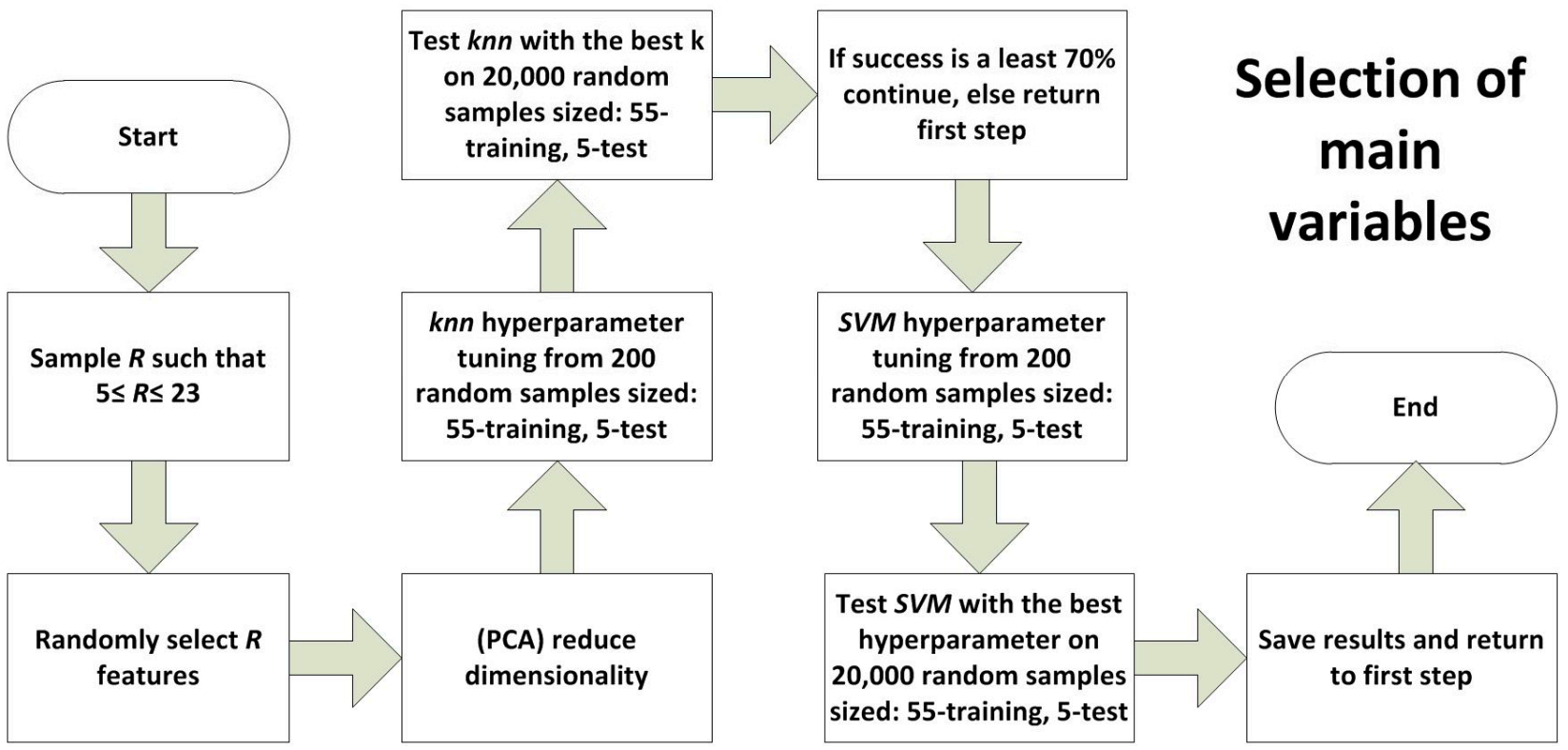
• Sample R such that 5 ≤ R ≤ 23 and randomly select R features: A random number R is obtained between 5 and 23. Next, R variables are chosen at random from among the 28 possible ones;
• Principal Component Analysis (PCA) to Reduce dimensionality: Subsequently, principal component analysis is applied, saving the first variables that explain more than 99.5% of the variance of the data. Therefore, from now on, we work with 60 individuals explained in at most R new variables;
• KNN hyperparameter tuning from 200 random samples sized 55-training and 5-test, test KNN with the best K on 20,000 random samples sized 55-training and 5-test: As we were interested in obtaining a good classification, the optimal number of neighbors k was sought, choosing between 1 and 10, starting from the one that offers the best results when applied in 200 random samples of size 55-training, 5-test. Once k has been obtained, the percentage of success with KNN is now estimated from 20,000 random samples of size 55-training, 5-test. Finally, the proportion of bad classifications related to group 3 is noted. If the percentage of success with KNN is less strict than 70%, step 1 becomes:
• SVM hyperparameter tuning from 200 random samples sized 55-training, 5-test: Now, exceeding 70% of success with KNN, SVM is applied taking into account the following parameters:

  ○

  Core: function in charge of transporting the data to a higher dimension where a better separation of the same can be achieved. Sigmoidal, polynomial, and Gaussian functions and the linear core were taken into account for the experiment;

  ○

  Penalty parameter C: it is an indicator of the error that one is willing to tolerate. The values for C of 10, 50, 75, and 100 were taken into account for the experiment;

  ○

  Gamma: indicates how far the points are taken into account when drawing up the separating boundary. The gamma values of 1, 0.8, 0.6, 0.4, 0.1, 0.01, and 0.001 were taken into account for the experiment;

  ○

  Degree: degree of the function in the polynomial nucleus. Grades 1, 2, 3, and 4 were taken into account for the experiment;

  ○

  Based on these parameters, a search was done among all the possible combinations in order to calculate which one of them offered the best results applied to 200 random samples of size 55-training, 5-test. GridSearchCV was used to perform the above task.

• Test SVM with the best hyperparameters on 20,000 random samples sized 55-training 5-test: Once the ideal combination has been obtained, the efficacy of SVM is estimated running the supervised method based on these parameters and applied to 20,000 random samples of size 55-training, 5-test. Hit and misclassification ratios related to group 3 are saved;
• Save results and return to first step: Back to step 1.

For sufficiently wide data collection, it was necessary to run the previous process in Python for around 40 h to obtain 1800 iterations, of which 250 corresponded to those cases where KNN and SVM were calculated at the same time (since KNN achieved more than 70% of success).

The data available was 60 cells, which supposed very little information with which to carry out the study. This influenced the search for the best parameters for KNN and SVM, since Cross Validation was not applied (the best parameters would hardly be obtained). Instead, a search based on 200 random samples of size 55-train, 5-test was applied.

Considering the results obtained, it could be concluded that the variables 4, 5, 8, 10, 13, 17, 19, 20, and 24 offered good global results as well as low error rates when making classifications related to group 3. Hence, those variables have been selected as representative ones, and it reduced the number of them from 9 to 7 by applying PCA (saving the first variables that explain more than 99.5% of the variance of the data). Afterward, groups of 55 cells were made again to train each model, and it was validated with the 4 remaining classifiers in each case. The classifiers to be tested were the following: KNN, SVM, RF, and MLP. On the other hand, CNN was also tested. Nevertheless, this classifier did not follow the same strategy as the four algorithms mentioned before (it directly used the 60, 113 × 113 matrix as input data). These models were chosen and compared since they are the most used in classification [30,31,32].

Below are included some details of the architecture of the models used. KNN and SVM architectures have already been described in the previous paragraphs, in which the representative variables selection was detailed. The number of neighbors considered in KNN was equal to the number of them obtained in the previous algorithm when the representative variables were selected. The same occurred with the hyperparameters obtained in SVM.

According to RF, each classifier was built based on 500 trees. Additionally, hyperparameter tuning was applied, combining the following parameters:

• Maximum depth: represents the maximum number of levels allowed in each decision tree. The values 20, 40, 60, 80, and 100 were taken into account;
• Minimum points per node: this is the minimum number of data allowed in each partition. The values 1, 2, 3, 4, and 5 were taken into account.
• Maximum variables: indicates the maximum number of variables (chosen at random) that are taken into consideration when partitioning a node. Usually, √n is used as a standard parameter, where n is the number of total variables, but √n − 1, √n, and √n + 1 were taken into account.

In the case of MLP, the model was built from an input layer made up of 7 neurons (coinciding with the dimensionality of the data), a first hidden layer made up of 128 neurons, a second hidden layer made up of 64 neurons, and an output layer made up of only 3 neurons (matching the number of classifications). The neural network created was dense, a network formed by neurons that were each connected to all possible neurons belonging to contiguous layers. The activator used in the process was the rectifier or ReLU activator, except in the last layer where the softmax function was used. In addition, hyperparameter tuning was applied, taking into account the following parameters:

• Epochs: indicates the number of times that the neural network reads the data from the training sample in order to adjust to them (translated into a successive update of its parameters). The values 25, 50, 75, 100, 150, and 200 were taken into account;
• Batches: indicates the speed with which the network parameters are updated as the epochs progress. The values 15, 25, 50, 75, 100, 150, and 200 were taken into account.

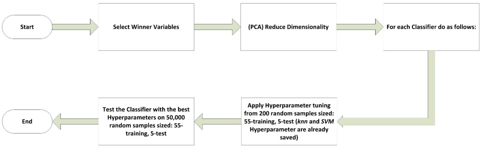
For the validation of the different models and obtaining the results, the methodology used with each of the 4 classifiers is shown in Figure 5.

In the case of CNN, it was built with a similar approach to the MLP. In order to find enough patterns to solve this problem, we have used a convolutional layer with 64 filters and a kernel size of 3 × 3. As to reduce the dimensionality, we also used a maxpool layer. Finally, a dense layer of 128 was introduced. In this architecture, we did not use dynamic parameter optimization. The networks need a high number of epochs to train (around 1000). We use the Nadam Optimizer [33] since it is the best in the tests that we have executed. We also exploit early-stopping, stopping the training when we do not have obtained better results in a certain number of epochs.

For the validation of the different models and obtaining the results, the methodology used with each of the five classifiers was as follows:

• For KNN and SVM:

  a.

  Test the classifier with the best hyperparameters (previously calculated) on 50,000 random samples sized: 55-training, 5-test.

• For RF and MLP:

  a.

  Apply hyperparameter tuning from 200 random samples sized: 55-training and 5-test.

  b.

  Test the classifier with the best hyperparameters on 50,000 random samples sized: 55-training and 5-test.

• For CNN:

  a.

  Test the classifier with the best hyperparameters (manually settled) on 100 random samples sized: 55-training and 5-test.

3. Results and Discussion

This section provides a concise description of the experimental results, their interpretation, as well as the discussion of the results and how they can be interpreted.

3.1. Justification of the Correct Initial Power Rating

As already mentioned, SOM was used to have some idea of whether the power classification was correct.

Next, Figure 6 shows four maps obtained considering the data with the representative variables previously obtained. Each pixel represented one of the 400 possible output neurons. Nearby pixels with dark values reflect proximity to each other, while nearby pixels with the contrast between light and dark representing distance. The elements of group 1 are represented in red, the elements of group 2 in green, and the elements of group 3 in blue.

Observing the results, it was possible to determine the existence of a certain grouping between the elements of the same color, and therefore of the same group. It was possible to conclude that the classification based on power was correct. Within group 3, it was deduced by the white border that the cells that are most distinguished from the rest of the groups were number 1, 4, and 6. Furthermore, comparing group 1 and 2, it could be concluded that it was easier to make a mistake when classifying cells from group 2 (green) in group 1 (red) than otherwise. This was due to the fact that some green points were mixed within the main mass of red points, which did not happen in the green group, where its elements had hardly any red elements inside them, except for element 0. Similarly, when classifying elements of group 3, it was possible to make a certain mistake and to identify them as elements of group 2, or vice versa, due to their greater closeness (compared to group 1). This could be verified by observing the results of the classifications, which will be shown later.

3.2. Classification of Variables

As already mentioned, the detection of the most important variables for the training of the models is crucial. To do this, it was necessary to run the previous process in Python for 40 h to obtain 1800 iterations, of which 250 iterations correspond to those cases where KNN and SVM were calculated at the same time.

Next,

Table 1. Relationship between success in classification and variables used.

	KNN Success	SVM Success	KNN + SVM Success Group 3	KNN Success Group 3	SVM Success Group 3	Variables
Top 1 KNN success	0.745	0.756	1.425	0.734	0.691	2, 4, 5, 7, 10, 13, 16, 17, and 22
Top 1 SVM success	0.7077	0.7628	1.5973	0.6975	0.8998	4, 5, 8, 10, 13, 17, 19, 20, and 24
Top 1 KNN + SVM success group 3	0.7005	0.7187	1.7646	0.9093	0.8552	2, 4, 6, 8, 10, 20, 23, and 24
Top 1 KNN success group 3	0.7095	0.7187	1.7646	0.9093	0.8552	2, 4, 6, 8, 10, 20, 23, and 24
Top 1 SVM success group 3	0.7099	0.7401	1.6371	0.704	0.9331	2, 4, 5, 7, 8, 9, 10, 12, 15, 16, 17, 18, 19, 20, and 21

shows the best results obtained according to different criteria, such as the success in the classification with KNN and SVM (columns 1 and 2), and proportion of bad classifications caused between groups 1 and 2 with respect to group 3, using KNN and SVM respectively (columns 4 and 5). Therefore, the value 0.9331 in row 5 and column 5 was interpreted by associating 93.331% to the percentage of bad classifications (applying SVM with the indicated variables) that were not related to group 3, to which only 6.669% corresponded. Therefore, a high proportion represented a smaller error in the classification of elements related to group 3. The third column is the sum of the fourth and fifth columns.

In addition, the frequency of appearance of each of the 28 variables in all the iterations (1800 in total) was studied based on two criteria:

• Success with KNN greater than 68.5% (seventy-fifth percentile);
• The proportion of bad classifications not related to group 3 higher than 79.4% (eighty-fifth percentile).

From the first criteria, it was deduced that good candidate variables were 2, 4, 5, and 7 whereas bad candidate variables were 1, 3, 6, 26, 27, and 28. From the second criteria, it was concluded that good candidate variables were 2, 4, 6, 23, and 28 whereas bad candidate variables were 1, 7, 25, and 27. Comparing the results obtained, it was possible to conclude that there was a relationship between the importance of a variable and its frequency of appearance following the two criteria mentioned.

The same type of criteria could be considered for SVM. However, it was possible that given the low number of iterations (250), the results were not entirely reliable.

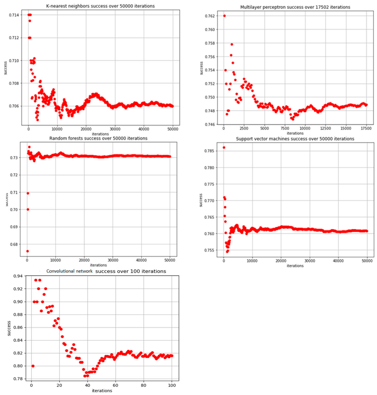
3.3. Convergence and Results of the Models

An important aspect when working with AI is the convergence of the model. Next, Figure 7 shows the behavior of the hit obtained with each of the classifiers, depending on the number of iterations performed. In the case of MLP, 50,000 iterations were not reached due to the high computational cost, although there was no loss of efficiency, as was well observed in all models since there was some convergence at a lower number of iterations.

In the CNN model compilation appeared a critical problem. The amount of time needed to finish one iteration was extremely high. This was vital in order to decide the number of iterations. The authors finally decided to use 100 iterations of 1000 epochs. With this number of iterations, some convergence was obtained.

From the results shown in Figure 7, the most successful model from the first fourth classifiers (KNN, SVM, RF, and MLP) was SVM, closely followed by MLP and RF. The worst result was obtained by KNN; however, the success rate was 70.61%, and it was possible to consider it as being of high value. On the other hand, it could be seen that the fifth classifier, CNN, achieved higher success than the rest, exceeding 80%.

Table 2. Classification results in the five models.

	Classification Success	Time Spent on Hyperparameter Tuning (hr)	Time Spent Testing 50,000 (17,502 with MLP/100 CNN) Samples (hr)
KNN	0.7061	0.0017	0.0267
SVM	0.7607	0.0223	0.0196
RF	0.7308	2.1552	8.8071
MLP	0.7488	0.9633	15.5442
CNN	0.8160		100

shows the results (percentage of success) of the five models used once the cells used for the validation phase were classified. The time (hours) required are also shown. With regard to time, the first column of times shows the time needed to locate the ideal parameters (hyperparameter tuning), while the second column of times indicates the time needed for classifier training.

Regarding the time spent in locating the main parameters, the fastest model was KNN, with SVM following and with a time close to 1 h, MLP. RF presented the worst time to locate these parameters, requiring more than 2 h.

Regarding the time spent on training, SVM was the fastest, closely followed by KNN. At the other extreme, RF required almost 9 h, followed by MLP with 15.54 h, and CNN with 100 h.

Observing results presented in Table 2, it could be concluded that CNN presented the highest percentage of success, with 81.6% but was also extremely slow (around 100 h). SVM was the model that presented the second-highest efficiency (76.07%), and it was the model with reasonably lower times (search for parameters and training).

One of the main goals of sorting was to detect bad cells (group 3). In this sense,

Table 3. Group 3 classification results and results of misclassification between groups.

	Success on Group 3	1 Missclassified as 2	1 Missclassified as 3	2 Missclassified as 1	2 Missclassified as 3	3 Missclassified as 1	3 Missclassified as 2
KNN	0.7002	0.1017	0	0.5985	0.0117	0.0579	0.2302
SVM	0.9055	0.1377	0.0077	0.7678	0.0142	0.0044	0.0752
RF	0.7746	0.2525	0	0.5221	0.0142	0.0173	0.1939
MLP	0.8224	0.2166	0.0018	0.6058	0.0687	0.0073	0.0998
CNN	0.6956	0.2282	0.0217	0.3586	0.0865	0.0543	0.25

shows the results of the classification of cells in group 3. In the same way, Table 3 shows the results of the misclassification between groups.

Focusing only on the classification of group 3, SVM obtains success results of 90.55%, while MLP obtains 82.24%, RF obtains 77.46%, KNN 70.02%, and the worst result is for CNN with 69.56%.

It could also be observed that there was hardly any confusion between cells of group 1 with group 3 or cells of group 2 with group 3. In the first case, KNN and RF did not present confusion (0%), while MLP, SVM, and CNN presented 0.18%, 0.77%, and 2.17%, respectively. In the second case, KNN, SVM, and RF presented a value below 1.5%, while MLP presented a value of 6.87% and CNN the highest value, 8.65%.

Greater confusion appears between groups 1 and 2. As can be seen, the misclassification of cells in group 1 as group 2 varied between 10.17% for KNN and 25.25% for RF. In the case of misclassification of cells in group 2 to group 1 was when the CNN performed better than the other algorithms, with 35.86% for CNN, reaching 76.78% in the case of SVM. This inaccuracy was due to the similarity between some cells, as can be seen in Figure 6.

4. Conclusions

The work presents different solar PV cell defect classifiers, using five different classifier models, KNN, SVM, RF, MLP, and CNN. The classification was carried out based on EL images and I-V curves, all of them at the solar PV cell level. For all cases, good classification was obtained, and the differences between the proposed models were analyzed. CNN presented the highest percentage of success, with 81.6%, but it was also extremely slow (around 100 h). SVM was the model that presented the second-highest efficiency (76.07%), and it was the model with a reasonably short computation time.

The classifiers’ biggest application is in defective solar PV cells classification. Furthermore, this group of cells is the one of greatest interest since it is the group that contains cells with almost zero electrical production. The work also presents a method to be used to select variables of interest, which will serve to train the different models of the classifiers. This process is essential since the use of variables without relevance can cause noise in training and the consequent obtaining of bad results in the classification.

The study has focused on PV solar cells from a single PV solar module. As future work, it is proposed that the dataset should be extended, and the evaluation of how this extension improves the results in each of the five models should be evaluated. We will also work on collecting data from individual cells (isolated, which are not part of a module) to expand the dataset in the future. We are also going to explore the option of generating synthetic data with GAN networks. The authors will also work on collecting data from isolated individual PV cells (which are not part of a module) to expand the dataset in the future. We are also going to explore the option of generating synthetic data with GAN networks. The authors will also extend this work, applying the classification to PV solar cells to other modules. Testing IRT image-based classifiers and IRT and EL image classifiers together are also proposed as future works. This work is of interest as it is known that both techniques are complementary in certain aspects. Another application of AI in which authors are working is the estimation of the I-V curve from EL images and IRT, at the level of the solar PV module.

References

1. Scholten, D.; Bazilian, M.; Overland, I.; Westphal, K. The geopolitics of renewables: New board, new game. Energy Policy 2020, 138, 111059. [Google Scholar] [CrossRef]
2. Gugler, K.; Haxhimusa, A.; Liebensteiner, M.; Schindler, N. Investment opportunities, uncertainty, and renewables in European electricity markets. Energy Econ. 2020, 85, 104575. [Google Scholar] [CrossRef]
3. REN21. Renewables 2020 Global Status Report; REN21 Secretariat: Paris, France, 2020; ISBN 978-3-948393-00-7. Available online: http://www.ren21.net/gsr-2020/ (accessed on 15 January 2021).
4. Behzadi, A.; Arabkoohsar, A. Feasibility study of a smart building energy system comprising solar PV/T panels and a heat storage unit. Energy 2020, 210, 118528. [Google Scholar] [CrossRef]
5. Fachrizal, R.; Ramadhani, U.H.; Munkhammar, J.; Widén, J. Combined PV–EV hosting capacity assessment for a residential LV distribution grid with smart EV charging and PV curtailment. Sustain. Energy Grids Netw. 2021, 26, 100445. [Google Scholar] [CrossRef]
6. Thornbush, M.; Golubchikov, O. Smart energy cities: The evolution of the city-energy-sustainability nexus. Environ. Dev. 2021, 100626, 100626. [Google Scholar] [CrossRef]
7. Hernández-Callejo, L.; Gallardo-Saavedra, S.; Alonso-Gómez, V. A review of photovoltaic systems: Design, operation and maintenance. Sol. Energy 2019, 188, 426–440. [Google Scholar] [CrossRef]
8. Gallardo-Saavedra, S.; Hernández-Callejo, L.; Duque-Pérez, O. Quantitative failure rates and modes analysis in photovoltaic plants. Energy 2019, 183, 825–836. [Google Scholar] [CrossRef]
9. Gallardo-Saavedra, S.; Hernández-Callejo, L.; Alonso-García, M.D.C.; Santos, J.D.; Morales-Aragonés, J.I.; Alonso-Gómez, V.; Moretón-Fernández, Á.; González-Rebollo, M.A.; Martínez-Sacristán, O. Nondestructive characterization of solar PV cells defects by means of electroluminescence, infrared thermography, I–V curves and visual tests: Experimental study and comparison. Energy 2020, 205, 117930. [Google Scholar] [CrossRef]
10. Blakesley, J.C.; Castro, F.A.; Koutsourakis, G.; Laudani, A.; Lozito, G.M.; Fulginei, F.R. Towards non-destructive individual cell I-V characteristic curve extraction from photovoltaic module measurements. Sol. Energy 2020, 202, 342–357. [Google Scholar] [CrossRef]
11. Morales-Aragonés, J.; Gallardo-Saavedra, S.; Alonso-Gómez, V.; Sánchez-Pacheco, F.; González, M.; Martínez, O.; Muñoz-García, M.; Alonso-García, M.; Hernández-Callejo, L. Low-cost electronics for online i-v tracing at photovoltaic module level: Development of two strategies and comparison between them. Electronics 2021, 10, 671. [Google Scholar] [CrossRef]
12. Morales-Aragonés, J.; Alonso-García, M.; Gallardo-Saavedra, S.; Alonso-Gómez, V.; Balenzategui, J.; Redondo-Plaza, A.; Hernández-Callejo, L. Online distributed measurement of dark i-v curves in photovoltaic plants. Appl. Sci. 2021, 11, 1924. [Google Scholar] [CrossRef]
13. Jordan, D.C.; Silverman, T.J.; Wohlgemuth, J.H.; Kurtz, S.R.; VanSant, K.T. Photovoltaic failure and degradation modes. Prog. Photovolt. Res. Appl. 2017, 25, 318–326. [Google Scholar] [CrossRef]
14. Gallardo-Saavedra, S.; Hernández-Callejo, L.; Duque-Perez, O. Technological review of the instrumentation used in aerial thermographic inspection of photovoltaic plants. Renew. Sustain. Energy Rev. 2018, 93, 566–579. [Google Scholar] [CrossRef]
15. Gallardo-Saavedra, S.; Hernandez-Callejo, L.; Duque-Perez, O.; Hermandez, L. Image resolution influence in aerial thermographic inspections of photovoltaic plants. IEEE Trans. Ind. Inform. 2018, 14, 5678–5686. [Google Scholar] [CrossRef]
16. Ballestín-Fuertes, J.; Muñoz-Cruzado-Alba, J.; Sanz-Osorio, J.F.; Hernández-Callejo, L.; Alonso-Gómez, V.; Morales-Aragones, J.I.; Gallardo-Saavedra, S.; Martínez-Sacristan, O.; Moretón-Fernández, Á. Novel utility-scale photovoltaic plant electroluminescence maintenance technique by means of bidirectional power inverter controller. Appl. Sci. 2020, 10, 3084. [Google Scholar] [CrossRef]
17. Gligor, A.; Dumitru, C.-D.; Grif, H.-S. Artificial intelligence solution for managing a photovoltaic energy production unit. Procedia Manuf. 2018, 22, 626–633. [Google Scholar] [CrossRef]
18. Wang, H.; Liu, Y.; Zhou, B.; Li, C.; Cao, G.; Voropai, N.; Barakhtenko, E. Taxonomy research of artificial intelligence for deterministic solar power forecasting. Energy Convers. Manag. 2020, 214, 112909. [Google Scholar] [CrossRef]
19. Kayri, I.; Gencoglu, M.T. Predicting power production from a photovoltaic panel through artificial neural networks using atmospheric indicators. Neural Comput. Appl. 2017, 31, 3573–3586. [Google Scholar] [CrossRef]
20. Li, L.-L.; Wen, S.-Y.; Tseng, M.-L.; Chiu, A.S.F. Photovoltaic array prediction on short-term output power method in centralized power generation system. Ann. Oper. Res. 2018, 290, 243–263. [Google Scholar] [CrossRef]
21. Hussain, M.; Dhimish, M.; Titarenko, S.; Mather, P. Artificial neural network based photovoltaic fault detection algorithm integrating two bi-directional input parameters. Renew. Energy 2020, 155, 1272–1292. [Google Scholar] [CrossRef]
22. Cho, K.-H.; Jo, H.-C.; Kim, E.-S.; Park, H.-A.; Park, J.H. Failure diagnosis method of photovoltaic generator using support vector machine. J. Electr. Eng. Technol. 2020, 15, 1669–1680. [Google Scholar] [CrossRef]
23. Pérez-Romero, Á.; Hernández-Callejo, L.; Gallardo-Saavedra, S.; Alonso-Gómez, V.; Alonso-García, M.d.C.; Mateo-Romero, H.F. Photovoltaic cell defect classifier: A model comparison. In Proceedings of the III Ibero-American Conference on Smart Cities, San José, Costa Rica, 9–11 November 2020; pp. 257–273. [Google Scholar]
24. Bishop, C.M. Pattern recognition and machine learning. In Information Science and Statistics; Springer: New York, NY, USA, 2006; pp. 21–24. ISBN 9780387310732. [Google Scholar]
25. Kohonen, T. Self-organized formation of topologically correct feature maps. Biol. Cybern. 1982, 43, 59–69. [Google Scholar] [CrossRef]
26. Kohonen, T. Self-Organization and Associative Memory, 2nd ed.; Springer: Berlin/Heidelberg, Germany, 1988; ISBN 978-3540183143. [Google Scholar]
27. Rumelhart, D.E.; Hinton, G.E.; Williams, R.J. Learning representations by back-propagating errors. Nature 1986, 323, 533–536. [Google Scholar] [CrossRef]
28. Silverman, B.W.; Jones, M.C.; Fix, E. An important contribution to nonparametric discriminant analysis and density estimation: Commentary on fix and hodges (1951). Int. Stat. Rev. 1989, 57, 233. [Google Scholar] [CrossRef]
29. Kohonen, T. Self-Organizing Maps; Springer Series in Information Sciences: Berlin/Heidelberg, Germany, 2001; Volume 30, ISBN 978-3-540-67921-9. [Google Scholar]
30. Kothari, S.; Oh, H. Neural networks for pattern recognition. Adv. Comput. 1993, 37, 119–166. [Google Scholar] [CrossRef]
31. Clancey, W.J. Heuristic classification. Artif. Intell. 1985, 27, 289–350. [Google Scholar] [CrossRef]
32. Rodrigues, M.A. Invariants for Pattern Recognition and Classification. In Ensemble Learning; World Scientific: Singapore, 2000; Volume 42. [Google Scholar]
33. Dozat, T. Incorporating Nesterov Momentum into Adam; ICLR Work: Paris, France, 2016; pp. 1–4. [Google Scholar]
Figure 1. (a) Front view of the module. (b) Back view of the module.
Applsci 11 04226 g001
Figure 2. EL image and cell numbering for model training.
Applsci 11 04226 g002
Figure 3. Pseudocode of the procedure for selecting the most significant variables.
Applsci 11 04226 g003
Figure 4. Proposed methodology for the selection of main variables.
Applsci 11 04226 g004
Figure 5. Methodology used with each of the 4 classifiers.
Applsci 11 04226 g005
Figure 6. Result when applying SOM to the available data [23].
Applsci 11 04226 g006
Figure 7. Comparison of classification success versus the number of iterations for the five models [23] and authors elaboration.
Applsci 11 04226 g007