Activity Recognition with Combination of Deeply Learned Visual Attention and Pose Estimation

Abstract

While human activity recognition and pose estimation are closely related, these two issues are usually treated as separate tasks. In this thesis, two-dimension and three-dimension pose estimation is obtained for human activity recognition in a video sequence, and final activity is determined by combining it with an activity algorithm with visual attention. Two problems can be solved efficiently using a single architecture. It is also shown that end-to-end optimization leads to much higher accuracy than separated learning. The proposed architecture can be trained seamlessly with different categories of data. For visual attention, soft visual attention is used, and a multilayer recurrent neural network using long short term memory that can be used both temporally and spatially is used. The image, pose estimated skeleton, and RGB-based activity recognition data are all synthesized to determine the final activity to increase reliability. Visual attention evaluates the model in UCF-11 (Youtube Action), HMDB-51 and Hollywood2 data sets, and analyzes how to focus according to the scene and task the model is performing. Pose estimation and activity recognition are tested and analyzed on MPII, Human3.6M, Penn Action and NTU data sets. Test results are Penn Action 98.9%, NTU 87.9%, and NW-UCLA 88.6%.

1. Introduction

Human activity recognition and pose estimation have attracted many applications such as video-based recognition and human–computer interfaces. However, in terms of accuracy and speed, a lot of research is still being conducted. Activity recognition and pose estimation are usually handled separately. Despite the fact that pose is very related to activity recognition, for the advantage of activity recognition, a method of solving both problems at once is not actively studied [1]. Therefore, this paper focuses on a unique end-to-end deep learning algorithm for jointly processing two-dimensional (2D) and three-dimensional (3D) human activity recognition and pose estimation.

One of the main advantages of deep learning is that it can perform end-to-end optimization. As suggested by Kokkinos et al. [2], there are many advantages in the case of a deep learning problem that can perform end-to-end optimization. Recent methods based on deep convolutional neural networks have obtained results with high accuracy in both 2D and 3D pose estimation tasks thanks to the advent of a new architecture and the availability of large amounts of data [3]. Similarly, activity recognition has recently been improved using deep neural networks that depend on human pose [4]. Since most of the pose estimation methods perform heat map prediction, the two tasks have yet to be combined and joint optimization has not been performed. This detection-based approach requires a function that maximizes the value to recover the joint coordinates as a post-processing step, which breaks the backpropagation loop required for end-to-end learning. Therefore, if this problem is solved, the pose estimation method and the activity recognition method, which are very closely related, can be processed together to achieve higher accuracy. When learning is performed using RGB-based image data and activity recognition is performed, it is difficult to distinguish very similar activity such as drinking water or receiving a phone call. However, in pose estimation, it is possible to know that the pose is clearly different using the joints of the body, and if the activity recognition is performed using this joint data, the activity can be more accurately recognized.

Performing human activity recognition using deep learning made learning by imitating human neural networks. However, it is known that human visual recognition does not focus on the entire scene at once [5]. Instead, humans focus sequentially on different parts of the scene to extract relevant information. Most of the existing computer vision algorithms do not use an attention mechanism and are not actively studied in various fields of image/video. With the recent surge in deep neural networks, attention-based models have been shown to achieve promising results in several challenging tasks including subtitle generation, machine translation, and games. Many of these models use RNN (Recurrent Neural Network)-based Long Short Term Memory (LSTM) and show good results in the training sequence. The visual attention model can be classified into a soft attention model and a hard attention model [6]. Soft attention models are deterministic and can be trained using backpropagation, while hard attention models are probabilistic and are trained with reinforcement learning algorithms [7]. Hard attention models can be computationally expensive because they require sampling when training. On the other hand, in the soft-attended approach, differentiable mappings can be used from any positional output to the next input. Therefore, the computational amount is less than that of hardattention models. The attention-based model can potentially infer activity occurring in the video by focusing only on the relevant position of each frame. Therefore, in this paper, we propose a final activity recognition algorithm in which the soft visual attention model is preceded, the weight is increased to the relevant location, and the activity is recognized using visual data, and the data through pose estimation are considered together. Related work to the proposed work in this paper is presented in

Table 1. Comparison with other methods.

	Purpose	Feature	Difference
Wang et al. [8]	Sitting posture recognition	Pose estimation Sitting pose	Visual attention and activity recognition are performed with pose estimation Performing not only sitting pose but also other poses
Nadeem et al. [9]	Posture estimation for sport activity recognition	Pose estimation for activity recognition Entropy markov model	Visual attention is also additionally combined to perform Activity recognition is performed by combining it with an end-to-end model
Kulikajevas et al. [10]	Detection of sitting posture	pose estimation Sitting pose	Visual attention and activity recognition are performed with pose estimation Performing not only sitting pose but also other poses
Proposed	Activity recognition with combination of deeply learned visual attention and pose estimation	Pose estimation, visual attention, activity recognition 60 activities	Visual attention, pose estimation, and appearance based activity recognition are performed

.

2. Related Work

2.1. Visual Attention

Convolutional neural network (CNN) has been very successful in image classification and object recognition [11]. Classifying videos instead of images adds a temporal dimension to the image classification problem. Learning temporal dynamics is a difficult problem, and previous approaches use optical flow, Histogram of Gradient (HOG), and hand-crafted features to generate appearances and a variety of information-encoded descriptors. LSTM has recently been shown to show high recognition performance in the areas of speech recognition, machine translation, image description, and video description [12,13]. In addition, many studies have begun on LSTM based on high recognition performance in activity recognition [14]. Most existing activity recognition methods tend to classify sequences directly with CNN, which is the basis of LSTM, or perform temporal pooling of features before classification [15]. In addition, LSTM was used in the encoder-decoder framework to learn effective representation of video in an unsupervised setting using video. Recently, Yao et al. [14] proposed to generate video description using 3D CNN function and LSTM decoder in the encoder-decoder framework. In this paper, we unify the focus on video by defining the probability distribution over the frames used to generate individual words. In general, analyzing the interior of a deep neural network is difficult because it is called a black box. However, when performing a specific task, the visual attention model adds a weight to the location where the model focuses to add interpretation possibilities. Karpathy et al. [16] performed behavior recognition in video using a multi-resolution CNN architecture. In this paper, the concept of center is mentioned and focus is focused on the center of the frame. Recent work by Xu et al. [17] generated image descriptions using both soft focus and hard focus mechanisms. Their model actually sees each object when creating the description. This paper is based on this model. However, Xu et al. [17] mainly worked on the caption generation of static images, and this paper focuses on using the soft attention mechanism for activity recognition in video. Recently, Jaderberg et al. [18] proposed a soft attention mechanism that adds a spatial converter module between CNN layers. Instead of weighting the position using the softmax layer that is performed, an affine transform was applied to several layers of the CNN to process the relevant parts, and experiments were conducted on the Street View House Numbers data set [19]. Yeung et al. [20] performed dense task labeling using a temporal attention-based model based on the input-output context and showed the result of helping a better understanding and higher accuracy of the temporal relationship of the working video. In Figure 1, a man is playing soccer with a ball. The image above is the original image, and the image below is the image with visual attention applied. The man and the ball are marked in white. The part marked in white is the part that has a higher weight by applying visual attention.

2.2. Activity Recognition

Activity recognition in video is considered a difficult problem because it contains a high level of description, and it is also difficult to deal with the temporal dimension easily. The previous approach used the classical method for feature extraction [21]. The key idea here is to use visual features in space and time using body joint position. 3D convolution has recently been mentioned as an option that provides the highest classification score [22]. However, it has a large number of parameters, and requires a large amount of memory for training. And we can’t use a lot of images efficiently. Activity recognition improves accuracy by a model focused on body parts, and a two-stream network can be used to merge RGB images and expensive optical flow maps [23]. Most 2D activity recognition methods use body joint information to extract visual features, similar to attention mechanisms. Some methods of directly exploring body joints do not create them and are therefore limited to datasets that provide skeleton data. The approach of this paper removes this limitation by performing pose estimation along with activity recognition. Therefore, the proposed model only needs RGB frames that are input as input while performing identifiable visual recognition according to the estimated body joints. Unlike video-based activity recognition, 3D activitiy recognition mainly uses skeleton data as basic information [24]. Depth sensors such as Microsoft Kinect can be used to capture 3D skeleton data without the complicated setup procedures required for a motion capture system (Mocap). However, due to the use of infrared projectors, these depth sensors are limited to indoor environments. In addition, since the range precision is low and it is not resistant to occlusion, noise often occurs in the skeleton. In order to cope with a noisy joint, the spatio/temporal LSTM network applied a gating mechanism to learn the reliability of the joint sequence or used an attention mechanism [25,26]. In addition to the skeleton data, the multi-mode approach can benefit from visual cues. In a similar way, Baradel et al. [27] proposed a spatio/temporal attention mechanism that represents a pose using joint sequences for both spatial and temporal attention mechanisms, and the activity classification is based on the pose and appearance features extracted by the same method. The architecture predicts high-precision 3D skeletons from the input RGB frames, so there is no need to post-process Kinect’s noisy skeletons. Also, in this paper, temporal convolution was used instead of the general LSTM. However, it shows excellent performance for 3D activity recognition.

2.3. Pose Estimation

The problem of human pose estimation is a field that has been continuously studied over the past few years, from image structure-based methods to recent CNN approaches [28,29]. Research related to pose estimation can be largely divided into two methods detection-based method and regression-based method. The detection-based method estimates the pose as a heat map prediction problem. Each pixel of the heat map represents the detection score of the corresponding joint [30]. Studying the concepts of stacked architecture, remaining connections and multi-scale processing, Newell et al. [3] proposed a stacked hourglass network, which significantly improved the accuracy of the 2D pose estimation problem. Since then, state-of-the-art methods have been proposing complex variations of the stacked hourglass architecture [3]. For example, in the study of CRF (Conditional Random Field) and Yang et al. [31], the residual unit was replaced by PRM (Pyramid Residual Module). GAN (Generative Adversarial Networks) was used to improve the heat map by improving the learning ability of structural information and learning predictions with high accuracy [32]. However, the detection approach does not directly provide joint coordinates. The function that maximizes the value to recover the posture from the (x, y) coordinate is usually applied as a post-processing step. The regression-based approach, on the other hand, uses a nonlinear function that maps the input directly to the desired output (joint coordinates). According to this paradigm, Toshev et al. [33] proposed dependent regression for body part detection and Carreira et al. [34] proposed repetitive error feedback. A limitation of the regression method is that the regression function is not frequently optimized. To solve these weaknesses, Luvizon et al. [35] proposed that the soft-maximum likelihood function can be converted directly from the heat map into joint coordinates, and consequently, the detection method can be converted into a regression method. The main advantage of regression methods over detection methods is that they are mostly completely distinguishable. This means that the output of the pose estimation can be used for further processing and the whole system can be modified little by little. In recent years, thanks to the availability of high-quality data, a deep architecture has been used to learn accurate 3D representations from RGB images, and it also outperforms depth sensors [36,37]. First, 2D pose estimation considering camera coordinates is processed, and second, the estimated pose is matched with 3D representation through nonparametric shape model. Skeletal representation of human pose has been proposed to reduce data variance, but this structural transformation can have a negative effect on tasks that depend on the skeleton of the human body because errors accumulate every time it moves away from the underlying skeleton [38]. Pavlakos et al. [39] proposed a stacked hourglass architecture. However, this method greatly increases the number of parameters and memory required to store all gradients. The approach of this paper also stores the representation of 3D pose, but uses a much lower resolution than the algorithm proposed by Pavlakos et al. [39] and uses much less memory by using the continuous regression function.

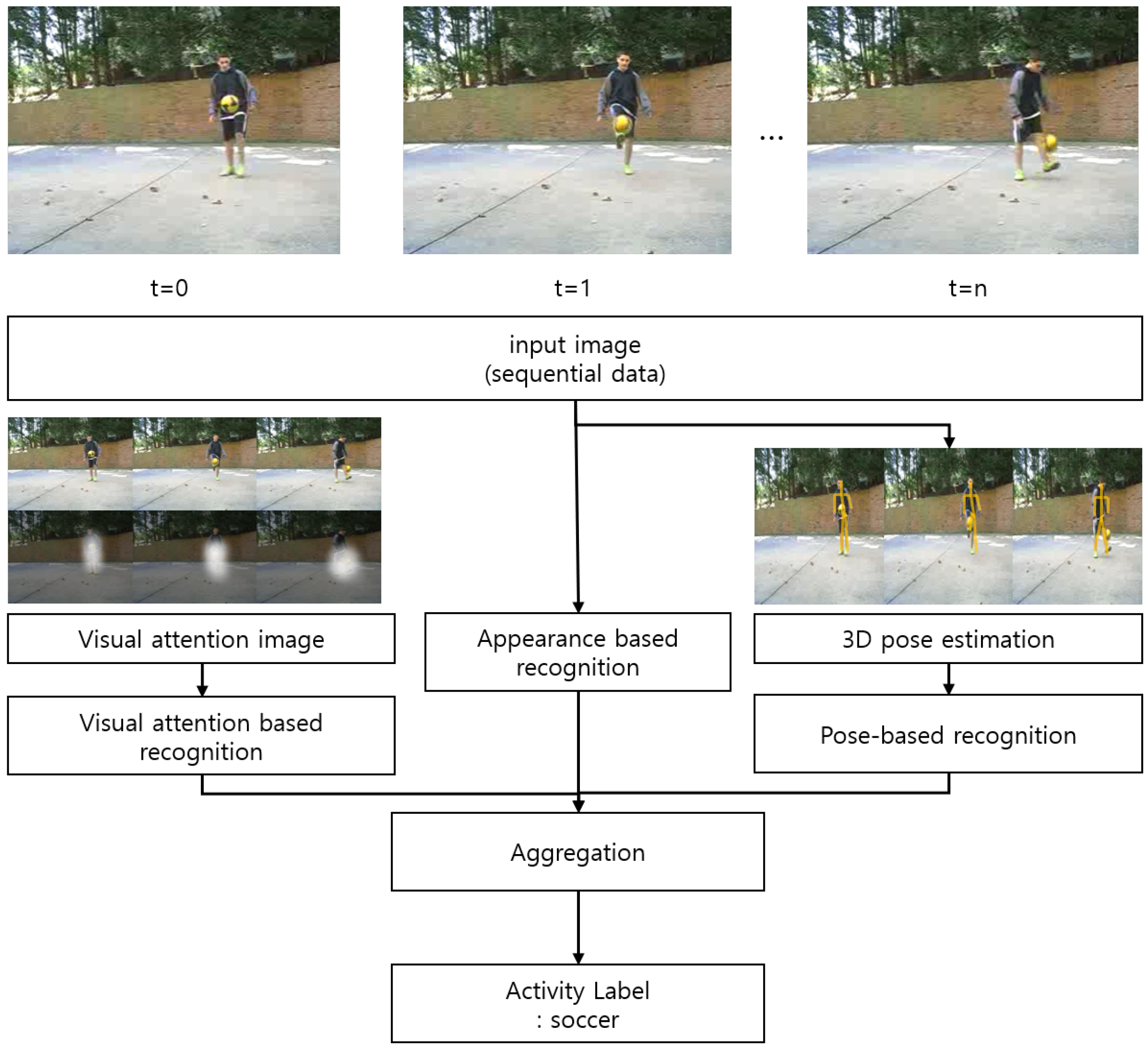
3. Proposed Algorithm

This section describes the detailed description of the proposed algorithm. As shown in Figure 2, input image is used by dividing the video sequentially. And visual attention is performed, and as a result, appearance based recognition is performed. The result of performing pose estimation using the input image is also combined with the previous result to select to final label. Activity recognition procedure is shown as pseudocode in Algorithm 1. Section 3.1 describes the visual attention algorithm in detail, and Section 3.2 describes pose estimation-based activity recognition in detail. And in Section 3.3, activity recognition is described in detail.

Algorithm 1 Activity recognition procedure.

Input: Video frame N Output: Result of activity 1: for Activity recognition do 2:     Visual attention based activity recognition (N) 3:     Pose estimation based activity recognition (N) 4:     Appearance based activity recognition (N) 5:     Aggregation 6: end for

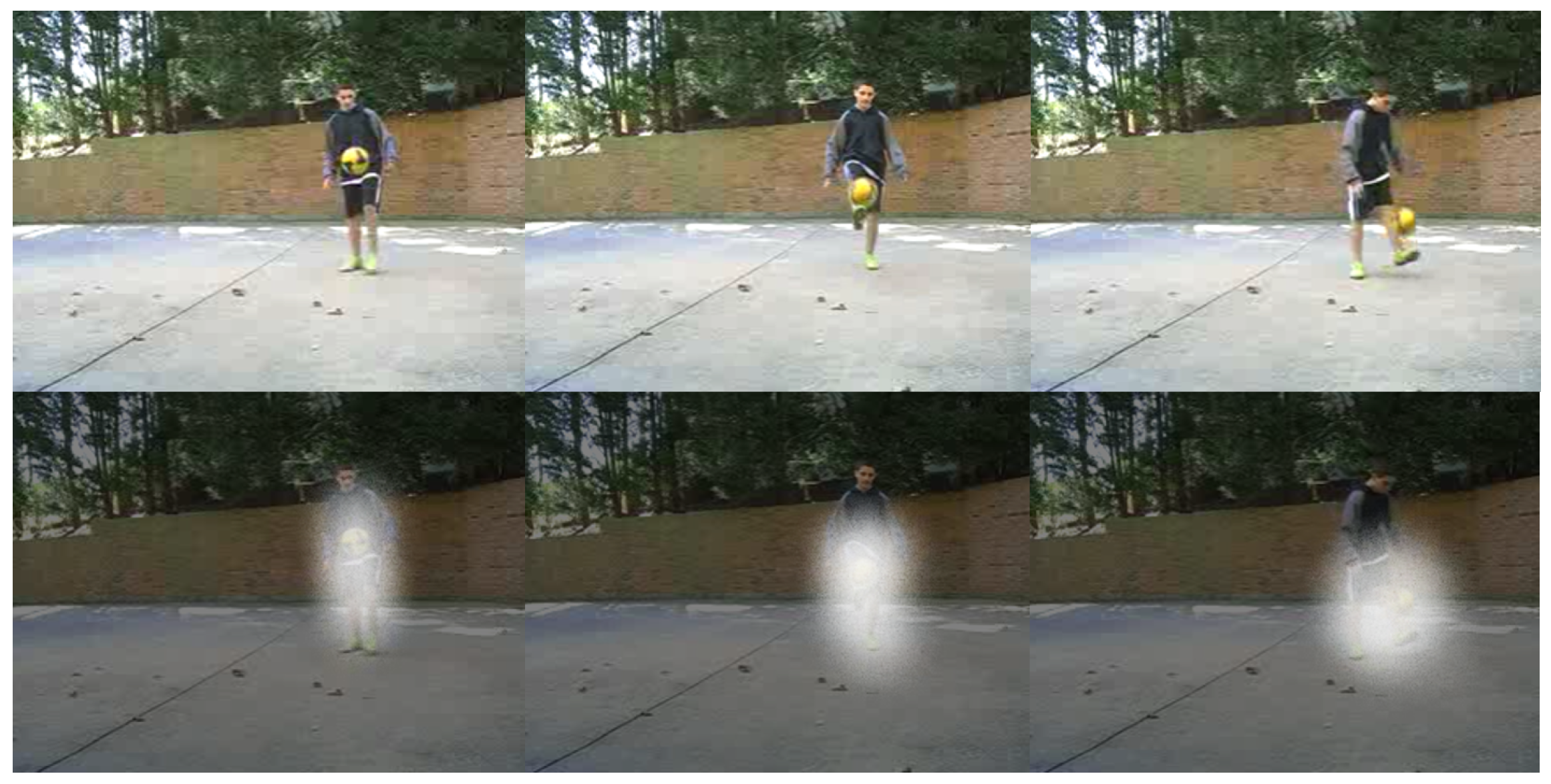
3.1. Visual Attention

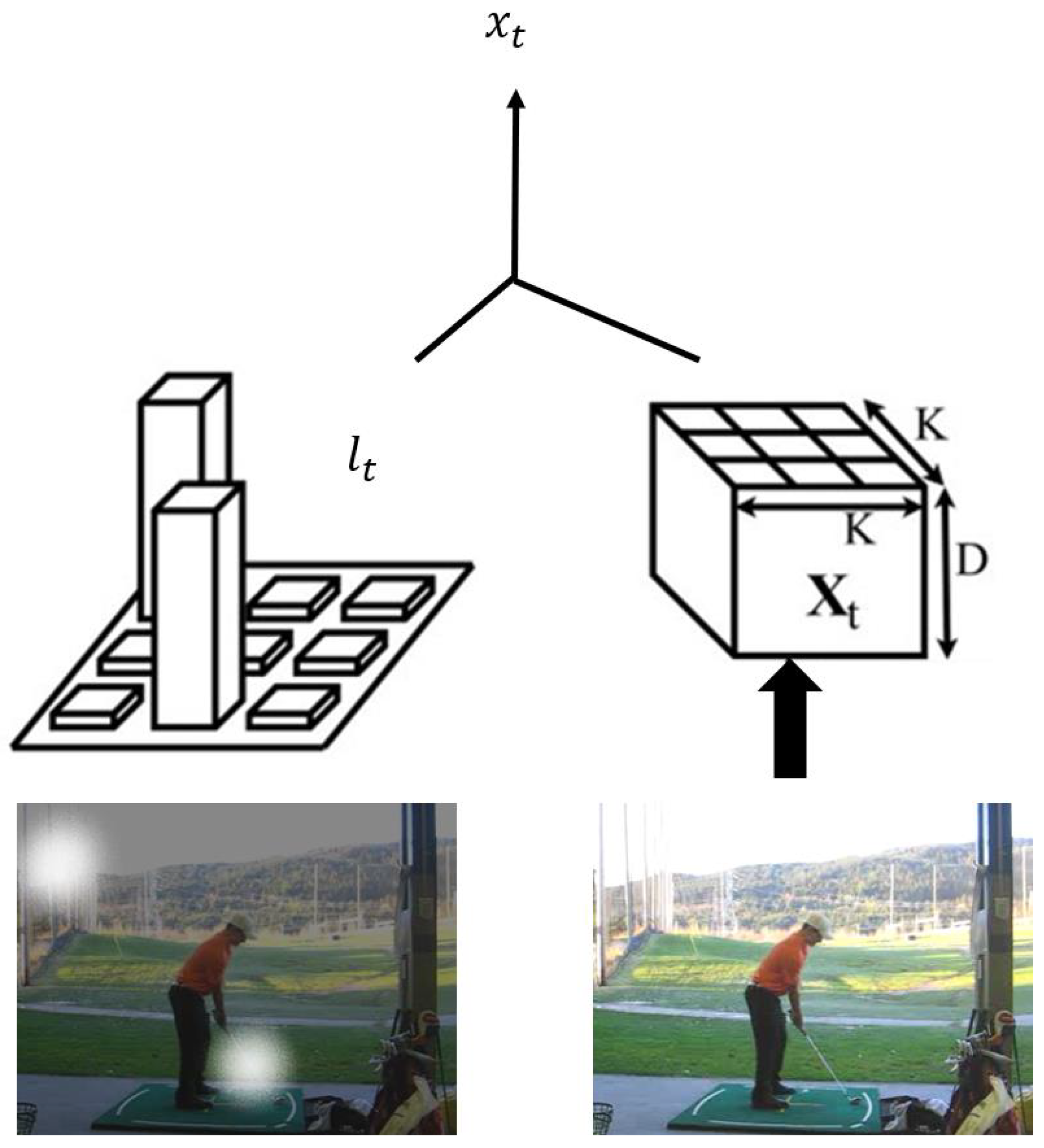
3.1.1. Convolutional Features

In this paper, we extract the last convolutional layer obtained by pushing video frames through the GoogLeNet model [40] trained on the ImageNet dataset [41]. This last convolutional layer has a D convolutional maps and is a feature cube of shape $K\times K\times D$ (7 × 7 × 1024 in our experiments). So, we extract $K^2$D-dimensional vectors. We refer to these vectors as feature slices in a feature cube:

$$X_t=[X_{t,1},\dots ,X_{t,K^2}],$$

(1)

$$X_{t,i}\in {\mathbb{R}}^D.$$

(2)

Each of these $K^2$ vertical feature slices mapped to a different overlapping region in the input space, and the model draws attention to these $K^2$ regions. $X_{t,i}$ refers to the i slice of the D-dimensional vector $X_t$.

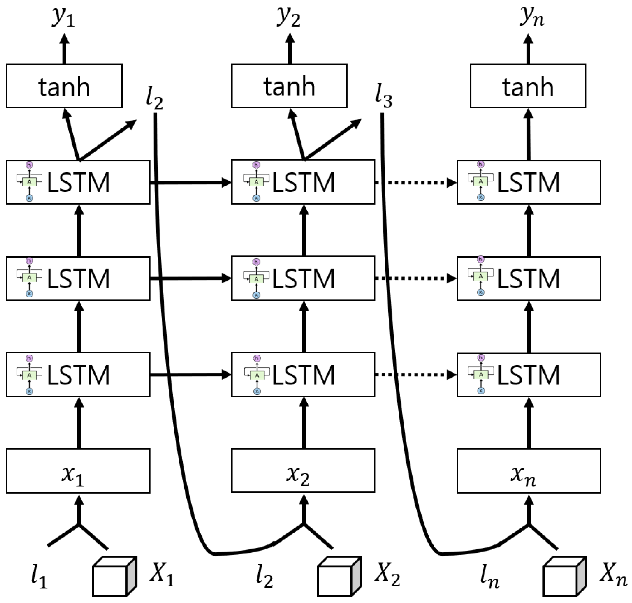
3.1.2. LSTM and Attention Mechanism

In this paper, we implemented using LSTM proposed by Xu et al. [17].

$$\left(\begin{array}{c}{i}_t\\ f_t\\ o_t\\ g_t\end{array}\right)=\left(\begin{array}{c}\sigma (W_i{x}_t+W_i{h}_{t-1}+b_i)\\ \sigma (W_f{x}_t+W_f{h}_{t-1}+b_f)\\ \sigma (W_o{x}_t+W_o{h}_{t-1}+b_0)\\ tanh(W_g{x}_t+W_g{h}_{t-1}+b_g\end{array}\right)M\left(\begin{array}{c}{h}_{t-1}\\ x_t\end{array}\right),$$

(3)

$$c_t=f_t\odot c_{t-1}+i_t\odot g_t,$$

(4)

$$h_t=o_t\odot tanh\left(c_t\right),$$

(5)

where $i_t$ is the t input gate, $f_t$ is the t forget gate, $o_t$ is the t output gate, and $g_t$ is t memory gate, and is calculated as shown in Equation (3). $\sigma (·)$ is the sigmoid function, and $\sigma \left(s\right)$ is defined as follows.

$$\sigma \left(s\right)=\frac{1}{1+e^{-s}},$$

(6)

$W_i{x}_t,W_f{x}_t,W_o{x}_t,W_g{x}_t,$ is 4 weights used in each gate of the t time with $x_t$, and $W_i{h}_{t-1},$$W_f{h}_{t-1},W_o{h}_{t-1},W_g{h}_{t-1}$ is the 4 weights used in each gate of the $t-1$ time with $h_{t-1}$. $b_i,b_f,b_o,b_g$ is 4 weights bias used in each gate. $c_t$ is the t cell state, $h_{t-1}$ is the $t-1$ hidden state, $x_t$ represents the input to the LSTM at time step t. and $f_t\odot c_{t-1}$ denotes the Hadamard product of the t forgetting gate $f_t$ and the $t-1$ cell state $c_t$. $tanh(·)$ is the sigmoid function, and $tanh\left(s\right)$ is defined as follows.

$$tanh\left(s\right)=\frac{e^s-e^{-s}}{e^s+e^{-s}},$$

(7)

M is an affine transformation consisting of trainable parameters from dimension a to dimension b (${\mathbb{R}}^a\to {\mathbb{R}}^b$). At each time step t, the model predicts $l_{t+1}$, which is used as an input to the next time step $t+1$, through the LSTM model. Then, the model predicts the label class $y_t$ corresponding to the t through $tanh$ activation and Softmax (see Figure 3). The location softmax is defined as follows:

$$l_{t,i}=p(L_t=i\mid h_{t-1})=\frac{exp\left(W_t^T{h}_{t-1}\right)}{{\mathsf{\Sigma }}_{j=1}^{K\times K}exp\left(W_j^T{h}_{t-1}\right)}i\in 1,\dots ,K^2,$$

(8)

where $W_i$ are the weights mapping to the $i^{th}$ element of the location softmax and $L_t$ is a random variable which can take 1-of-$K^2$ values. And $W_j$ is a weight mapped to the j element calculated through a Softmax operation, and $l_{t,i}$ is the i element among $K^2$ of $l_t$ used as inputs. This softmax can be thought of as the probability with which our model believe the corresponding region in the input frame is important. After calculating these probabilities, the soft attention mechanism computes the expected value of the input at the next time-step $x_t$ by taking expectation over the feature slices at different region (see Figure 4):

$$x_t={\mathbb{E}}_{p(L_t\mid h_{t-1})}\left[X_t\right]={\mathsf{\Sigma }}_{i=1}^{K^2}{l}_{t,i}{X}_{t,i},$$

(9)

where $X_t$ is the feature cube and $X_{t,i}$ is the i slice of the feature cube at time-step t. Note that in the hard attention based models, we would sample $L_t$ from a softmax distribution of Equation (8). The input $x_t$ would then be the feature slice at the sampled location instead of taking expectation over all the slices. Thus, hard attention based models are not differentiable and have to resort to some form of sampling. We use the following initialization strategy (see Xu et al. [17]) for the cell state and the hidden state of the LSTM for faster convergence:

$$c_0=f_{init,c}\left(\frac{1}{T}{\mathsf{\Sigma }}_{t=1}^t\left(\frac{1}{K^2}{\mathsf{\Sigma }}_{i=1}^{K^2}{X}_{t,i}\right)\right)$$

(10)

$$h_0=f_{init,h}\left(\frac{1}{T}{\mathsf{\Sigma }}_{t=1}^t\left(\frac{1}{K^2}{\mathsf{\Sigma }}_{i=1}^{K^2}{X}_{t,i}\right)\right)$$

(11)

where $f_{init,c}$ and $f_{init,h}$ are two multilayer perceptrons and T is the number of time-steps in the model. These values are used to calculate the first location softmax $l_1$ which determines the initial input $x_1$. In our experiments, we use multi-layered deep LSTMs, as shown in Figure 3.

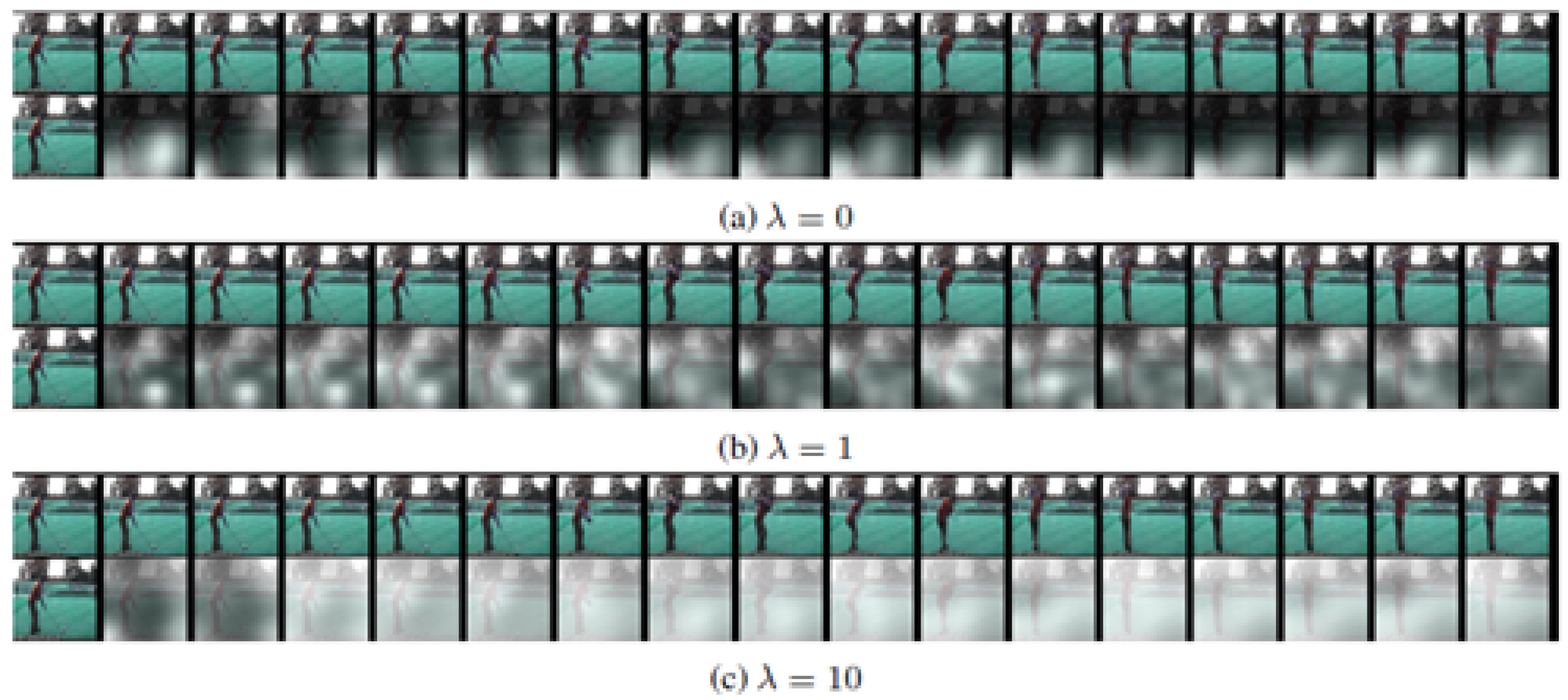
3.1.3. Loss Function and Attention Penalty

We use cross-entropy loss coupled with the doubly stochastic penalty introduced in Xu et al. [17]. We impose an additional constraint over the location softmax, so that ${\sum }_{t=1}^T{l}_{t,i}\approx 1$. This is the attention regularization which forces the model to look at each region of the frame at some point in time. The loss function is defined as follows:

$$L=-{\mathsf{\Sigma }}_{t=1}^T{\mathsf{\Sigma }}_{i=1}^C{y}_{t,i}log{\widehat{y}}_{t,i}+\lambda {\mathsf{\Sigma }}_{i=1}^{K^2}{(1-{\mathsf{\Sigma }}_{t=1^T{l}_{t,i}})}^2+\gamma {\mathsf{\Sigma }}_i{\mathsf{\Sigma }}_j{\theta }_{i,j}^2,$$

(12)

where $y_{t,i}$ is the i one hot label vector in time step t, ${\widehat{y}}_{t,i}$ is the i class probability vector in time step t, T is the total number of time steps, C is the number of output classes, $\lambda$ is the number of attention penalty coefficient, and $\gamma$ is the weight adjustment. And $\theta$ represents all model parameters of the $i,j$.

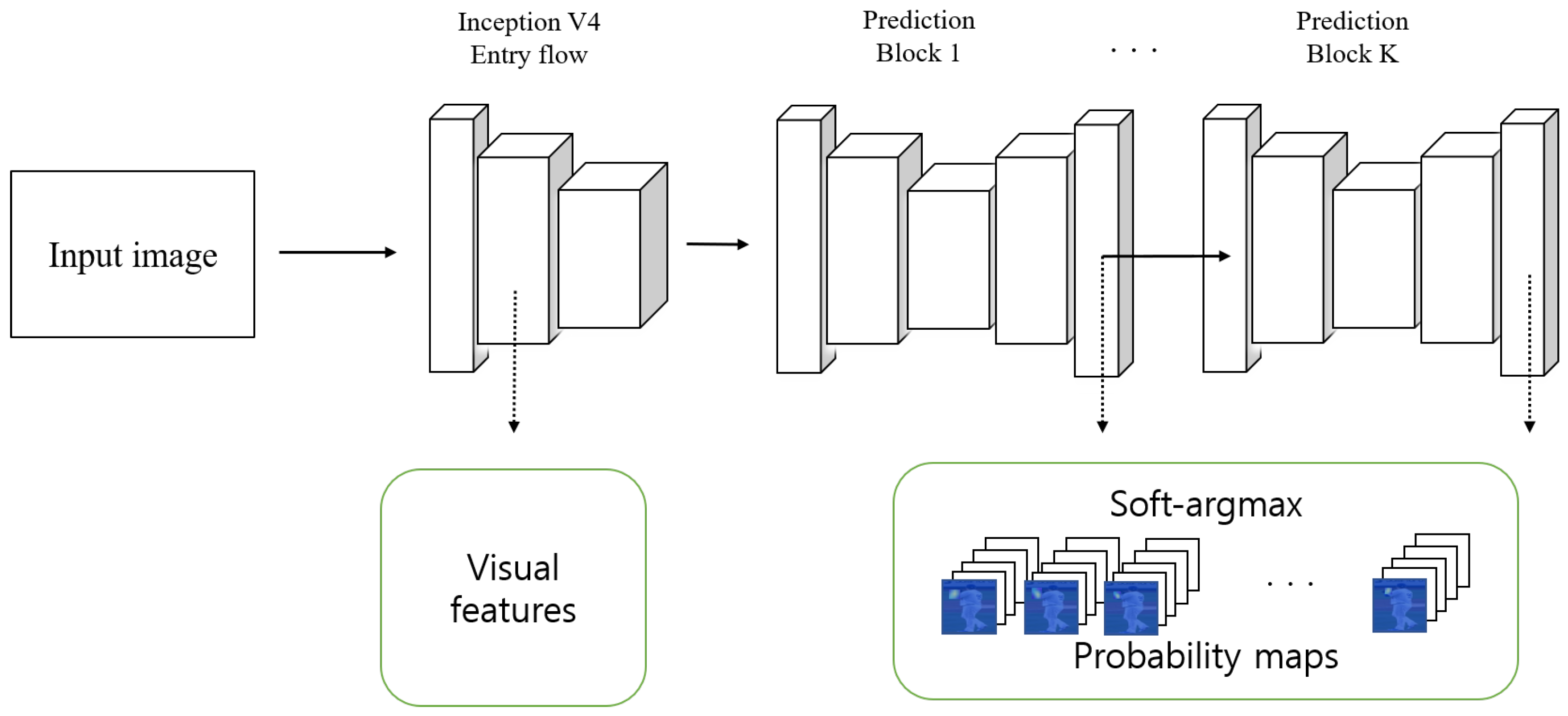
3.2. Pose Estimation

3.2.1. 3D Pose Estimation and Data Alignment

Recent development in deep learning has enabled hierarchical systems to learn powerful filters from data [42]. Furthermore, filters that are learned from large datasets can effectively be used for problems with insufficient data, using what is called transfer learning. The VNect approach propose in [43] is one of the systems that use transfer learning for effective 3D pose estimation directly from RGB images. VNect is based on a CNN pose regression that allows the real-time estimation of 2D and 3D skeletons using RGB image. For each estimated human joint, the network is trained to estimate a 2D confidence heatmap along with locations maps (for each of the three dimensions). One of the main advantages of estimating a 3D pose is the ability to estimate the positions of corresponding 3D points in different viewpoints. In which case, 3D pose alignment can be estimated with a closed-form solution. To further explain, let $x_1$ and $x_2$ be the estimates of the same subject’s 3D pose from two different viewpoints. Assuming the mean of the estimated pose is centered, the alignment of the estimated pose is performed by estimating the rotation R through the following optimization:

$$\underset{R}{argmin}{\parallel x_1-R{x}_2\parallel }_2^2$$

(13)

The Equation (13) has a closed-form solution given as

$$\tilde{R}=V{U}^T$$

(14)

where $U\sum V^T=x_1{x}_2^T$, with U and Vbeing unitary matrices and ∑ a diagonal matrix corresponding to the singular value decomposition (SVD) of $x_1{x}_2^T$. The matrix $\tilde{R}$ denotes the estimated rotation matrix. Given two sequences on n poses estimated from two different viewpoints $X_1=x_1^1,\cdots ,x_1^n$ and $X_2=x_2^1,\cdots ,x_2^n$, we estimate the alignment between the first corresponding poses $x_1^1$ and $x_2^1$ using Equation (14). Afterwards, the estimated rotation matrix R is used to align the rest of the subsequent poses of the sequence.

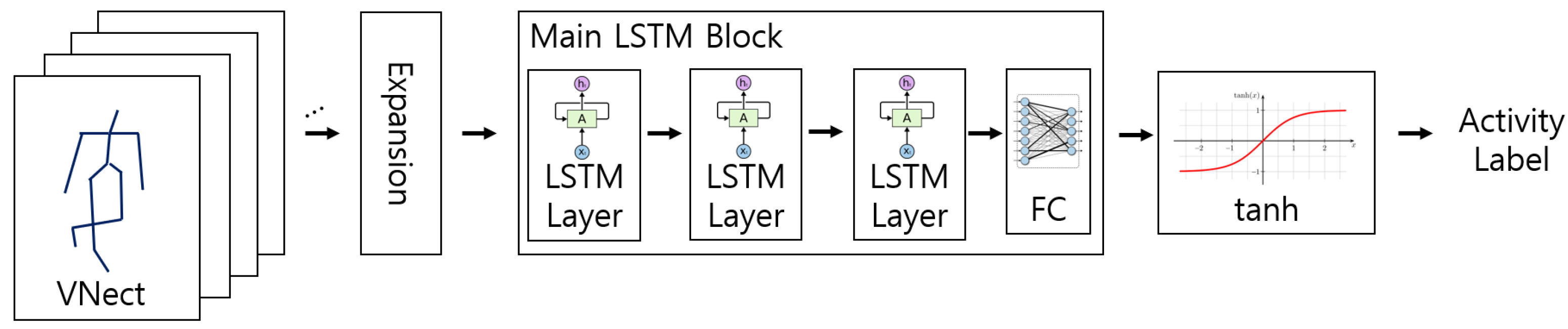
3.2.2. Pose Sequence Modelling

In general, 3D pose estimation from RGB data can be noisy depending on the estimation model and the available training dataset. In this subsection, we propose an LSTM-based temporal model that is suitable for estimating the temporal dependency between noisy skeletal pose estimates. Our approach has two main components: (1) a feed-forward network for expanding the data to a high-dimensional space, and (2) multi-layer LSTM units for modelling the temporal dependency. (see Figure 5) First, the description of data expansion. An estimated 3D skeleton with J number of joints is a vector in ${\mathbb{R}}^{3J}$. Hence, a noisy joint estimate is directly reflected on some of the dimensions of the observed vector. One typical solution for removing noise and redundancy is to contract the data to a lower dimensional space [44]. On the contrary, in this paper, we expand the data to a higher dimensional space. The main motivation for expanding the data is to disentangle explanatory factors that are obscured by noisy joint estimates. Consequently, the parameters of the expansion function are learned directly from the training dataset. Expansion of an observed skeleton is defined as follows:

$$\tilde{x}=tanh(Wx+b),$$

(15)

where W is a $k\times 3J$ matrix with $k\gg 3J$, b is a bias vector in a k-dimensional space, and the $\tilde{x}$ denotes the expanded pose estimate. Second, the description of temporal model and activity labeling. The temporal dependency between the sequential data points modelled using layers of LSTM units [6]. An LSTM is a gated recurrent neural network that models temporal dependency as a stationary process. While it has several components, we herein will refer to the integrated computational unit as LSTM. Subsequently, given an expanded input data $\tilde{x}$, we estimate hierarchical latent variables by layering LSTM units one on top of another, see Figure 5. Consequently, the inferred latent space from the i pose estimate is given as

$$h_i^L=LSTM\left({\tilde{x}}_i\right),$$

(16)

where L denotes the index of the last LSTM layer. Finally an activity label from a set $\mathsf{\Psi }$ is assigned to a sequence as

$$\tilde{\psi }=\underset{\psi \in \mathsf{\Psi }}{argmax}\left(tanh(W{h}_n^L+b)\right),$$

(17)

where n is the index of the last pose estimate. $\mathsf{\Psi }$ is the set of activity labels, $\psi$ is the activity label that can be output as a result, and $\tilde{\psi }$ is the final determined activity label. The connection weights and biases of the overall network (temporal model and data expansion) are trained together by minimizing the cross-entropy between the predicted and the given probability of an activity label via back-propagation and back-propagation through time [42]. In Figure 6, you can see that each joint represents a human skeleton. This uses VNect, and if the pose estimation result and the RGB-based result are combined as a result, the accuracy of similar motions that could not be properly classified is improved.

3.3. Activity Recognition

In Figure 7, visual features and probability maps are extracted using Inception V4. Visual features are extracted from the first network, and probability maps corresponding to each of the prediction blocks up to the K are extracted. Using the extracted visual features and probability maps, they are combined as shown in Figure 7 to create an appearance-based feature. Activity recognition is called appearance based recognition. The appearance based part is similar to the pose based part, with the difference that it relies on local appearance features instead of joint coordinates. In order to extract localized appearance features, we multiply the tensor of visual features $F_t\in {\mathbb{R}}^{W_f\times H_f\times N_f}$ obtained at the end of the global entry flow by the probability maps $M_t\in {\mathbb{R}}^{W_f\times H_f\times N_J}$ obtained at the end of the pose estimation part, where $W_f\times H_f$ is the size of the feature maps, $N_f$ is the number of features, and $N_J$ is the number of joints. Instead of multiplying each value individually as in the Kronecker product, we multiply each channel, resulting in a tensor of size ${\mathbb{R}}^{W_f\times H_f\times N_J\times N_f}$. Then, the spacial dimensions are collapsed by a sum, resulting in the appearance features for time t of size ${\mathbb{R}}^{N_J\times N_f}$. For a sequence of frames, we concatenate each appearance features for $t=0,1,...,T$ resulting in the video clip appearance features $V\in {\mathbb{R}}^{T\times N_J\times N_f}$. To clarify the above appearance features extraction process, a graphical representation is shown on Figure 8. Appearance features extraction from low level visual features and body parts probability maps for a single frame. For a sequence of T frames, the appearance features are stacked vertically producing a tensor where each line corresponds to one input frame.

4. Experiments

In this paper, the experiment was conducted after learning visual attention, activity recognition, and pose estimation with each data. UCF-11 [45], HMDB-51 [46], and Hollywood2 [47] datasets were used as a dataset for activity recognition using visual attention, NW-UCLA [48] as a dataset for pose estimation, and Penn Action [49], NTU RGB+D [50] as a dataset for activity recognition through appearance. The experiment was carried out using.

4.1. Datasets

UCF-11 is a Youtube Action dataset consisting of 11 activities such as basketball shooting, cycling, diving, golf swing, horseback riding, soccer, juggling, tennis, trampoline, volleyball and walking. The clip has a frame rate of 29.97 FPS (Frames Per Second), and each video has only one linked activity. We use 975 videos for training and 625 videos for testing. The HMDB-51 Human Motion Database data set provides 3 training data consisting of 5100 videos each. There are 51 kinds of human activities in this clip, such as clapping, drinking, hugging, jumping, and throwing. There are 3570 videos in the training set and 1530 videos in the test set. The frame rate of the clip is 30 FPS. The Hollywood2 Human Actions data set consists of 1707 video clips collected from movies. There are 12 types of human behavior in this clip: driving, eating, fighting, shaking hands, hugging, kissing, running, standing up, sitting, and answering the phone. There are 823 videos in the training set and 884 videos in the test set. All videos in the dataset were scaled to resolution and provided to a GoogLeNet model trained on the ImageNet dataset. The last convolutional layer of $7\times 7\times 1024$ was used as input to the model. The NW-UCLA data set is one of the RGB-D based data sets. It consists of 1494 videos in 10 activity classes: pick up with one hand, pick up with two hands, throw away trash, walk, sit down, stand up, put on, take off, throw, and move. Each activity was performed 1–6 times per learning. The data set is provided with RGB and depth corresponding expected 3D skeleton sequences. For the experiment, the segmentation protocol proposed by Wang et al. [51] is followed. The Penn Action data set consists of 2326 videos containing 15 activities including baseball pitching, bench press, and guitar striking. The disadvantage of this data set was that several body parts were missing from many tasks and the image scale was different from sample to sample. The NTU RGB+D data set is a data set for 3D activity recognition. It consists of a Full HD 56 K video of 60 activities performed by 40 actors, and is recorded with 3 cameras at 17 different position settings, providing over 4 M video frames.

4.2. Experimental Environment and Parameter Setting

In experiments for visual attention, the model architecture and various other hyperparameters were set using cross validation. Specifically, we trained with a 3-layer LSTM model with dimensions of the LSTM hidden state, cell state, and hidden layer set to 512 for UCF-11 and Hollywood2 and 1024 for HMDB-51 for all data sets. We also tested a model with 5 LSTM layers in 1 LSTM layer, but the model performance did not improve significantly. The attention penalty coefficients were tested with 0, 1, and 10 values. Drop out was used as 0.5. All models are based on the method proposed by Bastien et al. [52] for the entire data set and also handle slope calculation. For both training and testing, the model in this paper uses 30 frames sampled at a fixed FPS rate. Each video is divided into groups of 30 frames starting from the first frame, selecting 30 frames according to the FPS rate, and then proceeding to stride 1. Thus, each video is divided into several 30 length samples. At test time, class predictions for each time step are computed and these predictions are averaged over 30 frames. The predictions are averaged over all 30 frame blocks of the video to get a prediction for the entire video clip. In Figure 9, changes of attention penalty are shown with varying $\lambda$.

The Softmax regression model uses $7\times 7\times 1024$ feature cubes as inputs to predict labels at each time step, while all other models only use 1024 dimensional feature slices as inputs. In Figure 10, you can see the change in visual attention according to the visual attention penalty $\lambda$ value. If $\lambda$ values are 1 or 10, it is difficult to say that a proper weight value is calculated because it gives a visual attention effect to too many parts. However, when the value is set to 0, the hyperparameter value is set to 0 because the person attends on the part where they play golf and attends their visuals.

In Figure 10, playing soccer and playing golf were accurately recognized. However, the figure below shows that he is playing golf but is jumping, or he is doing squat but is playing hugs. You can see that the part marked in white is inaccurately attending on the visual. In this way, when only the visual attention algorithm is used, it may not be accurately found. To solve this problem, pose estimation, activity recognition, and visual attention are all necessary. For pose estimation, we used a pre-trained VNect model that provides a 3D joint estimate with 20 joints per frame to estimate a 3D joint sequence from an RGB video provided by NW-UCLA. In addition, the joint sequences were temporally aligned using zero padding in an automated manner. In the experiment, the batch size was set to 2 considering the small size of the NW-UCLA dataset. Also, using cross-validation, the optimal learning rate was set to 0.0002 and the number of epochs was selected as 100. The architecture implementation is based on PyTorch, which uses 128 hidden units per layer. For appearance-based activity recognition, Penn Action and NTU RGB+D datasets are used. When training, we train the network using the cross entropy loss, and at training we randomly select a fixed size clip with T frames from the video samples. Use the results for a single clip or multiple clips in the test. In the first case, you cut a single clip in the middle of the video. In the second case, we cut out several clips at $T/2$ frame intervals in time. The final score for multiple clips is calculated as the average result for all clips in a video. To estimate the bounding box in the test, the prediction is performed using the entire image of the first, middle, and last frame of the clip.

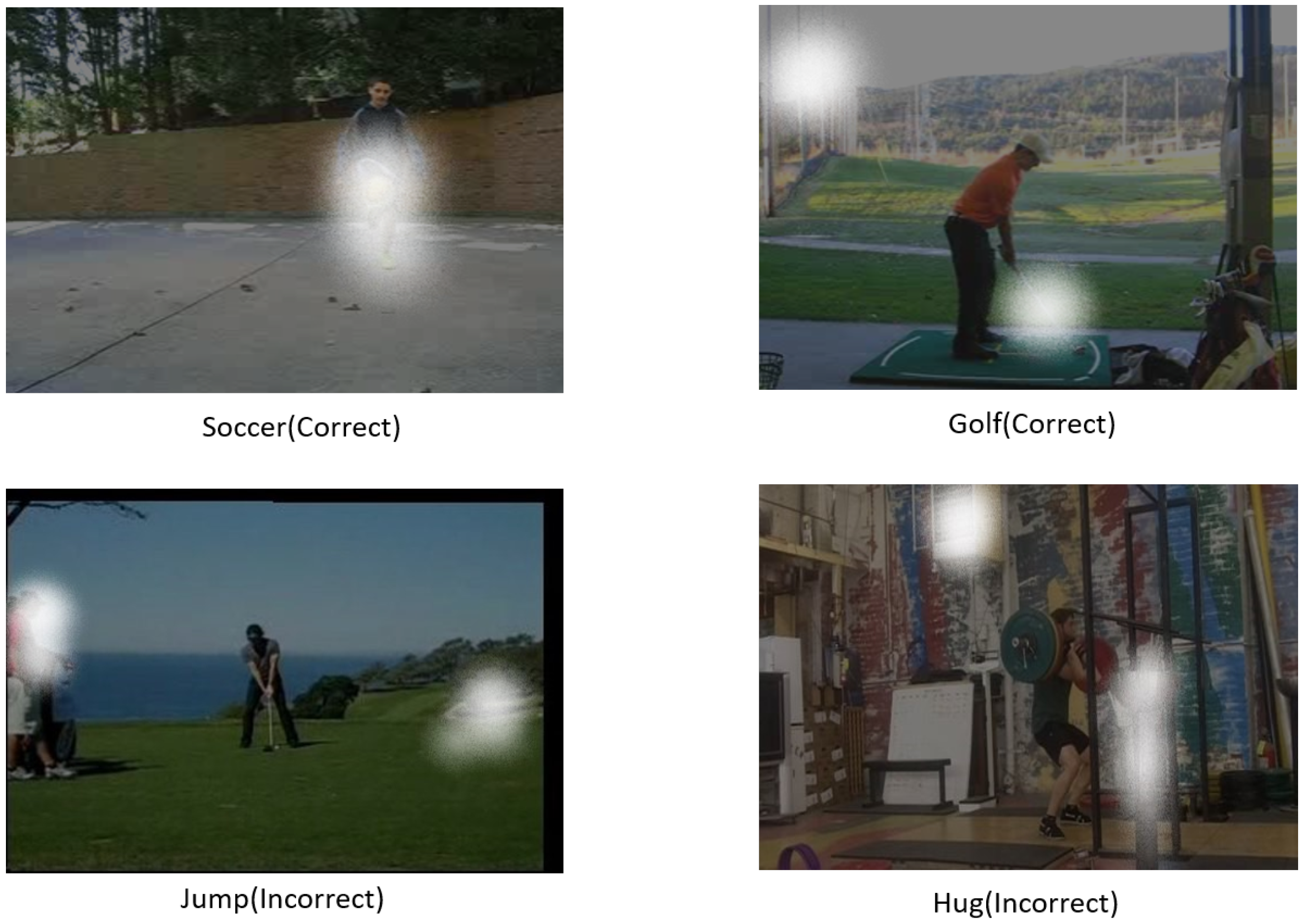
4.3. Experiment Result

Table 2. Experimental results with the Penn Action dataset.

Methods	RGB	Optical Flow	Estimated Poses	Visual Attention	Accuracy
Nie et al. [21]	X	O	X	X	85.5%
Iqbal et al. [53]	O	O	X	X	79.0%
Iqbal et al. [53]	X	X	X	X	92.9%
Cao et al. [22]	X	O	O	X	98.1%
Cao et al. [22]	X	O	X	X	95.3%
Based on Visual attention	O	O	X	O	97.7%
Based on Estimated poses	O	O	O	X	97.9%
Proposed	O	O	O	O	98.9%

shows the experimental results using the Penn Action dataset. Each experiment was performed using different input data. Basically, appearance-based data was used as input, and the accuracy of the final activity recognition was calculated when the pose estimation result was added, the visual attention result was added, and the pose estimation result and the visual attention result were added. When only the pose estimation result was added, it was 97.9%, when only the visual attention resultwas added, it was 97.7%, and when both were added, it was 98.9%, which was 0.8% higher than theresult suggested by Cao et al. [22].

Table 3. Experimental results with the NTU dataset.

Methods	Kinect Poses	RGB	Estimated Poses	Visual Attention	Accuracy
Shahroudy et al. [54]	X	O	O	X	62.9%
Liu et al. [25]	X	O	O	X	69.2%
Song et al. [55]	X	O	O	X	73.4%
Liu et al. [26]	X	O	O	X	74.4%
Shahroudy et al. [56]	X	X	O	X	74.9%
Baradel et al. [27]	X	O	O	X	77.1%
Baradel et al. [27]	O	X	O	X	75.6%
Baradel et al. [27]	X	X	O	X	84.8%
Based on Visual attention	X	O	X	O	87.5%
Based on Estimated poses	X	O	O	X	87.7%
Proposed	X	O	O	O	87.9%

shows the experimental results using the NTU dataset. Since NTU’s skeletal data is often noisy, we trained with 10% of the NTU’s data and 90% of the pose estimation data using video clips of 20 body joints and frames. As shown in Table 2, the method in this paper improves accuracy by adding RGB frames, pose estimation, and visual attention results. It is 87.7% when only RGB frame and pose estimation are added, 87.5% when only visual attention is added, and 87.9% when both are added, which is 25% better than the method proposed by Shahroudy et al. [54]. Many of the previous methods use the posture provided by Kinect-v2. This pose estimation result is known to be noisy. As shown in Table 3, the method of this paper improves accuracy by 12.3% compared to the method proposed by Baradel et al. [27] using Kinect when pose estimation is added. This means that the performance is better when visual attention is used than when visual attention is not used. And the performance is better when the pose estimation is added than when it is not added. In addition, there may be limitations with only one method of visual attention, pose estimation, and appearance-based activity recognition, but it can be said that the accuracy was improved by complementing the limitations.

Table 4. Experimental results with the NW-UCLA dataset.

Methods	Accuracy
No expansion + LSTM	79.9
Expansion + LSTM	83.4
VNect + Expansion + LSTM	87.2
Proposed	88.6

shows the results of experiments on the NW-UCLA dataset. First, the accuracy improved to 79.9% when only the extension and LSTM were used, and 83.4% when only the extension and LSTM were used. In addition, when VNect is used, it is 87.2%, which is improved by 3.8%, and when the method proposed in this paper is used, it shows the highest performance at 88.6%. Figure 11 shows the results of loss function value during training.

5. Conclusions

In this paper, we proposed activity recognition that considers visual attention, pose estimation, and activity recognition. Through the visual attention algorithm, weights are added to the necessary parts to enable attention calculation. The visual attention algorithm uses a soft visual attention algorithm to enable calculation without increasing the amount of calculation. And we use VNect to estimate the pose. If only appearance-based activity recognition is used, it is not possible to accurately distinguish between similar activities. However, if you have information about pose estimation, it is possible to accurately recognize similar activities due to different joints. It performs appearance-based activity recognition with information on visual attention and activity recognition. For this reason, the information of all three is synthesized to estimate the final activity recognition label. UFC-11, HMDB-51, and Hollywood2 datasets were used for visual attention, and NW-UCLA was used as activity recognition dataset through pose estimation. And Penn Action, NTU RGB+D was used as a data set for appearance-based activity recognition. Intel${}^{\circledR }$ Core™ i3-8100 CPU @ 3.60 GHz was used as the experiment environment, and Geforce 2070 RTX was used as the GPU. In addition, 24 GB of RAM is used, and the experiment was conducted on the operating system of Ubuntu 16.04. Existing appearance estimation-based activity recognition algorithms show 98.9% accuracy for the Penn Action dataset, 87.9% for the NTU dataset, and 88.6% for the NW-UCLA dataset. The advantage of such an algorithm is that it is possible to accurately recognize activities with a lot of information even for parts that cannot be accurately identified. However, despite the use of the soft visual attention algorithm, an increase in the amount of computation is inevitable in order to perform all three. Therefore, it is not suitable for use in real-time activity recognition estimation. In order to improve these pinkshortcomings, it is necessary to devise a method that does not increase the amount of calculation but can maintain or improve the accuracy. If the accuracy is improved without increasing theamount of calculation, it can be applied in fields requiring real-time processing. In addition, a detailed analysis of each class is required. While there are classes with improved accuracy such as drinking water and answering calls, there are classes with no improved accuracy, such as walking and playing basketball. Therefore, by analyzing the class with improved accuracy and the class with no improved accuracy, we will devise a method to improve the accuracy even in the class with no improved accuracy. In conclusion, we proposed an activity recognition method that considers visual attention, pose estimation, and activity recognition, and we plan to research a method to improve accuracy and reduce the amount of computation as a future work.

References

1. Chéron, G.; Laptev, I.; Schmid, C. P-cnn: Pose-based cnn features for action recognition. In Proceedings of the IEEE International Conference on Computer Vision, Santiago, Chile, 7–13 December 2015; pp. 3218–3226. [Google Scholar]
2. Kokkinos, I. Ubernet: Training a universal convolutional neural network for low-, mid-, and high-level vision using diverse datasets and limited memory. In Proceedings of the IEEE Conference on Computer Vision and Pattern Recognition, Honolulu, HI, USA, 21–26 July 2017; pp. 6129–6138. [Google Scholar]
3. Newell, A.; Yang, K.; Deng, J. Stacked hourglass networks for human pose estimation. In Proceedings of the European Conference on Computer Vision, Amsterdam, The Netherlands, 11–14 October 2016; pp. 483–499. [Google Scholar]
4. Baradel, F.; Wolf, C.; Mille, J. Human action recognition: Pose-based attention draws focus to hands. In Proceedings of the IEEE International Conference on Computer Vision Workshops, Venice, Italy, 22–29 October 2017; pp. 604–613. [Google Scholar]
5. Rensink, R.A. The dynamic representation of scenes. Vis. Cogn. 2000, 7, 17–42. [Google Scholar] [CrossRef]
6. Schmidhuber, J.; Hochreiter, S. Long short-term memory. Neural Comput. 1997, 9, 1735–1780. [Google Scholar]
7. Williams, R.J. Simple statistical gradient-following algorithms for connectionist reinforcement learning. Mach. Learn. 1992, 8, 229–256. [Google Scholar] [CrossRef] [Green Version]
8. Wang, J.; Hafidh, B.; Dong, H.; El Saddik, A. Sitting Posture Recognition Using a Spiking Neural Network. IEEE Sens. J. 2020, 21, 1779–1786. [Google Scholar] [CrossRef]
9. Nadeem, A.; Jalal, A.; Kim, K. Automatic human posture estimation for sport activity recognition with robust body parts detection and entropy markov model. Multimed. Tools Appl. 2021, 1–34. [Google Scholar] [CrossRef]
10. Kulikajevas, A.; Maskeliunas, R.; Damaševičius, R. Detection of sitting posture using hierarchical image composition and deep learning. PeerJ Comput. Sci. 2021, 7, e442. [Google Scholar] [CrossRef]
11. Ren, S.; He, K.; Girshick, R.; Zhang, X.; Sun, J. Object detection networks on convolutional feature maps. IEEE Trans. Pattern Anal. Mach. Intell. 2016, 39, 1476–1481. [Google Scholar] [CrossRef] [PubMed] [Green Version]
12. Wu, R.; Yan, S.; Shan, Y.; Dang, Q.; Sun, G. Deep image: Scaling up image recognition. arXiv 2015, arXiv:1501.02876. [Google Scholar]
13. Graves, A.; Jaitly, N.; Mohamed, A.R. Hybrid speech recognition with deep bidirectional LSTM. In Proceedings of the 2013 IEEE Workshop on Automatic Speech Recognition and Understanding, Olomouc, Czech Republic, 8–13 December 2013; pp. 273–278. [Google Scholar]
14. Yao, L.; Torabi, A.; Cho, K.; Ballas, N.; Pal, C.; Larochelle, H.; Courville, A. Describing videos by exploiting temporal structure. In Proceedings of the IEEE International Conference on Computer Vision, Santiago, Chile, 7–13 December 2015; pp. 4507–4515. [Google Scholar]
15. Srivastava, N.; Mansimov, E.; Salakhudinov, R. Unsupervised learning of video representations using lstms. In Proceedings of the International Conference on Machine Learning, Lille, France, 6–11 July 2015; pp. 843–852. [Google Scholar]
16. Karpathy, A.; Toderici, G.; Shetty, S.; Leung, T.; Sukthankar, R.; Fei-Fei, L. Large-scale video classification with convolutional neural networks. In Proceedings of the IEEE conference on Computer Vision and Pattern Recognition, Columbus, OH, USA, 23–28 June 2014; pp. 1725–1732. [Google Scholar]
17. Xu, K.; Ba, J.; Kiros, R.; Cho, K.; Courville, A.; Salakhudinov, R.; Zemel, R.; Bengio, Y. Show, attend and tell: Neural image caption generation with visual attention. In Proceedings of the International Conference on Machine Learning, Lille, France, 6–11 July 2015; pp. 2048–2057. [Google Scholar]
18. Jaderberg, M.; Simonyan, K.; Zisserman, A.; Kavukcuoglu, K. Spatial transformer networks. In Proceedings of the Advances in Neural Information Processing Systems, Montreal, QC, Canada, 7–12 December 2015; pp. 2017–2025. [Google Scholar]
19. Netzer, Y.; Wang, T.; Coates, A.; Bissacco, A.; Wu, B.; Ng, A.Y. Reading Digits in Natural Images with Unsupervised Feature Learning. 2011. Available online: https://api.semanticscholar.org/CorpusID:16852518 (accessed on 6 December 2020).
20. Yeung, S.; Russakovsky, O.; Jin, N.; Andriluka, M.; Mori, G.; Fei-Fei, L. Every moment counts: Dense detailed labeling of actions in complex videos. Int. J. Comput. Vis. 2018, 126, 375–389. [Google Scholar] [CrossRef] [Green Version]
21. Xiaohan Nie, B.; Xiong, C.; Zhu, S.C. Joint action recognition and pose estimation from video. In Proceedings of the IEEE Conference on Computer Vision and Pattern Recognition, Boston, MA, USA, 7–12 June 2015; pp. 1293–1301. [Google Scholar]
22. Cao, C.; Zhang, Y.; Zhang, C.; Lu, H. Body joint guided 3-d deep convolutional descriptors for action recognition. IEEE Trans. Cybern. 2017, 48, 1095–1108. [Google Scholar] [CrossRef] [PubMed] [Green Version]
23. Baradel, F.; Wolf, C.; Mille, J.; Taylor, G.W. Glimpse clouds: Human activity recognition from unstructured feature points. In Proceedings of the IEEE Conference on Computer Vision and Pattern Recognition, Salt Lake City, UT, USA, 18–23 June 2018; pp. 469–478. [Google Scholar]
24. Luvizon, D.C.; Tabia, H.; Picard, D. Learning features combination for human action recognition from skeleton sequences. Pattern Recognit. Lett. 2017, 99, 13–20. [Google Scholar] [CrossRef] [Green Version]
25. Liu, J.; Shahroudy, A.; Xu, D.; Wang, G. Spatio-temporal lstm with trust gates for 3d human action recognition. In Proceedings of the European Conference on Computer Vision, Amsterdam, The Netherlands, 11–14 October 2016; pp. 816–833. [Google Scholar]
26. Liu, J.; Wang, G.; Hu, P.; Duan, L.Y.; Kot, A.C. Global context-aware attention lstm networks for 3d action recognition. In Proceedings of the IEEE Conference on Computer Vision and Pattern Recognition, Honolulu, HI, USA, 21–26 July 2017; pp. 1647–1656. [Google Scholar]
27. Baradel, F.; Wolf, C.; Mille, J. Pose-conditioned spatio-temporal attention for human action recognition. arXiv 2017, arXiv:1703.10106. [Google Scholar]
28. Andriluka, M.; Roth, S.; Schiele, B. Pictorial structures revisited: People detection and articulated pose estimation. In Proceedings of the 2009 IEEE Conference on Computer Vision and Pattern Recognition, Miami, FL, USA, 20–25 June 2009; pp. 1014–1021. [Google Scholar]
29. Ning, G.; Zhang, Z.; He, Z. Knowledge-guided deep fractal neural networks for human pose estimation. IEEE Trans. Multimed. 2017, 20, 1246–1259. [Google Scholar] [CrossRef]
30. Bulat, A.; Tzimiropoulos, G. Human pose estimation via convolutional part heatmap regression. In Proceedings of the European Conference on Computer Vision, Amsterdam, The Netherlands, 11–14 October 2016; pp. 717–732. [Google Scholar]
31. Yang, W.; Li, S.; Ouyang, W.; Li, H.; Wang, X. Learning feature pyramids for human pose estimation. In Proceedings of the IEEE International Conference on Computer Vision, Venice, Italy, 22–29 October 2017; pp. 1281–1290. [Google Scholar]
32. Chen, Y.; Shen, C.; Wei, X.S.; Liu, L.; Yang, J. Adversarial posenet: A structure-aware convolutional network for human pose estimation. In Proceedings of the IEEE International Conference on Computer Vision, Venice, Italy, 22–29 October 2017; pp. 1212–1221. [Google Scholar]
33. Toshev, A.; Szegedy, C. Deeppose: Human pose estimation via deep neural networks. In Proceedings of the IEEE Conference on Computer Vision And Pattern Recognition, Columbus, OH, USA, 23–28 June 2014; pp. 1653–1660. [Google Scholar]
34. Carreira, J.; Agrawal, P.; Fragkiadaki, K.; Malik, J. Human pose estimation with iterative error feedback. In Proceedings of the IEEE Conference on Computer Vision And Pattern Recognition, Las Vegas, NV, USA, 27–30 June 2016; pp. 4733–4742. [Google Scholar]
35. Luvizon, D.C.; Tabia, H.; Picard, D. Human pose regression by combining indirect part detection and contextual information. Comput. Graph. 2019, 85, 15–22. [Google Scholar] [CrossRef] [Green Version]
36. Ionescu, C.; Papava, D.; Olaru, V.; Sminchisescu, C. Human3. 6m: Large scale datasets and predictive methods for 3d human sensing in natural environments. IEEE Trans. Pattern Anal. Mach. Intell. 2013, 36, 1325–1339. [Google Scholar] [CrossRef] [PubMed]
37. Zhou, X.; Zhu, M.; Pavlakos, G.; Leonardos, S.; Derpanis, K.G.; Daniilidis, K. Monocap: Monocular human motion capture using a cnn coupled with a geometric prior. IEEE Trans. Pattern Anal. Mach. Intell. 2018, 41, 901–914. [Google Scholar] [CrossRef] [PubMed] [Green Version]
38. Sun, X.; Shang, J.; Liang, S.; Wei, Y. Compositional human pose regression. In Proceedings of the IEEE International Conference on Computer Vision, Venice, Italy, 22–29 October 2017; pp. 2602–2611. [Google Scholar]
39. Pavlakos, G.; Zhou, X.; Derpanis, K.G.; Daniilidis, K. Coarse-to-fine volumetric prediction for single-image 3D human pose. In Proceedings of the IEEE Conference on Computer Vision and Pattern Recognition, Honolulu, HI, USA, 21–26 July 2017; pp. 7025–7034. [Google Scholar]
40. Deng, J.; Dong, W.; Socher, R.; Li, L.J.; Li, K.; Li, F.-F. Imagenet: A large-scale hierarchical image database. In Proceedings of the 2009 IEEE Conference on Computer Vision and Pattern Recognition, Miami, FL, USA, 20–25 June 2009; pp. 248–255. [Google Scholar]
41. Szegedy, C.; Liu, W.; Jia, Y.; Sermanet, P.; Reed, S.; Anguelov, D.; Erhan, D.; Vanhoucke, V.; Rabinovich, A. Going deeper with convolutions. In Proceedings of the IEEE Conference on Computer Vision And Pattern Recognition, Boston, MA, USA, 7–12 June 2015; pp. 1–9. [Google Scholar]
42. Goodfellow, I.; Bengio, Y.; Courville, A.; Bengio, Y. Deep Learning; MIT Press: Cambridge, MA, USA, 2016; Volume 1. [Google Scholar]
43. Mehta, D.; Sridhar, S.; Sotnychenko, O.; Rhodin, H.; Shafiei, M.; Seidel, H.P.; Xu, W.; Casas, D.; Theobalt, C. Vnect: Real-time 3d human pose estimation with a single rgb camera. ACM Trans. Graph. TOG 2017, 36, 1–14. [Google Scholar] [CrossRef] [Green Version]
44. Van Der Maaten, L.; Postma, E.; Van den Herik, J. Dimensionality reduction: A comparative. J. Mach. Learn. Res. 2009, 10, 13. [Google Scholar]
45. Liu, J.; Luo, J.; Shah, M. Recognizing realistic actions from videos “in the wild”. In Proceedings of the 2009 IEEE Conference on Computer Vision and Pattern Recognition, Miami, FL, USA, 22–24 June 2009; pp. 1996–2003. [Google Scholar]
46. Kuehne, H.; Jhuang, H.; Garrote, E.; Poggio, T.; Serre, T. HMDB: A large video database for human motion recognition. In Proceedings of the 2011 International Conference on Computer Vision, Barcelona, Spain, 6–13 November 2011; pp. 2556–2563. [Google Scholar]
47. Marszalek, M.; Laptev, I.; Schmid, C. Actions in context. In Proceedings of the 2009 IEEE Conference on Computer Vision and Pattern Recognition, Miami, FL, USA, 20–25 June 2009; pp. 2929–2936. [Google Scholar]
48. Zhang, J.; Li, W.; Ogunbona, P.O.; Wang, P.; Tang, C. RGB-D-based action recognition datasets: A survey. Pattern Recognit. 2016, 60, 86–105. [Google Scholar] [CrossRef] [Green Version]
49. Zhang, W.; Zhu, M.; Derpanis, K.G. From actemes to action: A strongly-supervised representation for detailed action understanding. In Proceedings of the IEEE International Conference on Computer Vision, Sydney, Australia, 1–8 December 2013; pp. 2248–2255. [Google Scholar]
50. Sedmidubsky, J.; Elias, P.; Zezula, P. Benchmarking Search and Annotation in Continuous Human Skeleton Sequences. In Proceedings of the 2019 on International Conference on Multimedia Retrieval, Ottawa, ON, Canada, 10–13 June 2019; pp. 38–42. [Google Scholar]
51. Wang, J.; Nie, X.; Xia, Y.; Wu, Y.; Zhu, S.C. Cross-view action modeling, learning and recognition. In Proceedings of the IEEE Conference on Computer Vision and Pattern Recognition, Columbus, OH, USA, 23–28 June 2014; pp. 2649–2656. [Google Scholar]
52. Bastien, F.; Lamblin, P.; Pascanu, R.; Bergstra, J.; Goodfellow, I.; Bergeron, A.; Bouchard, N.; Warde-Farley, D.; Bengio, Y. Theano: New features and speed improvements. arXiv 2012, arXiv:1211.5590. [Google Scholar]
53. Iqbal, U.; Garbade, M.; Gall, J. Pose for action-action for pose. In Proceedings of the 2017 12th IEEE International Conference on Automatic Face & Gesture Recognition (FG 2017), Washington, DC, USA, 30 May–3 June 2017; pp. 438–445. [Google Scholar]
54. Shahroudy, A.; Liu, J.; Ng, T.T.; Wang, G. Ntu rgb+ d: A large scale dataset for 3d human activity analysis. In Proceedings of the IEEE Conference on Computer Vision And Pattern Recognition, Las Vegas, NV, USA, 27–30 June 2016; pp. 1010–1019. [Google Scholar]
55. Song, S.; Lan, C.; Xing, J.; Zeng, W.; Liu, J. An end-to-end spatio-temporal attention model for human action recognition from skeleton data. arXiv 2016, arXiv:1611.06067. [Google Scholar]
56. Shahroudy, A.; Ng, T.T.; Gong, Y.; Wang, G. Deep multimodal feature analysis for action recognition in rgb+ d videos. IEEE Trans. Pattern Anal. Mach. Intell. 2017, 40, 1045–1058. [Google Scholar] [CrossRef] [PubMed] [Green Version]
Figure 1. Original image (top), image with visual attention applied (bottom). The area marked in white has a high attention weight.
Applsci 11 04153 g001
Figure 2. Overall structure of the proposed algorithm. Our method provides 2D/3D pose estimation from video frames. Pose, visual and appearance are used to predict activities in a unified framework.
Applsci 11 04153 g002
Figure 3. Our recurrent model. At each time-step t, our recurrent network takes a feature slice x t , generated as in Figure 4, as the input. It then propagates x t through three layers of LSTMs and predicts the next location probabilities I t + 1 and the class label y t .
Applsci 11 04153 g003
Figure 4. Soft attention mechanism. The CNN takes video frame as its input and produces a feature cube. The model computes the current input x t as an average of the feature slices weighted according to the location softmax I t .
Applsci 11 04153 g004
Figure 5. Proposed network for activity recognition using pose estimation. FC refers to the fully connected layer at the end of the main LSTM block.
Applsci 11 04153 g005
Figure 6. Result of pose estimation. Figure shows the skeletons for pitching, bench press, and bowling poses, respectively.
Applsci 11 04153 g006
Figure 7. Visual feature and probability map extraction algorithm through Inception V4. Human pose regression approach from a video frame. The input video is fed through a CNN composed by one entry flow and K prediction blocks. Predictions are refined at each prediction block.
Applsci 11 04153 g007
Figure 8. Appearance based activity recognition. Appearance features extraction from low level visual features and body parts probability maps for a single frame. For a sequence of T frames, the appearance features are stacked vertically producing a tensor where each line corresponds to one input frame.
Applsci 11 04153 g008
Figure 9. Attention penalty value changes in visual attention according to the λ value. The white regions are where the model is looking and the brightness indicates the strength of focus. Setting λ = 0 corresponds to the model that tends to select a few locations and stay fixed on them. Setting λ = 10 forces the model to gaze everywhere, which resembles average pooling over slices.
Applsci 11 04153 g009
Figure 10. Activity recognition results using visual attention. Soccer and Golf are paying attention correctly (Top). But Jump and Hug are wrong (Bottom).
Applsci 11 04153 g010
Figure 11. Loss function value during training.
Applsci 11 04153 g011