
A Novel MRA-Based Framework for Segmenting the Cerebrovascular System and Correlating Cerebral Vascular Changes to Mean Arterial Pressure

 , ,
, ,  ,
,  and
and 
Abstract
Featured Application
Abstract
1. Introduction
2. Materials and Methods
2.1. Patient Demographics
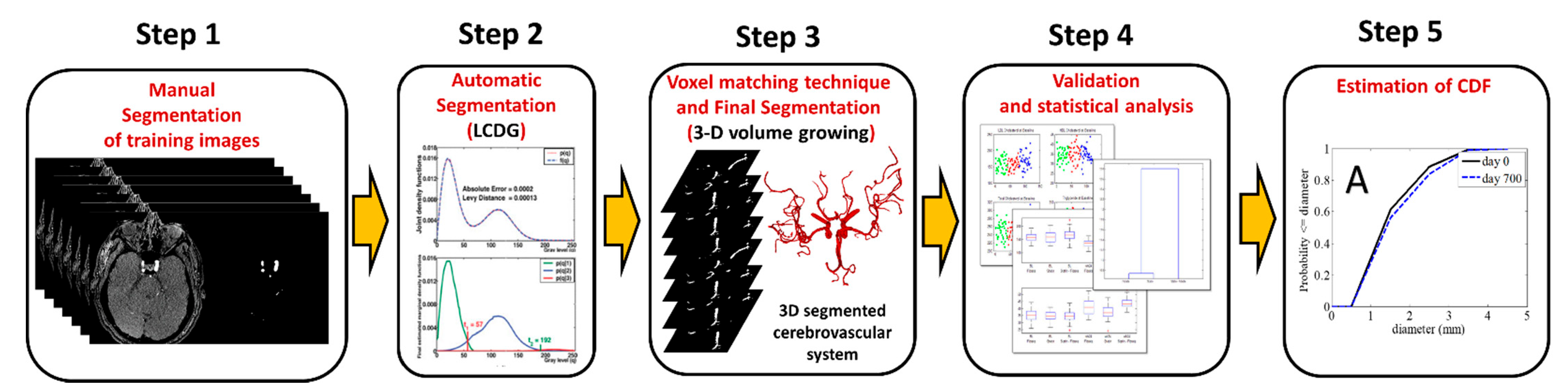
2.2. Data Analysis
- (1)
- For every slice Xs, s=1,…..S,
- (a)
- First is to gather the marginal empirical probability distribution Fs of gray levels.
- (b)
- Find a starting LCDG model which is nearing Fs by using the initialization algorithm to approximate the values of Cp−K, Cn, and the parameters w, Θ (weights, means, and variances) of the negative and positive discrete Gaussians (DG).
- (c)
- Fixing Cp and Cn, refine the LCDG-model with the modified EM algorithm by manipulating the other parameters.(See Appendix A for more details)
- (d)
- Separate the final LCDG model into K sub models. Each dominant mode has a corresponding sub model. This is done by minimizing the misclassification predicted errors and selecting the LCDG-sub model that has the greatest average value (corresponding to the pixels with highest brightness) to be the model of the wanted vasculature.
- (e)
- Use intensity threshold t to extract the voxels of the blood vessels in the MRA slice, which separates their LCDG-sub model from the background.
- (2)
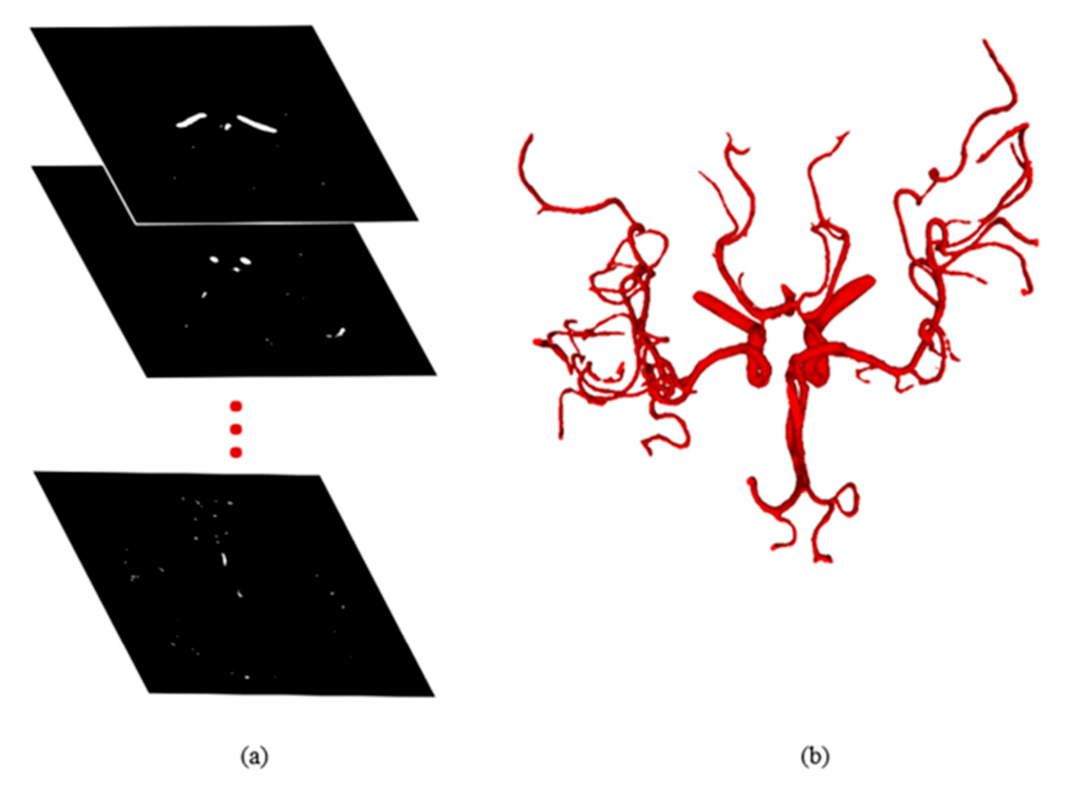
- Remove the artifacts from the extracted voxels whole set with a connection filter which chooses the greatest connected tree system built by a 3D growing algorithm [23]. Algorithm 1 summarizes the adopted segmentation approach.
| Algorithm 1. Segmentation Approach Main Steps. |
For every slice Xs, the following steps were completed:
|
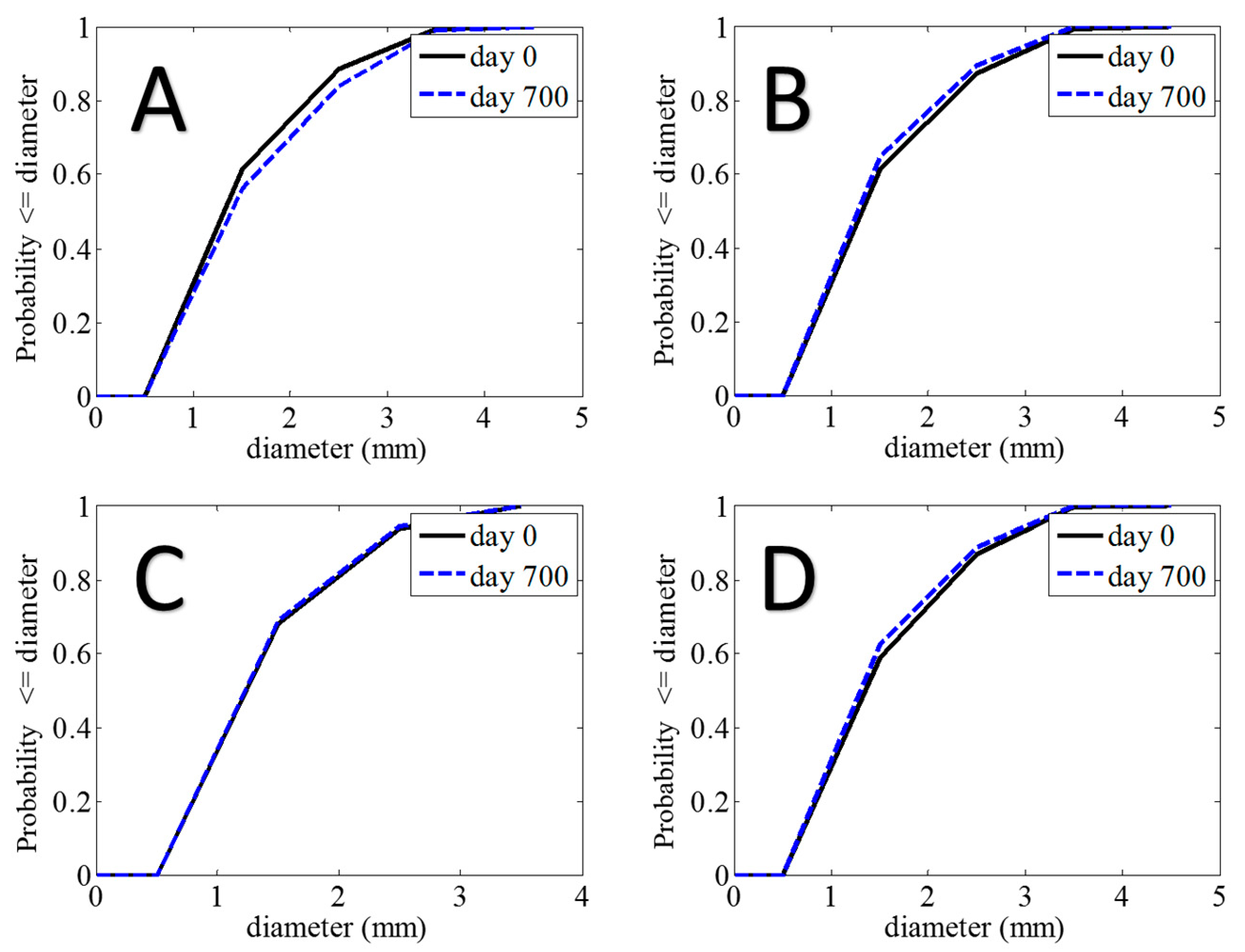
2.3. Statistical Analysis
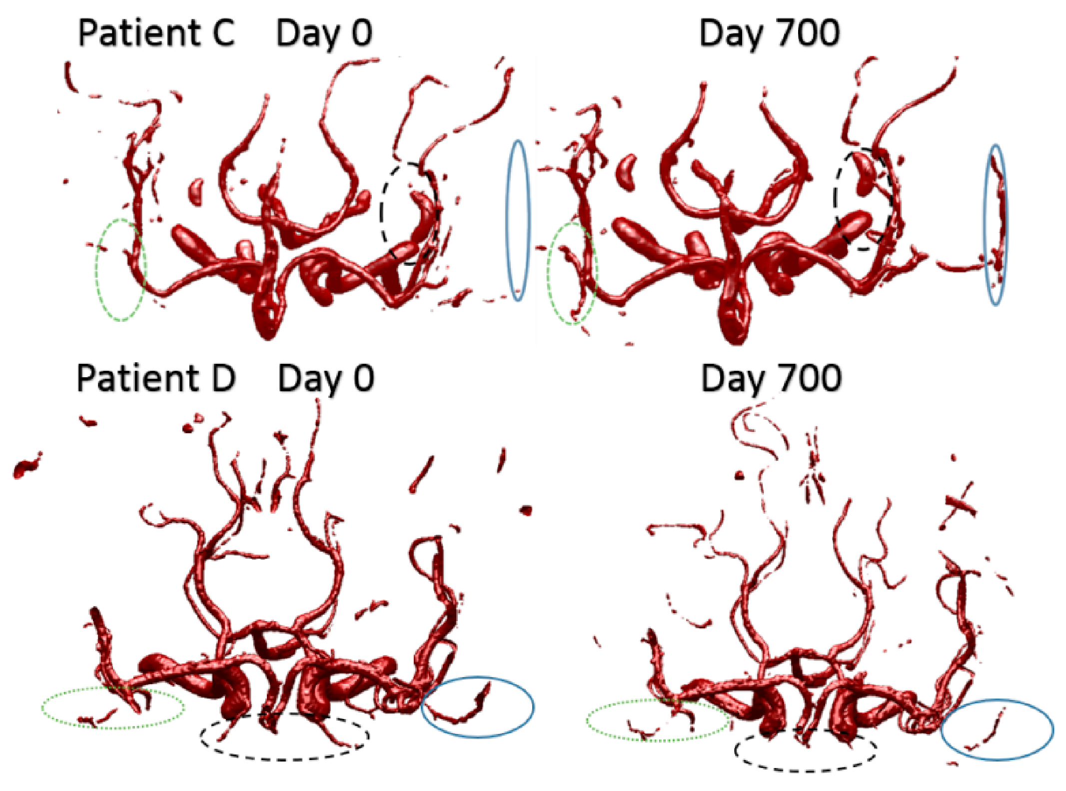
2.4. 3D Reconstruction of the Cerebral Vasculature
3. Results
4. Discussion
5. Limitations
6. Conclusions
Author Contributions
Funding
Institutional Review Board Statement
Informed Consent Statement
Data Availability Statement
Conflicts of Interest
Appendix A
- I.
- Initialization sequentially using EM Algorithm
- II.
- Refining LCDGs using Modified EM Algorithm
References
- CDC. About Underlying Cause of Death, 1999–2015. 2015. Available online: http://wonder.cdc.gov/ucd-icd10.html (accessed on 23 April 2021).
- Mohan, S.; Campbell, N.R. Salt and high blood pressure. Clin. Sci. 2009, 117, 1–11. [Google Scholar] [CrossRef] [PubMed]
- Kulkarni, S.; O’Farrell, I.; Erasi, M.; Kochar, M. Stress and hypertension. WMJ 1998, 97, 34–38. [Google Scholar] [PubMed]
- Sarnak, M.J.; Levey, A.S.; Schoolwerth, A.C.; Coresh, J.; Culleton, B.; Hamm, L.L.; McCullough, P.A.; Kasiske, B.L.; Kelepouris, E.; Klag, M.J.; et al. Kidney disease as a risk factor for development of cardiovascular disease. Circulation 2003, 108, 2154–2169. [Google Scholar] [CrossRef] [PubMed]
- Iadecola, C.; Davisson, R.L. Hypertension and cerebrovascular dysfunction. Cell Metab. 2008, 7, 476–484. [Google Scholar] [CrossRef]
- Van Dijk, E.J.; Breteler, M.M.B.; Schmidt, R.; Berger, K.; Nilsson, L.-G.; Oudkerk, M.; Pajak, A.; Sans, S.; de Ridder, M.; Dufouil, C.; et al. The association between blood pressure, hypertension, and cerebral white matter lesions. Hypertension 2004, 44, 625–630. [Google Scholar] [CrossRef]
- Willmot, M.; Leonardi-Bee, J.; Bath, P.M. High blood pressure in acute stroke and subsequent outcome. Hypertension 2004, 43, 18–24. [Google Scholar] [CrossRef]
- Barnes, J.N.; Harvey, R.E.; Zuk, S.M.; Lundt, E.S.; Lesnick, T.G.; Gunter, J.L.; Senjem, M.L.; Shuster, L.T.; Miller, V.M.; Jack, C.R., Jr.; et al. Aortic hemodynamics and white matter hyperintensities in normotensive postmenopausal women. J. Neurol. 2017, 264, 938–945. [Google Scholar] [CrossRef]
- Jennings, J.R.; Muldoon, M.F.; Ryan, C.; Gach, H.M.; Heim, A.; Sheu, L.K.; Gianaros, P.J. Prehypertensive blood pressures and regional cerebral blood flow independently relate to cognitive performance in midlife. J. Am. Heart Assoc. 2017, 6, e004856. [Google Scholar] [CrossRef]
- Jennings, J.R.; Zanstra, Y. Is the brain the essential in hypertension? Neuroimage 2009, 47, 914–921. [Google Scholar] [CrossRef]
- Launer, L.J.; Lewis, C.E.; Schreiner, P.J.; Sidney, S.; Battapady, H.; Jacobs, D.R.; Lim, K.O.; D’Esposito, M.; Zhang, Q.; Reis, J.; et al. Vascular factors and multiple measures of early brain health: CARDIA brain MRI study. PLoS ONE 2015, 10, e0122138. [Google Scholar] [CrossRef]
- Van der Geest, R.J.; Reiber, J.H. Quantification in cardiac MRI. J. Magn. Reson. Imaging 1999, 10, 602–608. [Google Scholar] [CrossRef]
- Amini, A.A.; Chen, J.; Wang, Y. Imaging and analysis for determination of cardiovascular mechanics. In Proceedings of the 4th IEEE International Symposium on Biomedical Imaging: From Nano to Macro, Arlington, VA, USA, 12–15 April 2007; pp. 692–695. [Google Scholar]
- Van Everdingen, K.; Klijn, C.; Kappelle, L.; Mali, W.; Van der Grond, J. MRA flow quantification in patients with a symptomatic internal carotid artery occlusion. Stroke 1997, 28, 1595–1600. [Google Scholar] [CrossRef]
- Chung, A.C.; Noble, J.A. Statistical 3D vessel segmentation using a Rician distribution. In Proceedings of the International Conference on Medical Image Computing and Computer-Assisted Intervention, Cambridge, UK, 19–22 September 1999; pp. 82–89. [Google Scholar]
- El-Baz, A.; Elnakib, A.; Khalifa, F.; Abou El-Ghar, M.; McClure, P.; Soliman, A.; Gimelrfarb, G. Precise segmentation of 3-D magnetic resonance angiography. IEEE Trans. Biomed. Eng. 2012, 59, 2019–2029. [Google Scholar] [CrossRef]
- Wilson, D.L.; Noble, J.A. An adaptive segmentation algorithm for time-of-flight MRA data. IEEE Trans. Med. Imaging 1999, 18, 938–945. [Google Scholar] [CrossRef]
- Gimel’farb, G.; Farag, A.A.; El-Baz, A. Expectation-Maximization for a linear combination of Gaussians. In Proceedings of the 17th International Conference on Pattern Recognition, Cambridge, UK, 26 August 2004; Volume 3, pp. 422–425. [Google Scholar]
- Forkert, N.D.; Säring, D.; Illies, T.; Fiehler, J.; Ehrhardt, J.; Handels, H.; Schmidt-Richberg, A. Direction-dependent level set segmentation of cerebrovascular structures. In Proceedings of the SPIE Medical Imaging, Orlando, FL, USA, 15 March 2011; p. 79623S. [Google Scholar]
- Holtzman-Gazit, M.; Kimmel, R.; Peled, N.; Goldsher, D. Segmentation of thin structures in volumetric medical images. IEEE Trans. Image Process. 2006, 15, 354–363. [Google Scholar] [CrossRef]
- Xu, C.; Prince, J.L. Snakes, shapes, and gradient vector flow. IEEE Trans. Image Process. 1998, 7, 359–369. [Google Scholar]
- Webb, A.R. Statistical Pattern Recognition; John Wiley amd Sons: Hoboken, NJ, USA, 2003. [Google Scholar]
- Sabry, M.; Sites, C.B.; Farag, A.A.; Hushek, S.; Moriarty, T. A fast automatic method for 3D volume segmentation of the human cerebrovascular. In CARS 2002 Computer Assisted Radiology and Surgery; Springer: Berlin/Heidelberg, Germany, 2002; pp. 382–387. [Google Scholar]
- Suzuki, K. Computerized segmentation of organs by means of geodesic active-contour level-set algorithm. In Multi-Modality State-of-the-Art Medical Image Segmentation and Registration Methodologies; Springer: Berlin/Heidelberg, Germany, 2011; pp. 103–128. [Google Scholar]
- Itai, Y.; Kim, H.; Ishikawa, S.; Katsuragawa, S.; Doi, K. Development of a voxel-matching technique for substantial reduction of subtraction artifacts in temporal subtraction images obtained from thoracic MDCT. J. Digit. Imaging 2010, 23, 31–38. [Google Scholar] [CrossRef][Green Version]
- Jennings, J.R.; Heim, A.F. From brain to behavior: Hypertension’s modulation of cognition and affect. Int. J. Hypertens. 2012, 2012, 701385. [Google Scholar] [CrossRef]
- Gorelick, P.B.; Scuteri, A.; Black, S.E.; Decarli, C.; Greenberg, S.M.; Iadecola, C.; Launer, L.J.; Laurent, S.; Lopez, O.L.; Nyenhuis, D.; et al. Vascular contributions to cognitive impairment and dementia. Stroke 2011, 42, 2672–2713. [Google Scholar] [CrossRef]
- Iadecola, C.; Yaffe, K.; Biller, J.; Bratzke, L.C.; Faraci, F.M.; Gorelick, P.B.; Gulati, M.; Kamel, H.; Knopman, D.S.; Launer, L.J.; et al. Impact of hypertension on cognitive function: A scientific statement from the American Heart Association. Hypertension 2016, 68, e67–e94. [Google Scholar] [CrossRef]
- Whelton, P.K.; Carey, R.M.; Aronow, W.S.; Casey, D.E., Jr.; Collins, K.J.; Himmelfarb, C.D.; DePalma, S.M.; Gidding, S.; Jamerson, K.A.; Jones, D.W.; et al. 2017 ACC/AHA/AAPA/ABC/ACPM/AGS/APhA/ASH/ASPC/NMA/PCNA guideline for the prevention, detection, evaluation, and management of high blood pressure in adults: A report of the American College of Cardiology/American Heart Association Task Force on Clinical Practice Guidelines. J. Am. Coll. Cardiol. 2018, 71, e13–e115. [Google Scholar]
- Warnert, E.A.; Rodrigues, J.C.L.; Burchell, A.E.; Neumann, S.; Ratcliffe, L.E.K.; Manghat, N.E.; Harris, A.D.; Adams, Z.; Nightingale, A.K.; Wise, R.G.; et al. Is high blood pressure self-protection for the brain? Circ. Res. 2016. [Google Scholar] [CrossRef]
- Levy, E.I.; Scarrow, A.M.; Jannetta, P.J. Microvascular decompression in the treatment of hypertension: Review and update. World Neurosurg. 2001, 55, 2–10. [Google Scholar] [CrossRef]
- Friedman, J.; Hastie, T.; Tibshirani, R. The Elements of Statistical Learning; Springer Series in Statistics; Springer: Berlin/Heidelberg, Germany, 2001. [Google Scholar]


| Time | Sensitivity | Specificity |
|---|---|---|
| Day 0 | 0.997 ± 0.006 | 0.9998 ± 0.0001 |
| Day 700 | 0.996 ± 0.008 | 0.9998 ± 0.0001 |
| Cumulative | 0.997 ± 0.008 | 0.9998 ± 0.0001 |
| Mean Vascular Diameter below Circle of Willis | |||
| Effect | χ2 | p-Value | |
| Age | 3.2 μm/y | 0.356 | 0.551 |
| Gender | F > M by 12.8 μm | 0.026 | 0.872 |
| Mean Arterial Pressure | −5.3 μm/mmHg | 11.63 | 0.0007 |
| Mean Vascular Diameter above Circle of Willis | |||
| Effect | χ2 | p-Value | |
| Age | −16.5 μm/y | 12.29 | 0.0005 |
| Gender | F > M by 16.0 μm | 0.199 | 0.655 |
| Mean Arterial Pressure | 1.6 μm/mmHg | 0.402 | 0.525 |
| Patient | Day 0 | Day 700 | ||||
|---|---|---|---|---|---|---|
| Systolic BP | Diastolic BP | MAP | Systolic BP | Diastolic BP | MAP | |
| A | 120 | 80.5 | 93.7 | 103.5 | 66.5 | 78.8 |
| B | 130.5 | 83 | 98.8 | 143.5 | 94 | 110.5 |
| C | 118 | 80.5 | 93 | 105.3 | 69 | 81.1 |
| D | 114 | 84.5 | 94.3 | 120 | 88 | 98.7 |
Publisher’s Note: MDPI stays neutral with regard to jurisdictional claims in published maps and institutional affiliations. |
© 2021 by the authors. Licensee MDPI, Basel, Switzerland. This article is an open access article distributed under the terms and conditions of the Creative Commons Attribution (CC BY) license (https://creativecommons.org/licenses/by/4.0/).
Share and Cite
Taher, F.; Kandil, H.; Gebru, Y.; Mahmoud, A.; Shalaby, A.; El-Mashad, S.; El-Baz, A. A Novel MRA-Based Framework for Segmenting the Cerebrovascular System and Correlating Cerebral Vascular Changes to Mean Arterial Pressure. Appl. Sci. 2021, 11, 4022. https://doi.org/10.3390/app11094022
Taher F, Kandil H, Gebru Y, Mahmoud A, Shalaby A, El-Mashad S, El-Baz A. A Novel MRA-Based Framework for Segmenting the Cerebrovascular System and Correlating Cerebral Vascular Changes to Mean Arterial Pressure. Applied Sciences. 2021; 11(9):4022. https://doi.org/10.3390/app11094022
Chicago/Turabian StyleTaher, Fatma, Heba Kandil, Yitzhak Gebru, Ali Mahmoud, Ahmed Shalaby, Shady El-Mashad, and Ayman El-Baz. 2021. "A Novel MRA-Based Framework for Segmenting the Cerebrovascular System and Correlating Cerebral Vascular Changes to Mean Arterial Pressure" Applied Sciences 11, no. 9: 4022. https://doi.org/10.3390/app11094022
APA StyleTaher, F., Kandil, H., Gebru, Y., Mahmoud, A., Shalaby, A., El-Mashad, S., & El-Baz, A. (2021). A Novel MRA-Based Framework for Segmenting the Cerebrovascular System and Correlating Cerebral Vascular Changes to Mean Arterial Pressure. Applied Sciences, 11(9), 4022. https://doi.org/10.3390/app11094022