Article

Whole Heart Segmentation Using 3D FM-Pre-ResNet Encoder–Decoder Based Architecture with Variational Autoencoder Regularization

Faculty of Electrical Engineering, Computer Science and Information Technology Osijek, 31000 Osijek, Croatia
*
Author to whom correspondence should be addressed.
These authors contributed equally to this work.
Appl. Sci. 2021, 11(9), 3912; https://doi.org/10.3390/app11093912
Submission received: 30 March 2021 / Revised: 20 April 2021 / Accepted: 21 April 2021 / Published: 26 April 2021
(This article belongs to the Special Issue Artificial Intelligence for Medical Image Analysis)

Abstract

:
An accurate whole heart segmentation (WHS) on medical images, including computed tomography (CT) and magnetic resonance (MR) images, plays a crucial role in many clinical applications, such as cardiovascular disease diagnosis, pre-surgical planning, and intraoperative treatment. Manual whole-heart segmentation is a time-consuming process, prone to subjectivity and error. Therefore, there is a need to develop a quick, automatic, and accurate whole heart segmentation systems. Nowadays, convolutional neural networks (CNNs) emerged as a robust approach for medical image segmentation. In this paper, we first introduce a novel connectivity structure of residual unit that we refer to as a feature merge residual unit (FM-Pre-ResNet). The proposed connectivity allows the creation of distinctly deep models without an increase in the number of parameters compared to the pre-activation residual units. Second, we propose a three-dimensional (3D) encoder–decoder based architecture that successfully incorporates FM-Pre-ResNet units and variational autoencoder (VAE). In an encoding stage, FM-Pre-ResNet units are used for learning a low-dimensional representation of the input. After that, the variational autoencoder (VAE) reconstructs the input image from the low-dimensional latent space to provide a strong regularization of all model weights, simultaneously preventing overfitting on the training data. Finally, the decoding stage creates the final whole heart segmentation. We evaluate our method on the 40 test subjects of the MICCAI Multi-Modality Whole Heart Segmentation (MM-WHS) Challenge. The average dice values of whole heart segmentation are 90.39% (CT images) and 89.50% (MRI images), which are both highly comparable to the state-of-the-art.

1. Introduction

Functional irregularities of the heart and blood circulatory system are referred to as cardiovascular diseases (CVDs). CVDs cause significant degeneration of patients’ life quality, while severe cases result in death. Research statistics provided by the World Health Organization show that CVDs account for 17.9 million deaths per year, which makes them the leading cause of death globally [1]. Early diagnosis of CVDs enables timely and appropriate treatment and prevention of patients’ death. The diagnostic process includes obtaining images of unhealthy or weakened heart structures using imaging devices such as echocardiography, computed tomography (CT), or magnetic resonance (MRI). After that, collected images are observed, interpreted, and analyzed by clinical experts using specialized medical software built with advanced image processing methods.
Various clinical applications require insights into different cardiovascular system structures. For example, whole heart segmentation is crucial for pathology localization and hearts’ anatomy and function analysis. The construction of patient-specific three-dimensional (3D) heart models and surgical implants greatly benefits pre-surgical planning for patients with atherosclerosis, congenital heart defects, cardiomyopathy, or even inspecting different heart infections in post-surgical treatment [2]. Whole heart segmentation includes delineation of four heart chambers, the entire blood pool, and the great vessels, which makes manual segmentation by clinical experts time-consuming and prone to observer variability. There is an increasing focus on developing accurate and robust automatic image processing methods. The development of accurate, efficient, and automatic image processing and analysis methods is a complex task, especially in the medical field. The main reason is in high variability in image intensities distribution and dynamic properties of cardiac structures. Nevertheless, the advancements and rapid development in image processing, computer vision, and artificial intelligence fields significantly facilitate this challenging task.
A commonly used approach for medical image segmentation includes encoder–decoder-based architectures such as the U-Net architecture [3]. The U-Net architecture and its’ corresponding three-dimensional counterpart, 3D U-Net [4], consist of contracting and expanding pathways. Throughout the contracting pathway, the network learns low-level features and reduces its numbers using sets of pooling and convolutional layers. In an expanding pathway, the network learns high-level features and recovers the original image resolution using deconvolutional layers. Features from contracting and expanding pathways are concatenated with skip connections to retrieve lost image information that occurs during the down-sampling process. Intuitively, this indicates that the part of the information is lost during the encoding process and can not be recovered when decoding. Variational autoencoders [5] enable regularization during the training to ensure that the latent space, i.e., encoded space, keeps the maximum of information when encoding, which results in the minimum reconstruction error during the decoding. Furthermore, since the number of features in the contracting pathway is significantly lower than the number in the expanding pathway, direct concatenation of these features may not produce the most optimal results. The increment in the number of layers provides larger parameter space enabling learning of more abstract features. Therefore, deeper architectures could provide more abstract learning that results in better performance and higher accuracy in medical segmentation tasks. Common obstacles in training deeper neural network architectures are the appearance of vanishing gradients, accuracy degradations, and extensive parameter growth that lead to computationally expensive models. Recent advancements have shown that convolutional networks can be significantly deeper and still preserve high efficiency and accuracy if they contain shorter and direct connections in between each layer. The introduction of skip connections in ResNets [6] allows for copying of the activations from layer to layer. Since some features are best constructed in shallow networks and others require more depth, skip connections increase the network’s capability, flexibility, and performance.

1.1. Research Contributions

Motivated by previously described advancements, in this paper, we present a novel 3D encoder–decoder based architecture with variational autoencoder regularization. Our intention is to achieve maximum optimality in training performance, efficiency, and final segmentation result accuracy for the whole heart segmentation task. The work contributions can be summarized as:
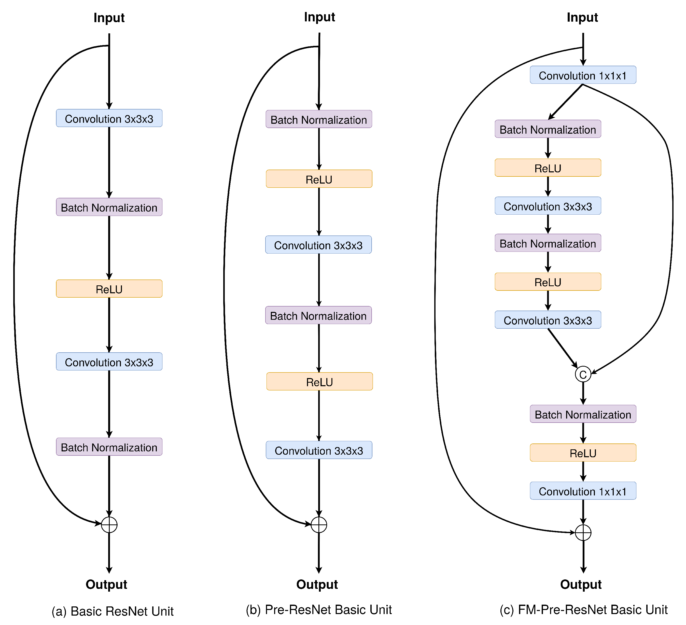
  • We propose a new connectivity structure of residual unit that we refer to as feature merge residual units (FM-Pre-ResNet). The FM-Pre-ResNet unit attaches two convolution layers at the top and at the bottom of the pre-activation residual block. The top layer balances the parameters of the two branches, while the bottom layer reduces the channel dimension. This allows the construction of a deeper model with a similar number of parameters compared to the original pre-activation residual unit.
  • We present a 3D encoder–decoder based architecture that efficiently incorporates FM-Pre-ResNet units and is additionally guided with variational autoencoders (VAE). The architecture includes three stages. First, in an encoding stage, FM-Pre-ResNet units learn a low-dimensional representation of the input. Second, in the VAE stage, an input image is reduced to a low-dimensional latent space and reconstructs itself to provide a strong regularization of all model weights and is only used during the network training. Finally, the decoding stage creates the final whole heart segmentation.
  • The proposed approach obtains highly comparable dice scores to the state-of-the-art for whole heart segmentation tasks on CT images while outperforming the current state-of-the-art on the MRI images.

1.2. Paper Overview

The remainder of the paper is structured as follows. In Section 2, we give an overview of related research. First, we briefly review previous research regarding whole heart segmentation. After that, we provide a background of the most successful ResNet variants and feature reuse mechanisms. Section 3 gives details about our proposed method. First, we introduce an overall architecture design. After that, we present the encoder and decoder stages as well as a theoretical explanation of the new connectivity structure of the residual unit. We introduce the variational autoencoders and their role in the proposed architecture as well. Section 4 provides dataset description, implementation details, and presents conducted experiments and obtained results for the whole heart segmentation. Finally, the concluding remarks are given in Section 5.

2. Related Concepts

In this section, we review some related works. First, we briefly review the prior methods in the whole heart segmentation tasks, focusing on CNN-based approaches. After that, we present significant residual network variants and feature reuse mechanisms relevant to our research.

2.1. Previous Methods for Whole Heart Segmentation

The field of whole heart segmentation is a frequently researched area due to its extremely high importance in clinical practice. Various segmentation algorithms and methods have been proposed over the years. Detail reviews of previously published methodologies can be found in [7,8,9,10]. Prior methods are fundamentally classified into traditional segmentation methods (active contours, deformable models, registration, atlas-based frameworks) and CNN-based segmentation methods. For example, Zhuang et al. [11] propose a new global atlas ranking scheme where both the global and local atlases use the theoretical measures information for computing similarity between the atlases and target image. Galisot et al. [12] propose a method that combines topological graphs and local probabilistic atlases for learning priors. At the same time, the hidden Markov field (MF) integrates the learned information and provides final pixel classification. A significant limitation of registration-based methods is a requirement for high similarity in volume orientation and acquisition protocols between target and atlas images. Recent advancements introduce a simple linear iterative clustering (SLIC) super voxel method for prevention of misregistration by detecting a bounding box region enclosing the heart, after which heart segmentation is performed subsequently [13]. Although registration and atlas-based frameworks usually have high accuracy and precision, algorithms are still not robust enough, which often leads to unsatisfactory results when the data quality is poor.
Recently, CNN-based methods have shown superior performance in the field of medical image segmentation and analysis. For example, Payer et al. [14] use two separate CNNs: first to localize heart and second to segment the fine details of the heart structures within a small region of interest (ROI). The localization network predicts the approximate center of ROI using heatmap regression [15] and the U-Net. Final pixel predictions are acquired using the multi-label segmentation CNN. Wang et al. [16] combine statistical shape priors with CNNs to extract 3D shape knowledge using the shape context method. They detect ROI using a random forest landmark detection, after which they generate a probability map using multi-view slices and three 2D U-Nets. Finally, they apply a hierarchical shape prior algorithm [17] on the probability map to estimate the shape of each heart structure. Sundgaard et al. [18] use 2D CNNs with a multi-planar method to investigate the power of retaining spatial information across slices, as is the case of 3D networks. Mortazi et al. [19] present a multi-planar CNN method using an encoder–decoder architecture. After that, they apply an adaptive fusion [20] to obtain refined segmentation. This method requires less memory in comparison to the 3D counterpart. Liao et al. [21] propose a multi-modality transfer learning method that combines spatial attention mechanism for retaining and removing useful and redundant information, respectively. Furthermore, Dou et al. [22] apply deep supervision during network training to obtain faster convergence and higher distinguishing ability, while Tong et al. [23] combine ROI detection and 3D deeply-supervised U-Net to reduce the computational complexity. Although convolutional neural networks perform well, the limited amount of annotated data requires the development of efficient and more complex, deeper network architectures.

2.2. ResNet Variants and Feature Reuse Networks

Deep convolutional neural networks have shown a significant increase in the accuracy for various segmentation and classification tasks. However, a common obstacle in training deep neural network architectures is the appearance of vanishing or exploding gradients. As the depth of CNN increases, information about the gradient passes through many layers, and it can vanish or accumulate large errors by the time it reaches the end of the network. This problem has been largely addressed using activation functions with a small derivate such as rectified linear unit (ReLU), implementation of gradient clipping, intermediate normalization layers, or careful weight initialization. Nevertheless, with the increasing network depth, accuracy gets saturated and then degrades rapidly. The introduction of skip connections in ResNets [6] allows for copying of the activations from layer to layer, thus preserving information and significantly increasing the performance. Nevertheless, when the depth of the network goes very deep, ResNets become challenging to converge. These difficulties were addressed in Pre-ResNets [24] by introducing forward and backward signals that directly propagate from one block to any other using identity mappings after-addition activation and as the skip-connections. This ultimately constructs a new residual block with the BN-ReLU-Conv order. Zagoruyko [25] introduces level-wise shortcut connections to alleviate the learning capability and significantly boost network performance. Moreover, the deep network initialization problem and incompatibility between ReLU and element-wise summation were addressed in weighted residual networks (WNR) [26]. Although deeper residual networks showed performance improvement, diminishing feature reuse slows down network training. This was addressed by increasing and decreasing the width and depth, respectively, in improved WNRs [27].
Furthermore, another efficient way to alleviate network performance is by reusing features. DenseNet [28] introduces connections between all successive layers in a feed-forward manner where features from each preceding layer are used as inputs to every other layer. This means that each layer is receiving cumulative knowledge from all prior layers, i.e., it reuses features. A variety of compelling benefits are obtained with the introduction of direct connections between layers. First, it allows more depth of the network while simultaneously alleviating the vanishing and exploding gradient problems. Second, the use of features from all layers leads to improvements in the performance. Finally, it efficiently utilizes parameters. This allows for less propensity to overfitting and leads to a reduction of computational costs. CondenseNet [29] combines dense connectivity with a group convolution to further facilitate feature reuse through the network. Here, the group convolutions aim at removing direct connections between layers allowing distinctly smooth feature reuse.

3. Methodology

In this section, we present a theoretical overview of the proposed encoder–decoder based architecture. First, we give an overall architecture design and introduce the main building blocks and their purpose. After that, we give a theoretical background of the main components of our method: feature merge residual units (FM-Pre-ResNet) and variational autoencoder. Finally, we describe the used loss function.

3.1. Architecture Overview

An image segmentation task can be written as mapping:
g ( · ) : I O
where i I denote input images, while o O denote their corresponding segmentations. For an encoder–decoder based architecture, the same mapping function can be written as:
g ( · ) = E Ω ( D Δ ( · ) )
where E Ω , D Δ are an encoder and the decoder networks parametrized by Ω and Δ , respectively. Introduction of shared VAE, expressed with V Λ ( · ) , at the encoders’ endpoint allows mapping of input images to a lower-dimensional latent, i.e., encoded, space. The output of an encoder E Ω contains the samples from the latent space, which we in detail discuss in Section 3.3.
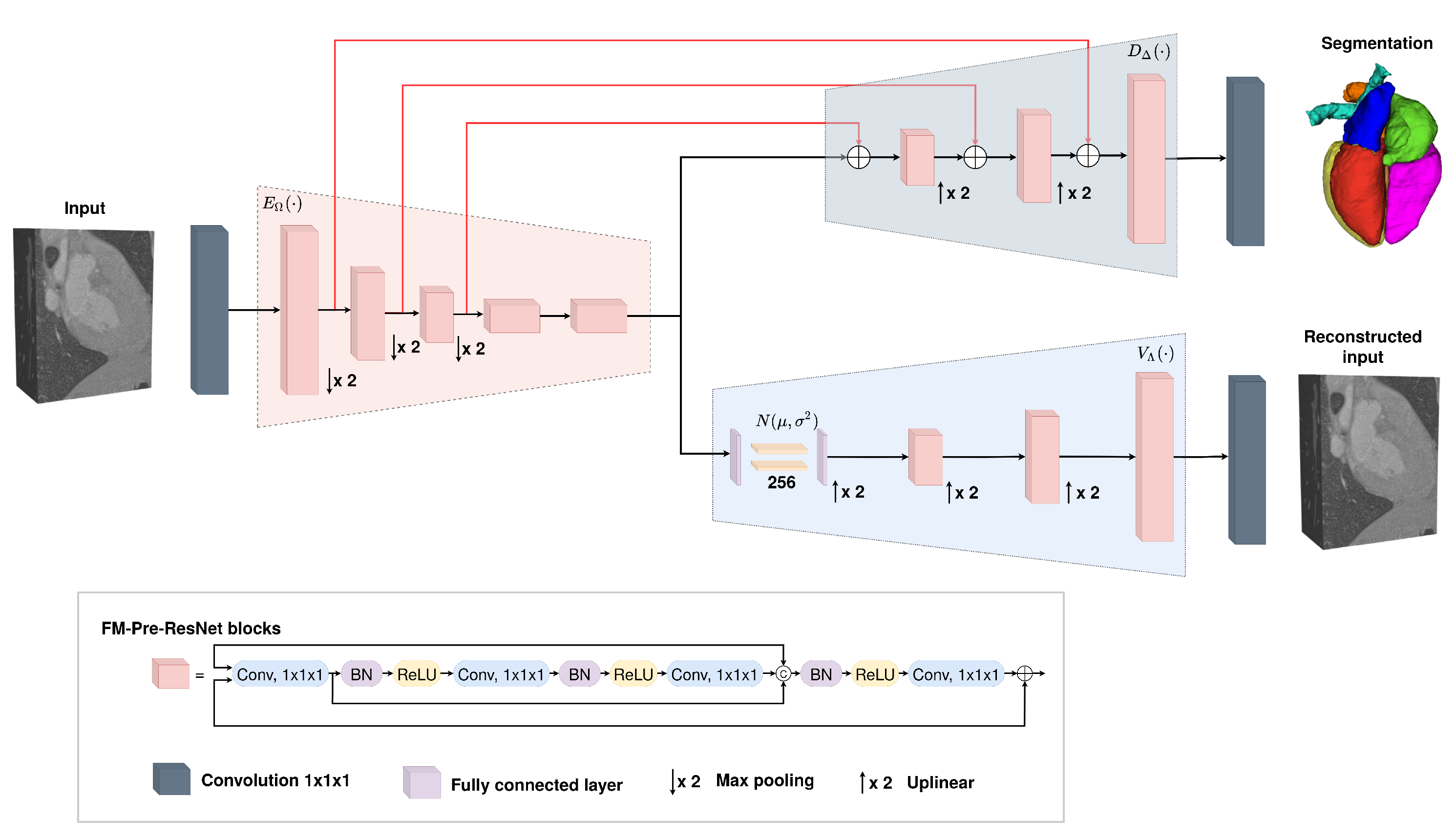
Therefore, our proposed architecture consists of three main stages: (1) encoding stage, (2) reconstruction of the input with variational autoencoder, and (3) decoding stage. An encoding stage incorporates feature merge residual units by which the network learns a low-dimensional representation of the input. The variational autoencoder reconstructs the input image from low-dimensional latent space to regularize all model weights and adds additional guidance to the encoding stage. Finally, in the decoding stage, the network learns high-level features and creates the final segmentations. An illustration of the proposed architecture is shown in Figure 1.

3.2. Encoding Stage

The ResNets contains multiple stacked residual units. Generally, each residual unit can be expressed with the following two formulations:
y l = H ( x l ) + F ( x l , W l ) ,
and
x l + 1 = f ( y l ) ,
where F is residual function, x l and x l + 1 denote the input and output of the l t h residual unit in the network, while the output of the l t h residual unit is denoted with y l . The parameters of the l t h residual unit are denoted as W l , while the function f refers to the rectified linear unit (ReLU).
The identity mapping, by which ResNets learn residual function F in regard to H ( x l ) , can be written as:
H ( x l ) = x l
Therefore, the identity mapping of original residual block attaches an identity skip connection allowing information flow within a residual unit as shown in Figure 2a. As introduced in Pre-ResNets (Figure 2b), if H ( x l ) and f are both an identity mapping, the direct propagation of information through the entire network in forward and backward fashion can be written as:
x l + 1 = H ( x l + F ( x l , W l ) )
Following the concept described in Equation (6), we propose a novel feature merge residual unit that can be written as follows:
Z ( x l ) = F ( z ( x l ) , W l ) z ( x l ) )
and
x l + 1 = H ( x l + g ( Z ( x l ) , W l )
where ∘ presents the concatenation operation, Z ( x l ) denotes the concatenated result, while the functions z and g denote the convolution layers, added at the top and at the bottom of the residual unit, respectively. In this manner, the top convolution layers’ output is concatenated with the residual signals’ output, which allows the merge of features from preceding layers. After that, the concatenated result is passed through a bottom convolution layer to reduce channel dimension, as shown in Figure 2c.

3.3. Variational Autoencoder Stage

Variational autoencoders are able to capture latent representations, which makes them ideal for use in generative settings [5,30]. The evidence lower bound (ELBO), which is VAEs optimization objective, can be written as:
L V A E ( i , i ^ ) = L R E C ( i , i ^ ) + K , L [ q Λ ( r | i ) | | p ( r ) ]
where the term L R E C ( i , i ^ ) denotes reconstruction loss, and can be further written as:
L R E C ( i , i ^ ) = E q r | i [ l o g ( p Δ ( i | r ) ) ]
where i ^ denotes the reconstructed input.
The term K , L [ q Λ ( r | i ) | | p ( r ) ] from Equation (9) defines the K L divergence of the approximating variational density, which can be expressed as:
q Λ ( r | i ) = N ( r ; μ Λ , σ Λ 2 )
The standard prior on the latent variable can be written as:
p ( r ) = N ( r ; 0.1 )
where the aligned Gaussian ( μ Λ , σ Λ 2 ) is expressed by the encoder network V Λ ( · ) .
Following this, the low dimensional representations of the input data i can be obtained by introducing the latent random variable r . The input images are mapped to a low dimensional space using VAE encoder V Λ ( · ) . After that, the output of the encoder of the segmentation network, E Ω ( · ) , takes samples from the latent space as shown in Figure 1. In this manner, segmentation encoder and VAE jointly share the decoder D Δ ( · ) , which can be also written as:
L ( o , o ^ ) = L R E C ( o , s ^ ) + KL [ q Λ ( r | i ) | | p ( r ) ]
The final segmentation, o ^ , is obtained from the decoder using following expression:
o ^ = D Δ [ E Ω ( i ) V Λ ( i ) ]
which can be written as:
o ^ = D Δ [ h r ]
where ∘ denotes concatenation, H = E Ω ( i ) is the output of the segmentation encoder and r q Λ ( r | i ) is a sample from the latent space that is learnt by VAE.

Loss Function

The loss function plays an important role in improving the models’ performance. In this work, we employ total loss function that is the addition of soft dice loss, L 2 loss and standard VAE penalty term, and can be written as:
L = L d i c e + 0.1 · L L 2 + 0.1 · L K L
The term that represents the soft dice loss, L d i c e [31], can be written as:
L d i c e = 2 · P g t · P p r e d p g t 2 + p p r e d 2 + ϵ
where ϵ denotes a small constant used for computational stability, i.e., to avoid zero division.
The loss L 2 represents loss on the VAE encoder output and can be written as:
L L 2 = | | I i n p u t I p r e d | | 2 2
The standard VAE penalty term, L K L , represents K L divergence between a prior distribution N ( 0 , 1 ) and the estimated normal distribution N ( μ , σ 2 ) , which can be written as:
L K L = 1 N μ 2 + σ 2 l o g σ 2 1
where N represents the entire set of image voxels. Finally, the hyperparameter weight of 0.1 is empirically found to provide a good balance between VAE loss term and soft dice loss in Equation (16).

3.4. Decoding Stage

The decoder building blocks highly follows concepts described in Section 3.2, i.e., it consists of FM-Pre-ResNet units. Every FM-Pre-ResNet unit in decoder doubles the spatial dimension while reduces the feature numbers by a factor of 2. Each decoder level is concatenated with the corresponding encoder output. The final layer of the decoder provides whole heart segmentation and has the same number of features and spatial size as the original input image.

4. Implementation Details

In this section, we give a dataset description on which we conducted our experiments. After that, we give details about network training and implementation. Finally, we evaluate the proposed method using Multi-Modality Whole Heart Segmentation Challenge (MM-WHS) dataset and present conducted experiments and results. We investigate and compare our results to the state-of-the-art research.

4.1. Dataset Description

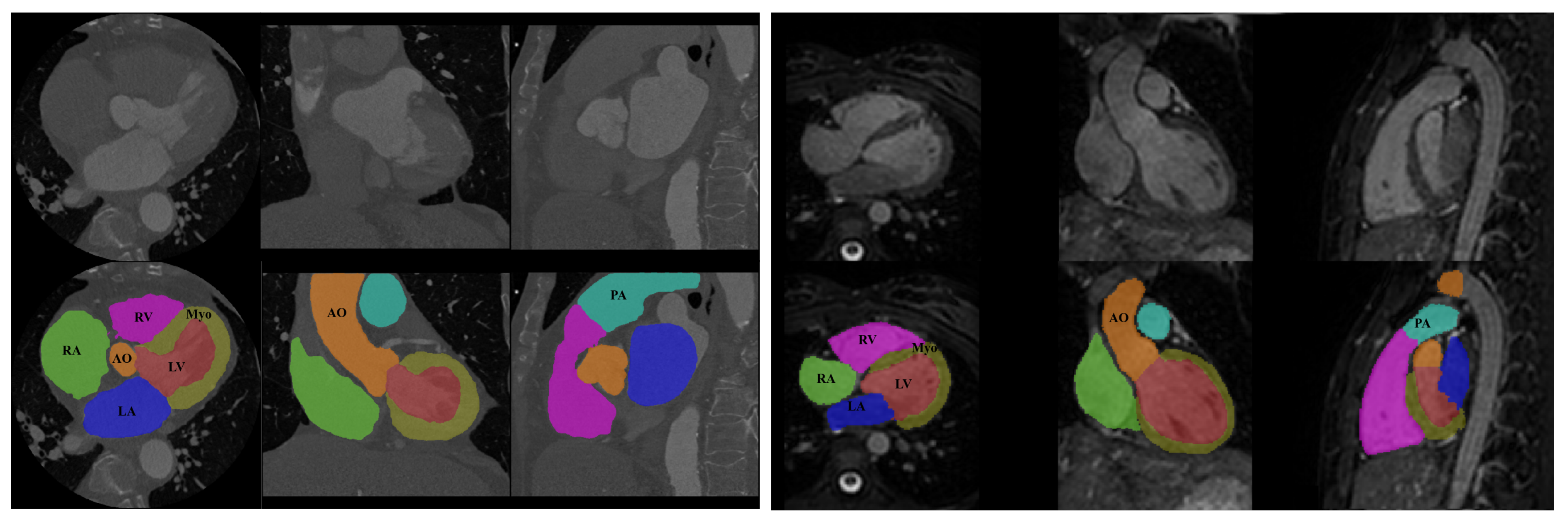
The network presented in the previous section was applied to the whole heart segmentation task and is evaluated on a dataset provided by Multi-Modality Whole Heart Segmentation Challenge (MM-WHS) organized by MICCAI [32]. The MM-WHS dataset consists of 60 cardiac CT/CTA and 60 cardiac MRI volumes, whereas 20 volumetric images include corresponding ground truths, manually labeled by two clinical experts. In contrast, the remaining 40 volumetric images are used for testing purposes. Ground truths of the testing dataset are provided in encrypted form and can be decoded to evaluate algorithms using the procedure described in [32]. The data were collected on patients from the everyday clinical environment, and it has a various quality to preserve the robustness of the developed algorithms when it comes to real clinical usage. The cardiac CT/CTA data are obtained using 64 slice CT scanners using a standard coronary CT angiography protocol, and cardiac MRI data were acquired using a navigator-gated 3D balanced steady-state free precession (b-SSFP) sequence for free-breathing whole heart imaging. The axial slices’ in-plane resolution is 0.78 × 0.78 mm, and the average slice thickness is 1.60 mm. The data include the following seven structures of the heart: (1) the left ventricle blood cavity (LV), (2) the right ventricle blood cavity (RV), (3) the left atrium blood cavity (LA), (4) the right atrium blood cavity (RA), (5) the myocardium of the left ventricle (Myo), (6) the ascending aorta (Ao), which is defined as the aortic trunk from the aortic valve to the superior level of the atria, and (7) the pulmonary artery (PA). An example of one slice from the used dataset is shown in Figure 3.

4.2. Training and Implementation Details

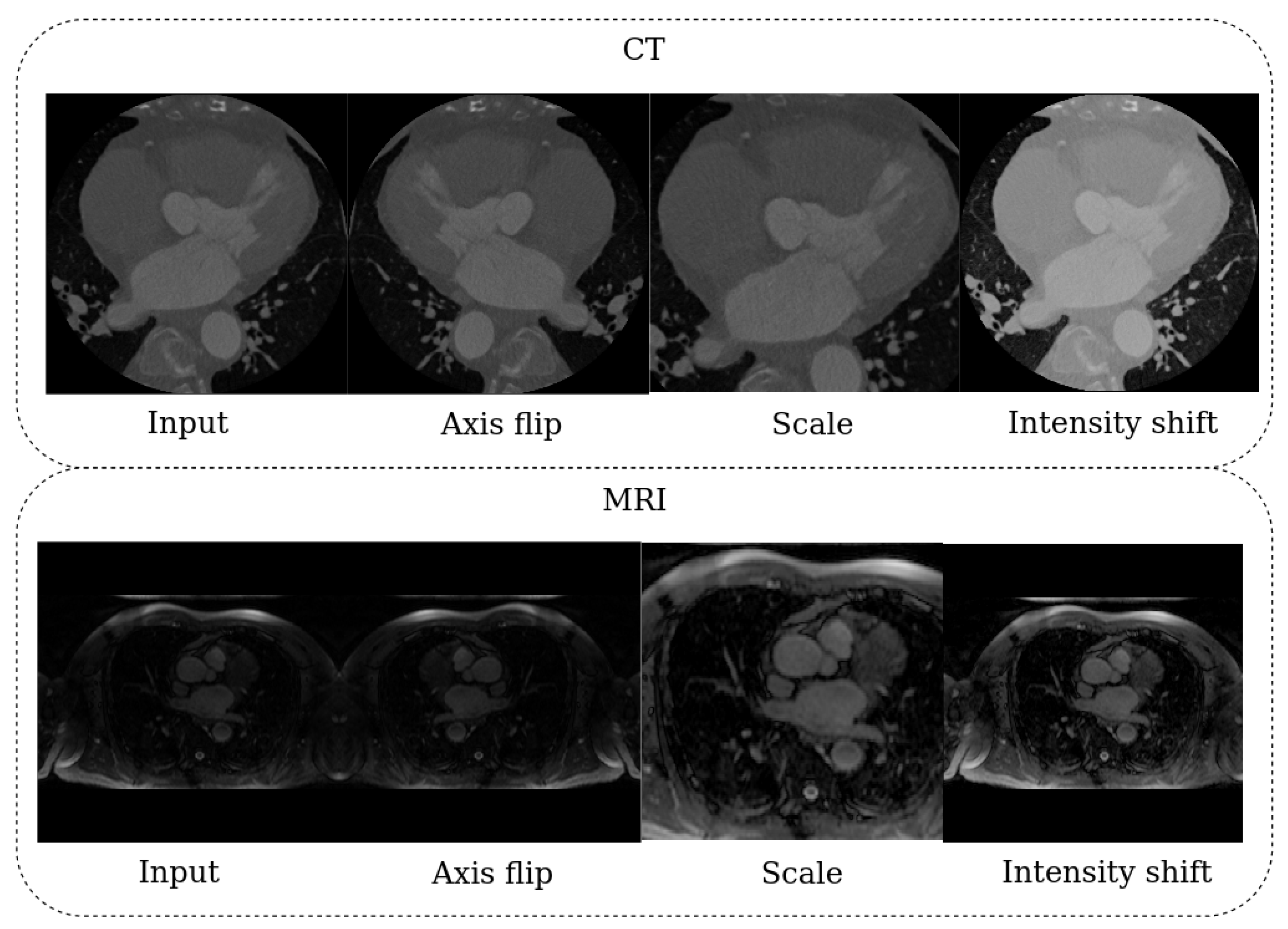
To alleviate the irregularities of variable contrast in some MRI images, we normalize all input images (both CT and MRI) to have zero mean and unit std. The volumes were cropped and zero-padded to a fixed size of 176 × 224 × 144 to provide a fine ROI for the network input while making sure all heart structures are inside the selected ROI. We apply three different data augmentation methods on input image channels to increase the sample size of training data and enhance the robustness and generalization ability, namely random axis mirror flip, random scaling, and intensity shift. Random axis mirror flip creates a mirror reflection of an original image along one (or more) selected axis and is commonly flipped at a rate of 50%. Random scaling operation S scales input image and performs independently in different directions. Intensity shift performs an element-wise addition of a scalar to the image and affects the brightness of the original image. Details about parameters of used data augmentation methods are presented in Table 1 while examples of input images after applying different data augmentation methods are shown in Figure 4. Moreover, we empirically found that advanced augmentation techniques, such as random histogram matching, or random image filtering, do not show any additional improvements to the final segmentation result.
While optimization methods such as stochastic gradient descent (SGD) or gradient descent with momentum provide a powerful optimization for training CNNs, choosing the most optimal learning rate α is not a trivial task. If α is chosen to be too large, the training may not converge, might oscillate, or skip over relevant local minima. On the other hand, if it is chosen to be too small, it significantly delays the convergence process. Therefore, in this work, we use adaptive learning rate optimizer Adam with initial learning rate of α 0 = 10 4 and gradually decrease it according to the following expression:
α = α 0 * 1 c T c 0.9
where T c is a total number of epochs (200 in our case) and c is an epoch counter. Furthermore, to ensure our models generalizes well on unseen data, i.e., to reduce the effect of overfitting or underfitting, we employ L 2 norm regularization with a weight of 10 5 and the spatial dropout with a rate of 0.2 after the initial encoder convolution. Since early stoping aims to regularize the finding the network parameters at the point of the lowest validation loss, we implement early stopping with patience set to 50.
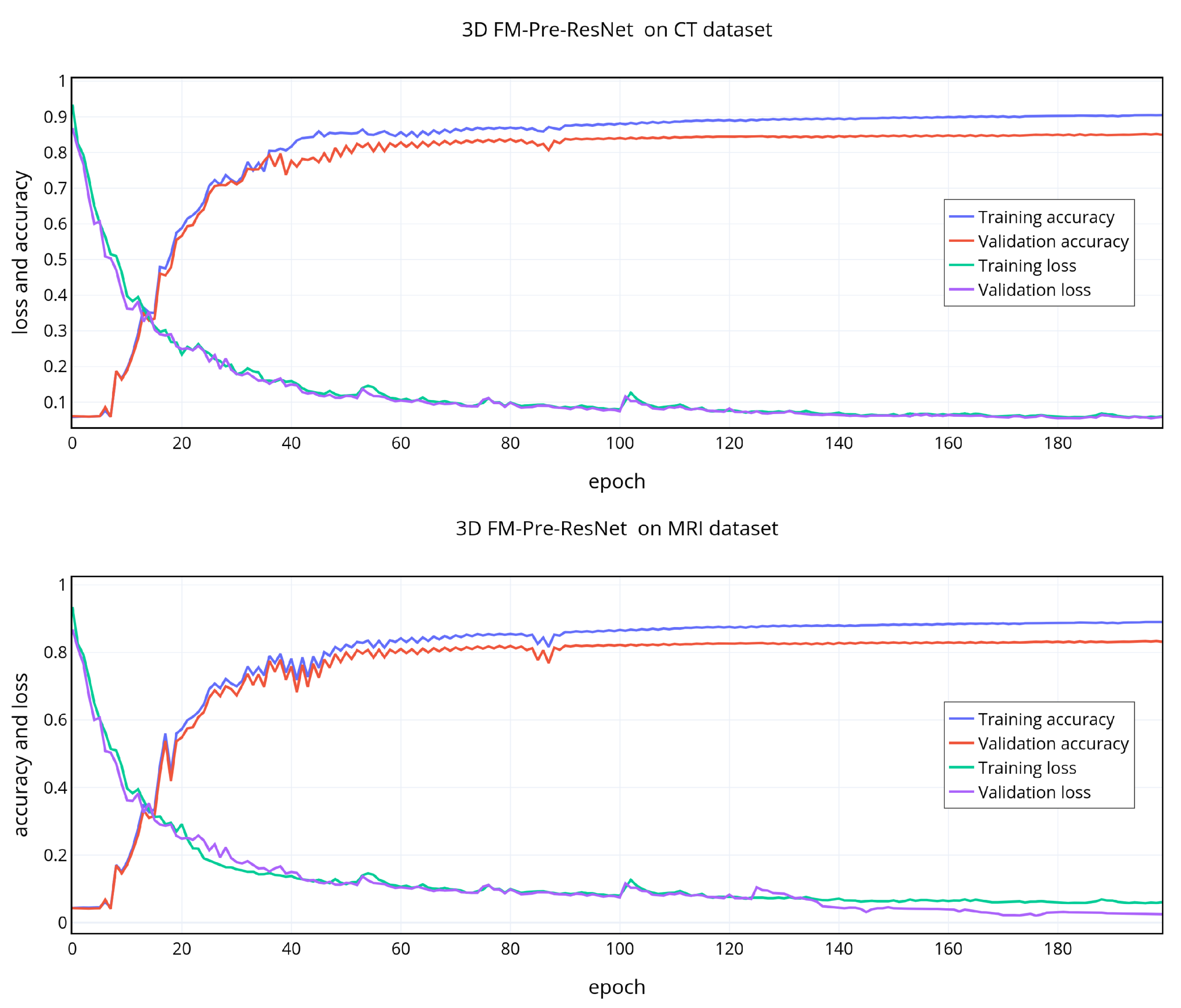
In our experiments, we train four encoder–decoder based architectures: (1) 3D Pre-ResNet without VAE regularization, (2) 3D Pre-ResNet with VAE regularization, (3) FM-Pre-ResNet without VAE regularization, and (4) FM-Pre-ResNet with VAE regularization. All four networks are trained from scratch and separately for CT and MRI images. The whole experimental procedure is implemented in Pytorch and trained on two NVIDIA Titan V GPU simultaneously. The source code of our method is available at [33]. Our training and validation dataset consists of 20 CT volumes and 20 MRI volumes, with 80 20 % training and validation split, respectively. The trained networks are evaluated using a testing dataset that includes 40 subjects for both CT and MRI images. The proposed 3D FM-PreResNet + VAE architecture produced the highest validation accuracy of 94.40% at the end of the 200th epoch. The network is trained for 200 epochs since further training appears not to decrease validation loss as shown in Figure 5. Moreover, Figure 5 shows that, with an increase in epochs, the loss value decreases, and the accuracy increases. This is a clear indication that the network is successfully learning from the input data.

4.3. Evaluation Metrics

To evaluate the proposed methodologys’ performance, we compare ground truth masks with obtained segmentations for each CT and MRI volume. We used four different metrics to evaluate segmentation accuracy, namely, the Dice similarity coefficient (DSC), Jaccard Index (JI), surface distance (SD), and Hausdorff distance (HD). DSC and JI measure the level of overlap between the ground truth and predicted segmentations, while SD and HD examine boundary distances. The DSC metric measures the degree of overlap between the ground truth and predicted segmentation. It is a commonly used metric for evaluating segmentation quality and can be written as:
D S C ( G , P ) = 2 | G P | | G | + | P |
where G is the ground truth, and P is the predicted mask.
Similarly, the Jaccard Index (JI) emphasizes the size of the intersection divided by the size of the union of the sample sets. The mathematical representation of the JI can be written as:
J I ( G , P ) = | G P | | G P |
where G is the ground truth, and P is the predicted mask.
SD measures an average of the minimum voxel-wise distance between the ground truth and predicted object boundaries and can be written as:
S D ( G , P ) = 1 n G + n P x P P d ¯ ( x P , G ) + d ¯ ( x G , P )
where n G and n P denote the number of voxels on the object boundaries in the ground truth and predicted segmentations, respectively.
Furthermore, HD represents the maximum of the minimum voxel-wise distances between the ground truth and predicted object boundaries and can be written as:
H D ( G , P ) = max g G min p P g 2 p 2
where g is the ground truth, and p is the predicted mask.

5. Experiments and Results

To demonstrate the effectiveness of the proposed approach and our design choice for the new FM-ResNet unit, we train encoder–decoder based architecture using 3D Pre-ResNet without and with VAE regularization as well as the proposed FM-Pre-ResNet without and with VAE regularization.
Table 2 summarizes an average whole heart segmentation results on CT and MRI images. On CT images, the 3D Pre-ResNet network achieves average WHS segmentation results for DSC, JI, SD, and HD of 87.11 % , 80.16 % , 1.71 mm, and 24.44 mm, respectively. The addition of VAE at Pre-ResNet segmentation encoders’ endpoint improve DSC, JI, SD and HD values for 2.12 % , 1.0 % , 0.2039 mm, and 2.704 mm, respectively.
The 3D FM-Pre-ResNet network achieves DSC, JI, SD, and HD values of 90.03 % , 82.14 % , 1.43 mm, and 18.82 mm, respectively. Compared to the 3D Pre-ResNet, it achieves improvement in DSC, JI, SD, and HD values of 2.92 % , 1.98 % , 0.2789 mm, and 56,307 mm, which means that the proposed FM-PreResNet unit significantly improves segmentation accuracy. Moreover, the highest DSC, JI, SD, and HD are achieved using 3D FM-Pre-ResNet + VAE network and report values of 90.39 % , 82.24 % , 1.1093 mm, and 15.3621 mm, respectively.
Similarly, on MRI images, the 3D Pre-ResNet network achieves average WHS segmentation results for DSC, JI, SD, and HD of 83.06 % , 75.54 % , 5.9201 mm, and 42.5578 mm, respectively. The addition of VAE at Pre-ResNet segmentation encoders’ endpoint improve DSC, JI, SD, and HD values for 2.28 % , 0.09 % , 2.15 mm 3.6766 mm.
The 3D FM-Pre-ResNet network achieves average DSC, JI, SD, and HD values of 88.40 % , 78.55 % , 2.4558 mm, and 32.0451 mm, respectively. Compared to 3D Pre-ResNet, it achieves improvement in DSC, JI, SD, and HD values of 5.34 % , 3.01 % , 3.4643 mm, and 10.5127 mm, which means that the proposed FM-PreResNet unit significantly improves segmentation accuracy. Moreover, the highest DSC, JI, SD, and HD are achieved using 3D FM-Pre-ResNet + VAE network and report values of 89.50 % , 80.44 % , 1.8599 mm and 25.6558 mm, respectively. These results highlight the improvement in segmentation accuracy afforded by the introduction of FM-Pre-ResNet units and VAE.
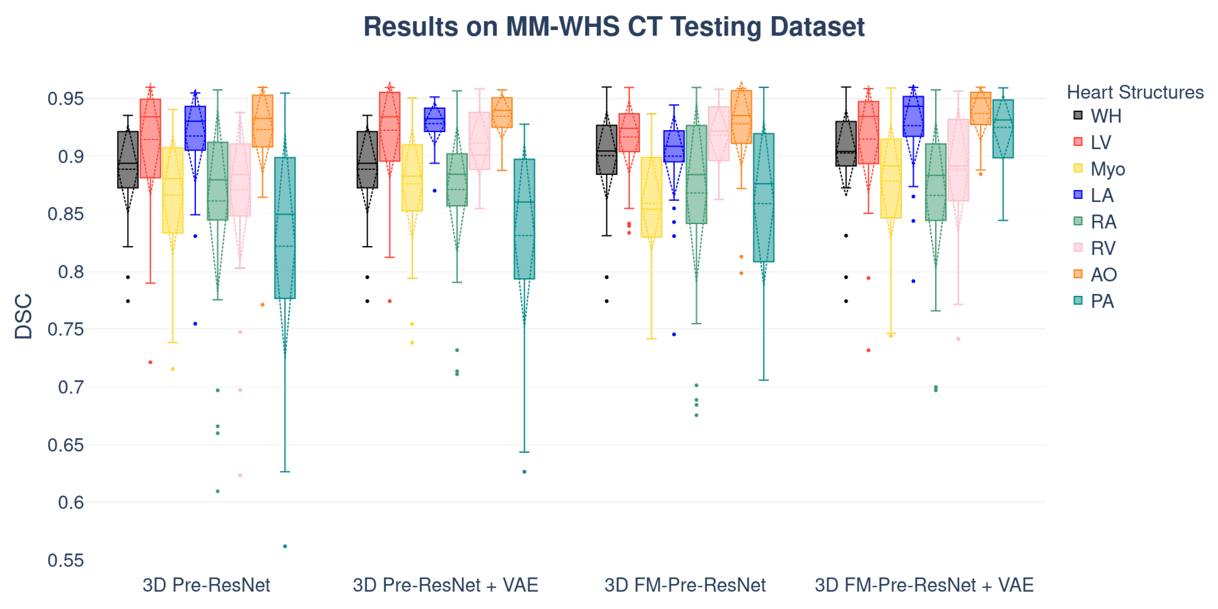
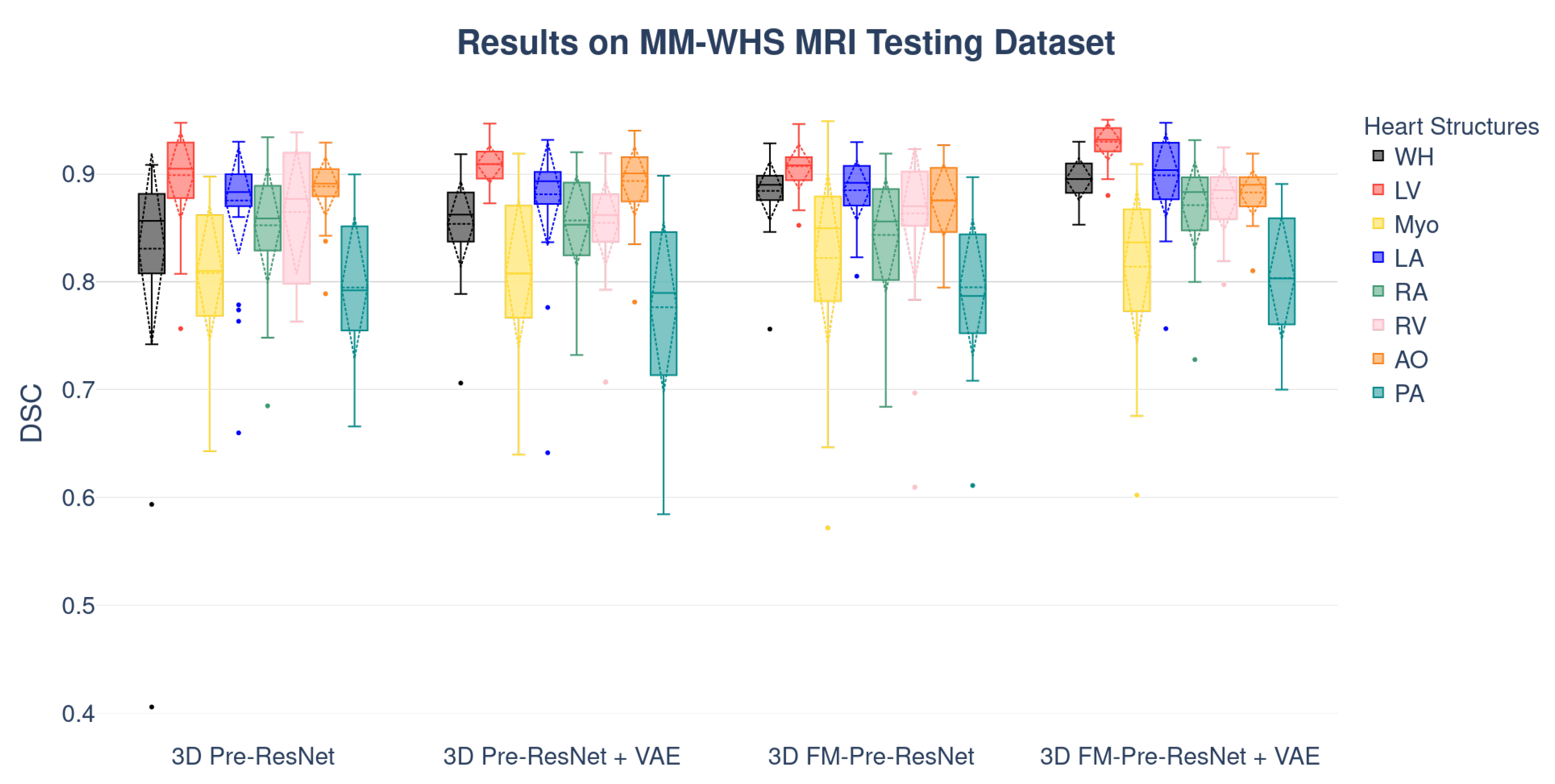
Boxplots showing the distribution of the DSC for WH, LV, Myo, LA, RA, RV, AO, and PA using different segmentation networks on MMWHS CT and MRI testing datasets are presented in Figure 6 and Figure 7, respectively. Additional, structure-wise segmentation accuracies for the LV, RV, LA, RA, Myo, Ao, and PA, for both CT and MRI images, are summarized in Table 3 and Table 4.
The p-values have been calculated using a Wilcoxon rank-sum test to show the significant difference of used architectures. Bonferroni correction was used for controlling the family-wise error rate. Figure 8 and Figure 9 show the comparisons and p-values for CT and MRI testing datasets, respectively.
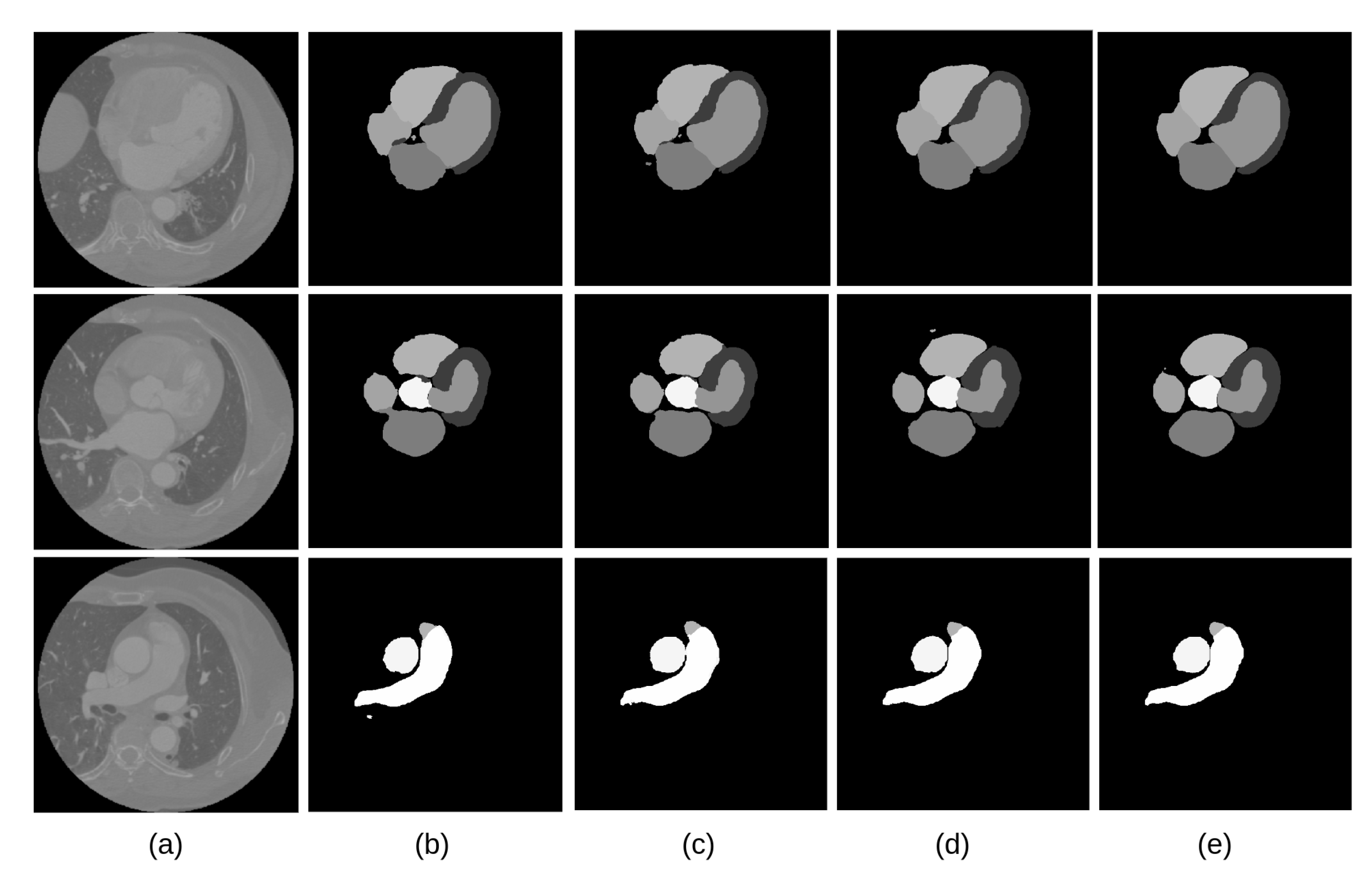
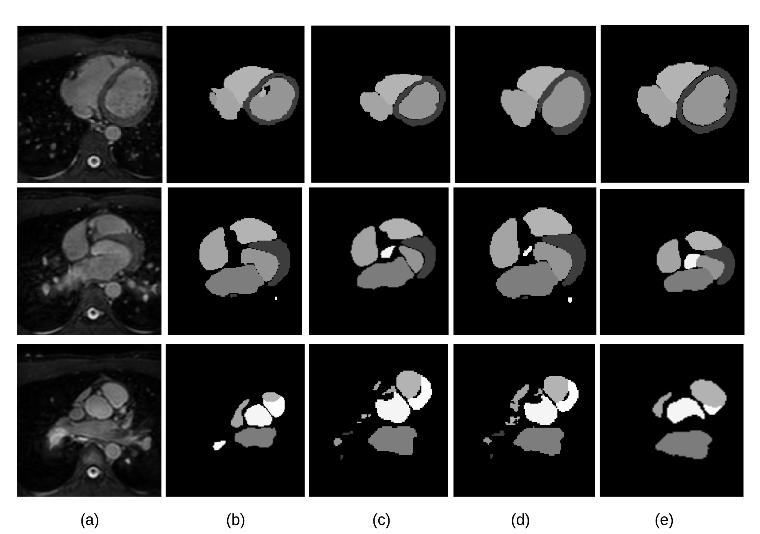
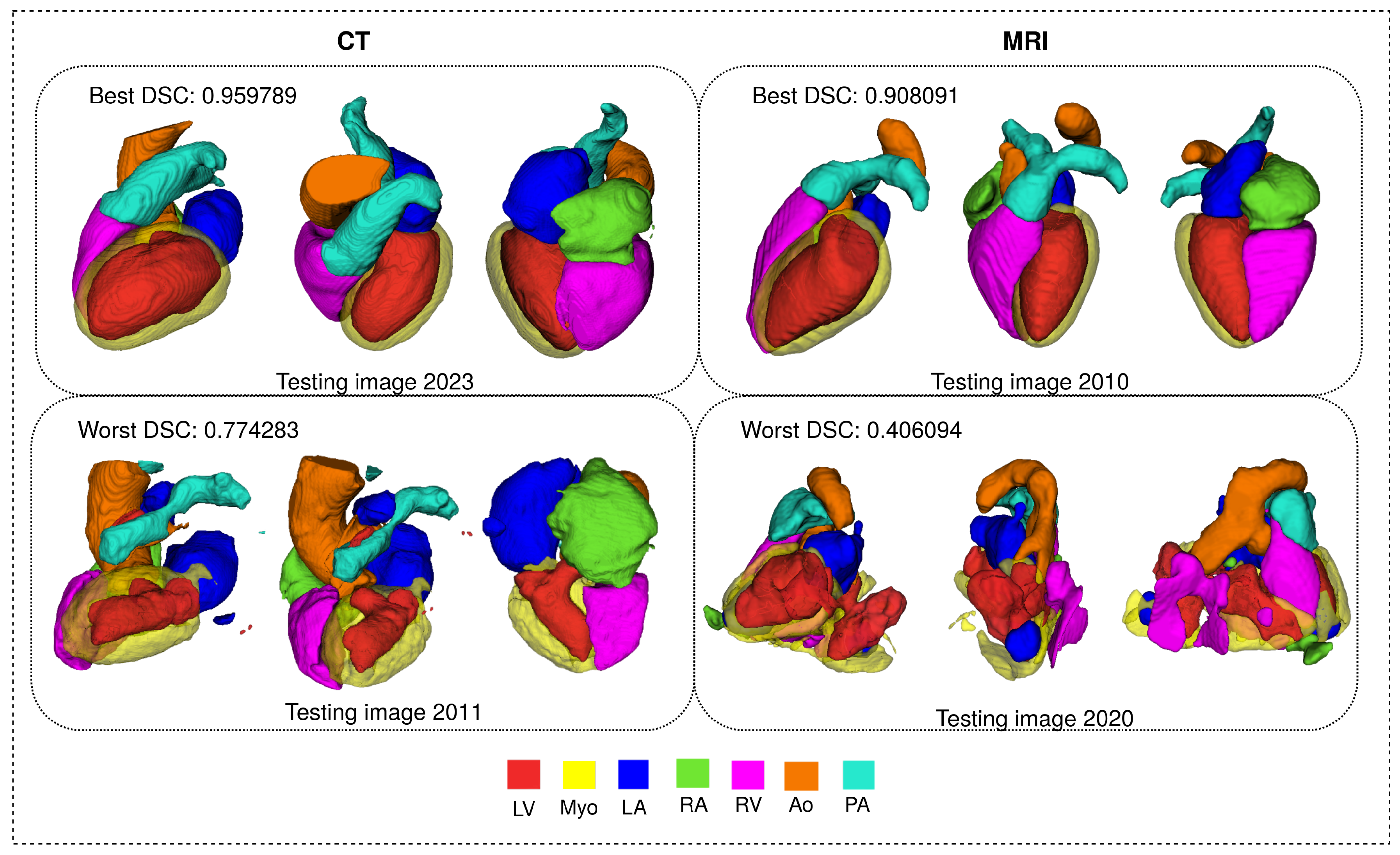
The visual inspection of the obtained segmentations using each network investigated in this work is presented in Figure 10 for the CT dataset, and Figure 11 for the MRI dataset. For example, Figure 11d shows clear improvements regarding LV segmentation that is obtained using FM-Pre-ResNet compared to missed segmentation of LV parts while using Pre-ResNet without a proposed feature merge residual unit as shown in Figure 11b. Moreover, Figure 11e shows a significant reduction in segmentation error compared to all other presented networks. This further highlights the benefits of the proposed FM-Pre-ResNet + VAE approach. Nonetheless, in both modalities, PA and Myo’s segmentation results are significantly lower than other substructures due to high shape variations and heterogeneous intensity of blood fluctuations. Figure 12 shows 3D visualization of the best and the worse segmentation cases on the CT and MRI test dataset obtained using the proposed FM-Pre-ResNet +VAE approach.
Furthermore, Pre-ResNet has demonstrated that increasing the depth of the network improves model performance significantly. The addition of two convolutional layers at the top and bottom of the pre-activation residual block introduced in our FM-Pre-ResNet unit allows for the feature fusion block to reach the same depth with fewer parameters which benefits model performance. Therefore, the proposed type of connectivity of the FM-Pre-ResNet unit in terms of depth and number of parameters regarding Pre-ResNet implies no increase in the number of parameters compared to the Pre-ResNet. Time-wise, each training epoch (200 cases) and prediction times on two GPU-s (NVIDIA Titan V) are significantly reduced with architectures with VAE. This shows the computational efficiency of our choice for VAE introduction. Comparison of depth, number of parameters, training times per epoch, and prediction time of one volume for different architectures is shown in Table 5.

Comparison with State-of-the-Art Methods

The proposed approach was compared with other similar deep learning approaches in terms of image segmentation accuracy as shown in Table 6 and Table 7. An approach that combines atlas registration with CNNs’ [12] provides an incremental segmentation that allows user interaction, which can be beneficial in a clinical setting. Nevertheless, the challenges of accurate atlas registration resulted in low accuracy on MRI images. The deep supervision mechanism [23] and use of transfer learning [21] result in an increase of trainable parameters and overall network complexity. In contrast, we aim to introduce a light-weight network that results in a significantly deep network without increasing the parameter number. Moreover, the authors in [21] report an average WHS DSC of 0.914 ± 0.075 on CT images and 0.890 ± 0.054 on MRI images using a hold-out set of 10% of training data and evaluate their method with 10-fold cross-validation. Our results report 0.9039 ± 0.0517 on CT images and 0.8950 ± 0.0215 on MRI images and are evaluated on all unseen 40 subjects, which shows that the VAE stage’s introduction significantly helps in overcoming overfitting problems. Therefore, these results highlight the advantages of our proposed method.

6. Conclusions

This paper introduced an efficient encoder–decoder-based architecture for whole heart segmentation on CT and MRI images. Accurate heart and its substructures segmentation enable faster visualization of target structures and data navigation, which benefits clinical practice by reducing diagnosis and prognosis times. Our proposed method introduces a novel connectivity structure of residual unit that we refer to as feature merge residual unit (FM-Pre-ResNet). The proposed connectivity allows the creation of distinctly deep models without an increase in the number of parameters compared to the Pre-ResNet units. Furthermore, we construct an encoder–decoder-based architecture that incorporates the VAE encoder at the segmentation encoder output to have a regularizing effect on the encoder layers. The segmentation encoder learns a low-dimensional representation of the input, after which VAE reduces the input to a low-dimensional space of 256 (128 to represent std, and 128 to represent mean). A sample is then drawn from the Gaussian distribution with the given std and mean and reconstructed into the input image dimensions following the same architecture as the decoder but without inter-level skip connections. Therefore, VAE acts as a regulator of model weights, adds additional guidance, and exploits the encoder endpoint features. In the end, the segmentation decoder learns high-level features and creates the final segmentations. We evaluate the proposed approach on MMWHS CT and MRI testing datasets and obtain average WHS DSC, JI, SD, and HD values of 90.39 % , 82.24 % , 1.1093 , 15.3621 for CT images, and 89.50 % , 80.44 % , 1.8599 , 25.6558 for MRI images, respectively. Results for both datasets are highly comparable to the state-of-the-art.
Author Contributions

M.H.: Conceptualization, methodology, development, writing—original draft, editing; I.G.: Conceptualization, methodology, development, writing original draft, supervision; H.L.: Editing, validation, visualization; K.R.: Editing, validation, visualization. All authors have read and agreed to the published version of the manuscript.

Funding

This research received no external funding.

Data Availability Statement

Source code of our work is available at https://github.com/mhabijan/whs_segmentation (accessed on 17 April 2021).

Acknowledgments

This work has been supported in part by the Croatian Science Foundation under the project UIP-2017-05-4968.

Conflicts of Interest

The authors declare no conflict of interest.

References

  1. World Health Organization. Cardiovascular Diseases Statistics. 2017. Available online: https://www.who.int/cardiovascular_diseases/about_cvd/en/ (accessed on 19 January 2021).
  2. Hibino, N. Three Dimensional Printing: Applications in Surgery for Congenital Heart Disease. World J. Pediatr. Congenit. Heart Surg. 2016, 7, 351–352. [Google Scholar] [CrossRef] [PubMed]
  3. Ronneberger, O.; Fischer, P.; Brox, T. U-Net: Convolutional Networks for Biomedical Image Segmentation. In Medical Image Computing and Computer-Assisted Intervention—MICCAI 2015; Navab, N., Hornegger, J., Wells, W.M., Frangi, A.F., Eds.; Springer International Publishing: Cham, Switzerland, 2015; pp. 234–241. [Google Scholar] [CrossRef] [Green Version]
  4. Çiçek, Ö.; Abdulkadir, A.; Lienkamp, S.S.; Brox, T.; Ronneberger, O. 3D U-Net: Learning Dense Volumetric Segmentation from Sparse Annotation. arXiv 2016, arXiv:1606.06650. [Google Scholar]
  5. Kingma, D.P.; Welling, M. Auto-Encoding Variational Bayes. arXiv 2014, arXiv:1312.6114. [Google Scholar]
  6. He, K.; Zhang, X.; Ren, S.; Sun, J. Deep Residual Learning for Image Recognition. In Proceedings of the 2016 IEEE Conference on Computer Vision and Pattern Recognition (CVPR), Las Vegas, NV, USA, 26 June–1 July 2016; pp. 770–778. [Google Scholar]
  7. Zhuang, X.; Shen, J. Challenges and Methodologies of Fully Automatic Whole Heart Segmentation: A Review. J. Healthc. Eng. 2013, 4, 371–407. [Google Scholar] [CrossRef] [PubMed] [Green Version]
  8. Evaluation of Algorithms for Multi Modality Whole Heart Segmentation: An Open-Access Grand Challenge. Med Image Anal. 2019, 58, 101537. [CrossRef] [PubMed]
  9. Habijan, M.; Babin, D.; Galic, I.; Leventic, H.; Romic, K.; Velicki, L.; Pizurica, A. Overview of the Whole Heart and Heart Chamber Segmentation Methods. Cardiovasc. Eng. Technol. 2020. [Google Scholar] [CrossRef] [PubMed]
  10. Chen, C.; Qin, C.; Qiu, H.; Tarroni, G.; Duan, J.; Bai, W.; Rueckert, D. Deep Learning for Cardiac Image Segmentation: A Review. Front. Cardiovasc. Med. 2020, 7, 25. [Google Scholar] [CrossRef] [PubMed]
  11. Zhuang, X.; Shen, J. Multi-scale patch and multi-modality atlases for whole heart segmentation of MRI. Med. Image Anal. 2016, 31. [Google Scholar] [CrossRef] [PubMed]
  12. Galisot, G.; Brouard, T.; Ramel, J.Y. Local Probabilistic Atlases and a Posteriori Correction for the Segmentation of Heart Images. In Statistical Atlases and Computational Models of the Heart. ACDC and MMWHS Challenges; Springer International Publishing: Cham, Switzerland, 2018; pp. 207–214. [Google Scholar]
  13. Bui, V.; Hsu, L.Y.; Shanbhag, S.M.; Tran, L.; Bandettini, W.P.; Chang, L.C.; Chen, M.Y. Improving multi-atlas cardiac structure segmentation of computed tomography angiography: A performance evaluation based on a heterogeneous dataset. Comput. Biol. Med. 2020, 125, 104019. [Google Scholar] [CrossRef] [PubMed]
  14. Payer, C.; Stern, D.; Bischof, H.; Urschler, M. Multi-label Whole Heart Segmentation Using CNNs and Anatomical Label Configurations. In Statistical Atlases and Computational Models of the Heart. ACDC and MMWHS Challenges; Springer International Publishing: Cham, Switzerland, 2018; pp. 190–198. [Google Scholar]
  15. Payer, C.; Stern, D.; Bischof, H.; Urschler, M. Regressing Heatmaps for Multiple Landmark Localization Using CNNs. In Proceedings of the MICCAI, Lima, Peru, 4–8 October 2016. [Google Scholar]
  16. Wang, C.; Smedby, O. Automatic Whole Heart Segmentation Using Deep Learning and Shape Context. In STACOM 2017: Statistical Atlases and Computational Models of the Heart. ACDC and MMWHS Challenges; Springer International Publishing: Cham, Switzerland, 2018; pp. 242–249. [Google Scholar] [CrossRef]
  17. Wang, C.; Smedby, O. Automatic Multi-organ Segmentation in Non-enhanced CT Datasets Using Hierarchical Shape Priors. In Proceedings of the 2014 22nd International Conference on Pattern Recognition, Stockholm, Sweden, 24–28 August 2014; pp. 3327–3332. [Google Scholar] [CrossRef]
  18. Sundgaard, J.V.; Juhl, K.A.; Kofoed, K.F.; Paulsen, R.R. Multi-planar whole heart segmentation of 3D CT images using 2D spatial propagation CNN. In Proceedings of the Medical Imaging 2020: Image Processing, Houston, TX, USA, 15–20 February 2020; Volume 11313, pp. 477–484. [Google Scholar] [CrossRef]
  19. Mortazi, A.; Burt, J. Multi-Planar Deep Segmentation Networks for Cardiac Substructures from MRI and CT. In Proceedings of the International Workshop on Statistical Atlases and Computational Models of the Heart, Lima, Peru, 4 October 2017; pp. 242–249. [Google Scholar]
  20. Mortazi, A.; Karim, R.; Rhode, K.; Burt, J.; Bagci, U. CardiacNET Segmentation of Left Atrium and Proximal Pulmonary Veins from MRI Using Multi-view CNN. In Medical Image Computing and Computer-Assisted Intervention MICCAI 2017; Springer International Publishing: Cham, Switzerland, 2017; pp. 377–385. [Google Scholar]
  21. Liao, X.; Qian, Y.; Chen, Y.; Xiong, X.; Wang, Q.; Heng, P.A. MMTLNet: Multi-Modality Transfer Learning Network with adversarial training for 3D whole heart segmentation. Comput. Med. Imaging Graph. 2020, 85, 101–785. [Google Scholar] [CrossRef] [PubMed]
  22. Dou, Q.; Yu, L.; Chen, H.; Jin, Y.; Yang, X.; Qin, J.; Heng, P.A. 3D deeply supervised network for automated segmentation of volumetric medical images. Med. Image Anal. 2017, 41, 40–54. [Google Scholar] [CrossRef] [PubMed]
  23. Tong, Q.; Ning, M.; Si, W.; Liao, X.; Qin, J. 3D Deeply-Supervised U-Net Based Whole Heart Segmentation. In Statistical Atlases and Computational Models of the Heart. ACDC and MMWHS Challenges; Springer International Publishing: Cham, Switzerland, 2018; pp. 224–232. [Google Scholar]
  24. He, K.; Zhang, X.; Ren, S.; Sun, J. Identity Mappings in Deep Residual Networks. In Computer Vision ECCV 2016; Springer International Publishing: Cham, Switzerland, 2016; pp. 630–645. [Google Scholar]
  25. Zagoruyko, S.; Komodakis, N. Wide Residual Networks. 2016. Available online: https://arxiv.org/abs/1605.07146 (accessed on 17 April 2021).
  26. Shen, F.; Gan, R.; Zeng, G. Weighted Residuals for Very Deep Networks. Int. Conf. Syst. Inform. 2016, 936–941. [Google Scholar] [CrossRef] [Green Version]
  27. Zhang, K.; Sun, M.; Han, T.X.; Yuan, X.; Guo, L.; Liu, T. Residual Networks of Residual Networks: Multilevel Residual Networks. IEEE Trans. Circuits Syst. Video Technol. 2018, 28, 1303–1314. [Google Scholar] [CrossRef] [Green Version]
  28. Huang, G.; Liu, Z.; van der Maaten, L.; Weinberger, K. Densely Connected Convolutional Networks. In Proceedings of the CVPR 2017, Honolulu, HI, USA, 22–25 July 2017. [Google Scholar] [CrossRef] [Green Version]
  29. Huang, G.; Liu, S.; Van der Maaten, L.; Weinberger, K.Q. CondenseNet: An Efficient DenseNet Using Learned Group Convolutions. In Proceedings of the 2018 IEEE/CVF Conference on Computer Vision and Pattern Recognition, Salt Lake City, UT, USA, 18–22 June 2018; pp. 2752–2761. [Google Scholar] [CrossRef] [Green Version]
  30. O’Malley, D.; Golden, J.K.; Vesselinov, V.V. Learning to Regularize with a Variational Autoencoder for Hydrologic Inverse Analysis. 2019. Available online: https://arxiv.org/abs/1906.02401 (accessed on 17 April 2021).
  31. Milletari, F.; Navab, N.; Ahmadi, S. V-Net: Fully Convolutional Neural Networks for Volumetric Medical Image Segmentation. In Proceedings of the 2016 Fourth International Conference on 3D Vision (3DV), Stanford, CA, USA, 25–28 October 2016; pp. 565–571. [Google Scholar] [CrossRef] [Green Version]
  32. Zhuang, X.; Yang, G.; Li, L. MM-WHS: Multi-Modality Whole Heart Segmentation in conjunction with STACOM and MICCAI 2017. Available online: http://www.sdspeople.fudan.edu.cn/zhuangxiahai/0/mmwhs/ (accessed on 23 June 2018).
  33. Habijan, M.; Galic, I.; Leventic, H.; Romic, K. Whole Heart Segmentation using 3D FM-Pre-ResNet Encoder–Decoder Based Architecture with Variational Autoencoder Regularization. GitHub Repository. 2021. Available online: https://github.com/mhabijan/whs_segmentation (accessed on 17 April 2021).
Figure 1. An illustration of proposed network architecture for the 3D whole heart segmentation. Input is a volumetric CT or MRI image. Each red block is the FM-Pre-ResNet block. The VAE branch is added at encoders’ output and is used only during training. The decoder stage creates the final whole heart segmentation.
Applsci 11 03912 g001
Figure 2. An illustration of different connectivity types of residual units. (a) original residual unit; (b) pre-ResNet unit; (c) proposed FM-Pre-ResNet unit
Applsci 11 03912 g002
Figure 3. An example of one slice with corresponding ground truth from 3D volume across axial, coronal, and sagittal planes. The ground truths include seven heart structures: LV (red), RV (magenta), LA (blue), RA (green), Myo (yellow), Ao (orange), and PA (cyan).
Applsci 11 03912 g003
Figure 4. Examples of different augmentation methods on input CT and MRI images.
Applsci 11 03912 g004
Figure 5. Training and validation accuracies and losses for 3D FM-Pre-ResNet + VAE network architecture.
Applsci 11 03912 g005
Figure 6. Boxplots showing the DSC dispersion for WH, LV, Myo, LA, RA, RV, AO, and PA using different segmentation networks on the MMWHS CT testing dataset. Boxplot illustrates interquartile range (bounds of box), mean (X inside a box), median (centerline), maximum and minimum values (whiskers), and outliers (circles outside whiskers).
Applsci 11 03912 g006
Figure 7. Boxplots showing the DSC dispersion for WH, LV, Myo, LA, RA, RV, AO, and PA using different segmentation networks on the MMWHS MRI testing dataset. Boxplot illustrates interquartile range (bounds of box), mean (X inside a box), median (centerline), maximum and minimum values (whiskers), and outliers (circles outside whiskers).
Applsci 11 03912 g007
Figure 8. Comparison of Wilcoxon rank sum test of each heart structure for different architectures on the MMWHS CT testing dataset.
Applsci 11 03912 g008
Figure 9. Comparison of Wilcoxon rank sum test of each heart structure for different architectures on the MMWHS MRI testing dataset.
Applsci 11 03912 g009
Figure 10. Comparison of the results of four different network architectures. (a) the input original CT image; (b) segmentation results of Pre-ResNet without VAE; (c) segmentation results of Pre-ResNet with VAE; (d) segmentation results of FM-Pre-ResNet without VAE; (f) segmentation results of proposed FM-Pre-ResNet with VAE obtains the most accurate results on the testing dataset.
Applsci 11 03912 g010
Figure 11. Comparison of the results for four different network architectures. (a) the input original MRI images; (b) segmentation results of Pre-ResNet without VAE; (c) segmentation results of Pre-ResNet with VAE; (d) segmentation results of FM-Pre-ResNet without VAE; (f) segmentation results of the proposed FM-Pre-ResNet with VAE obtains the most accurate results on the testing dataset.
Applsci 11 03912 g011
Figure 12. 3D visualization of the best and worse cases of WHS results in the CT and MRI test datasets.
Applsci 11 03912 g012
Table 1. Data augmentation parameters.
MethodParameters
Random flip along all axiswith probability 0.5
Random scale S [ 0.9 , 1.1 ]
Intensity shiftbetween [ 0.1 , 0.1 ]
Table 2. Comparison of an average WHS results in terms of DSC, JI, SD, and HD on different architectures for the CT and MRI testing dataset.
CTMRI
ArchitectureDSCJISDHDDSCJISDHD
3D Pre-ResNet0.8711 ± 0.07210.8016 ± 0.06091.7110 ± 0.499124.4421 ± 17.83550.8306 ± 0.92540.7554 ± 0.05815.9201 ± 0.442142.5578 ± 21.6645
3D Pre-ResNet + VAE0.8923 ± 0.02090.8116 ± 0.03581.5071 ± 1.40721.7381 ± 16.88500.8534 ± 0.04410.7545 ± 0.05833.7701 ± 0.910038.8812 ± 23.5812
3D FM-Pre-ResNet0.9003 ± 0.01480.8214 ± 0.02711.4321 ± 0.051818.8114 ± 12.40320.8840 ± 0.07010.7855 ± 0.04552.4558 ± 0.795632.0451 ± 17.5508
3D FM-Pre-ResNet + VAE0.9039± 0.05170.8224± 0.05711.1093± 0.02151.1093± 12.37370.8950± 0.02150.8044± 0.07571.8599± 0.674025.6558± 16.4001
Table 3. Structure-wise DSC evaluation of proposed architecture and other 3D based architectures in terms of DSC, JI, HD, SD on CT testing dataset for LV, RV, LA, RA, Myo, Ao, and PA.
Heart Structure
MetricsArchitectureLVMyoRVLARAAOPA
DSC3D Pre-ResNet0.9165 ± 0.05120.8662 ± 0.05240.8709 ± 0.06420.9181 ± 0.04170.8609 ± 0.080.9251 ± 0.44040.8093 ± 0.1331
3D Pre-ResNet +VAE0.9245 ± 0.01760.8762 ± 0.02120.9124 ± 0.0090.9281 ± 0.03920.8709 ± 0.05320.935 ± 0.01490.8311 ± 0.0199
3D FM-Pre-ResNet0.9165 ± 0.01250.851 ± 0.0150.9179 ± 0.00630.899 ± 0.02770.8683 ± 0.03760.9326 ± 0.01050.9272 ± 0.0141
3D FM-Pre-ResNet + VAE0.9177± 0.0490.8791± 0.05040.8882± 0.05460.9311± 0.03960.8617± 0.08020.9449± 0.04040.8271± 0.1331
JI3D Pre-ResNet0.8501 ± 0.08140.7675 ± 0.07860.7764 ± 0.09140.8511 ± 0.06680.7635 ± 0.11210.863 ± 0.06660.6973 ± 0.163
3D Pre-ResNet +VAE0.8601 ± 0.07620.7775 ± 0.03290.7863 ± 0.01550.8611 ± 0.0680.7734 ± 0.0890.873 ± 0.02660.7073 ± 0.0338
3D FM-Pre-ResNet0.8699 ± 0.03980.7873 ± 0.04880.7961 ± 0.03380.8709 ± 0.03230.7832 ± 0.05920.8828 ± 0.06010.7171 ± 0.0756
3D FM-Pre-ResNet + VAE0.8709± 0.05730.7883± 0.07250.7971± 0.08340.8719± 0.07360.7842± 0.11310.8838± 0.05680.7181± 0.1449
SD3D Pre-ResNet0.1078 ± 0.51881.3061 ± 0.65221.4767 ± 0.7641.2568 ± 0.78731.7143 ± 0.83010.8131 ± 0.48531.8828 ± 2.5626
3D Pre-ResNet +VAE1.0778 ± 0.42101.2544 ± 0.60031.3574 ± 0.53211.2047 ± 0.55041.6980 ± 0.43210.6251 ± 0.70011.6320 ± 1.0848
3D FM-Pre-ResNet0.9321 ± 0.77011.1178 ± 0.59871.2047 ± 0.48951.0157 ± 0.77541.5534 ± 0.33050.5220 ± 0.06531.5884 ± 1.0012
3D FM-Pre-ResNet + VAE0.7455± 0.89051.0057± 0.32100.9907± 0.20781.1775± 0.60551.3544± 0.55870.4444± 0.32171.735± 1.0997
HD3D Pre-ResNet9.5403 ± 4.804713.573 ± 4.528714.3229 ± 13.137510.3919 ± 6.765413.0453 ± 6.97658.0746 ± 4.233910.3851 ± 13.1497
3D Pre-ResNet +VAE7.5402 ± 4.001912.4457 ± 3.921013.5571 ± 11.24749.0781 ± 5.488014.210 ± 5.78719.7758 ± 5.442112.8835 ± 15.5432
3D FM-Pre-ResNet7.0037 ± 3.570710.7785 ± 3.750010.0787 ± 9.4579.4743 ± 4.717111.0375 ± 3.88108.1170 ± 3.577810.5532 ± 3.4210
3D FM-Pre-ResNet + VAE5.5011± 2.30888.3257± 2.99017.3854± 7.78098.7555± 3.20899.5777± 3.54326.5781± 6.50019.5587± 8.5578
Table 4. Structure-wise DSC evaluation of proposed architecture and other 3D based architectures in terms of DSC, JI, HD, SD on MRI testing dataset for LV, RV, LA, RA, Myo, Ao, and PA.
Heart Structure
MetricsArchitectureLVMyoRVLARAAOPA
DSC3D Pre-ResNet0.9014 ± 0.03420.8088 ± 0.01780.8644 ± 0.04570.8751 ± 0.01110.8521 ± 0.10890.8891 ± 0.27010.7945 ± 0.3002
3D Pre-ResNet +VAE0.9121 ± 0.04580.8077 ± 0.03880.8544 ± 0.18820.8810 ± 0.01570.8566 ± 0.05010.8932 ± 0.03270.7763 ± 0.0497
3D FM-Pre-ResNet0.9080 ± 0.01020.8220 ± 0.02450.8632 ± 0.02330.8846 ± 0.05890.8432 ± 0.07990.8755 ± 0.03010.7947 ± 0.0243
3D FM-Pre-ResNet + VAE0.9313± 0.08850.8147± 0.01190.8777± 0.01540.9017± 0.08670.8702± 0.01460.8821± 0.01370.8020± 0.1102
JI3D Pre-ResNet0.8005 ± 0.11550.6222 ± 0.12350.7129 ± 0.14940.7419 ± 0.10840.7051 ± 0.14530.7208 ± 0.13950.6076 ± 0.1286
3D Pre-ResNet +VAE0.8344 ± 0.05870.7178 ± 0.04410.7123 ± 0.03280.7942 ± 0.07580.7108 ± 0.01070.8155 ± 0.07890.6328 ± 0.0977
3D FM-Pre-ResNet0.8001 ± 0.067320.7244 ± 0.04830.7732 ± 0.16520.8155 ± 0.05590.7201 ± 0.15510.8053 ± 0.13440.6855 ± 0.0266
3D FM-Pre-ResNet + VAE0.8159± 0.0.08910.7388± 0.05520.7244± 0.03410.8053± 0.03220.7221± 0.21750.8147± 0.02850.7095± 0.1532
SD3D Pre-ResNet3.1154 ± 4.29514.1305 ± 4.41413.8078 ± 5.61981.9685 ± 1.81083.1319 ± 3.07561.7262 ± 1.86321.9394 ± 0.8231
3D Pre-ResNet +VAE2.0102 ± 3.00513.7214 ± 3.27082.5699 ± 4.32011.5421 ± 1.30372.6542 ± 2.78221.2201 ± 1.24471.5572 ± 0.6241
3D FM-Pre-ResNet1.4425 ± 0.60552.1778 ± 4.28712.8321 ± 3.55421.7728 ± 1.40022.4880 ± 2.35511.0027 ± 1.19982.3571 ± 0.7581
3D FM-Pre-ResNet + VAE0.9789± 1.77571.7562± 1.33211.2552± 1.99471.8853± 1.55701.99722± 1.87710.6799± 0.78442.0774± 0.8231
HD3D Pre-ResNet33.6531 ± 23.524838.8297 ± 29.846331.2102 ± 27.162917.6381 ± 15.018231.2076 ± 27.65349.5942 ± 7.597810.3042 ± 4.1532
3D Pre-ResNet +VAE31.5542 ± 18.286335.5541 ± 25.837128.8105 ± 21.477917.5428 ± 11.357124.7579 ± 23.89018.7709 ± 6.34818.5721 ± 2.7799
3D FM-Pre-ResNet29.8821 ± 14.588736.4528 ± 27.337825.7773 ± 19.842118.5789 ± 9.229726.8832 ± 25.78927.2027 ± 3.559911.2577 ± 6.7987
3D FM-Pre-ResNet + VAE26.5428± 11.445034.1750± 18.288923.5771± 14.54319.7750± 9.479816.7750± 6.95435.5897± 3.42019.4477± 3.5947
Table 5. Comparison of depth, number of parameters ( × 10 6 ), training times per epoch (min), and prediction time (sec) for one volume for different architectures: Pre-ResNet, 3D Pre-ResNet + VAE, FM-Pre-ResNet, and FM-Pre-ResNet + VAE.
ArchitectureDepthNumber of ParametersTraining TimePrediction Time
3D Pre-ResNet11023.48100.7
3D Pre-ResNet + VAE11026.1880.6
3D FM-Pre-ResNet21822.5490.5
3D FM-Pre-ResNet + VAE21825.1470.4
Table 6. Comparison of an average DSC, JI, SD, and HD of the state-of-the-art whole heart segmentation methods on CT images.
AuthorsMethodDSCJISD (mm)HD (mm)
Galisot et al. [12]Multi Atlas + CNN 0.838 ± 0.152 0.742 ± 0.161 4.812 ± 13.604 34.634 ± 12.351
Payer et al. [14]Localization + 0.908 ± 0.086 0.832 ± 0.037 1.117 ± 0.250 25.242 ± 10.813
segmentaiton CNN
Mortazi et al. [19]multi planar CNN 0.879 ± 0.079 0.792 ± 0.106 1.538 ± 1.006 28.481 ± 11.434
Wang et al. [16]Statistical shape 0.894 ± 0.030 0.810 ± 0.048 1.387 ± 0.516 31.146 ± 13.203
priors + CNN
Tong et al. [23]Deeply supervised 0.849 ± 0.061 0.742 ± 0.086 1.925 ± 0.924 44.880 ± 16.084
3D U-Net
Liao et al. [21]multi planar 2D CNN 0 . 914 ± 0 . 075 0 . 840 ± 0 . 075 1.42 ± 0.46 28.042 ± 12.142
Proposed methodFM-Pre-ResNet + VAE 0.9039 ± 0.0517 0.8224 ± 0.0571 1 . 1093 ± 0 . 0215 15 . 362 ± 12 . 3737
Table 7. Comparison of an average DSC, JI, SD, and HD of the state-of-the-art whole heart segmentation methods on MRI images.
AuthorsMethodDSCJISD (mm)HD (mm)
Galisot et al. [12]Multi Atlas + CNN 0.817 ± 0.059 0.695 ± 0.081 2.420 ± 0.925 30.938 ± 12.190
Payer et al. [14]Localization + 0.863 ± 0.043 0.762 ± 0.064 1.890 ± 0.781 30.227 ± 14.046
segmentaiton CNN
Mortazi et al. [19]multi planar CNN 0.818 ± 0.096 0.701 ± 0.118 3.040 ± 3.097 40.092 ± 21.119
Wang et al. [16]Statistical shape 0.855 ± 0.069 0.753 ± 0.094 1.963 ± 1.012 30.201 ± 13.2216
priors + CNN
Tong et al. [23]Deeply supervised 0.674 ± 0.182 0.532 ± 0.178 9.776 ± 0.924 44.880 ± 16.084
3D U-Net
Liao et al. [21]multi planar 2D CNN 0.89 ± 0.075 0.840 ± 0.075 1 . 42 ± 0 . 46 28.042 ± 12.142
Proposed methodFM-Pre-ResNet + VAE 0 . 8950 ± 0 . 0215 0 . 8044 ± 0 . 0757 1.8599 ± 0.6740 25 . 6558 ± 16 . 4001
Publisher’s Note: MDPI stays neutral with regard to jurisdictional claims in published maps and institutional affiliations.