1. Introduction
Research on autonomous driving vehicles is actively carried out, and a considerable number of commercial companies and research institutes are participating in such a study. Autonomous driving is typically composed of recognition, judgment, and control, and there are path planning techniques used for judgment. In this paper, an urban-based path planning method is studied. Path planning studies in urban environments differ from those on highways and country roads. For example, in a highway environment, the probability of people or bicycles appearing while driving is very low, but these frequently occur in the urban environment. Additionally, the driving road is smoothed in the highway environment, while winding roads are frequent in an urban environment. Therefore, different path planning solutions are needed for these two environments. However, there are various problems in creating research environments for autonomous driving in urban environments, such as complex traffic jams, cut-in vehicles, and violent drivers. On the other hand, the campus road environment is similar to that of the urban environment, but the complexity of dangerous variables is low. Due to these advantages, a commercial company, Baemin, located in South Korea, which delivers food to customers, is currently developing a mobile robot that performs unmanned delivery services on the walkway of Konkuk University [
1], which road for people only. Likewise, as an initial step for the urban-based path planning research, we studied urban-based local path planning on the CBNU campus road environment, not on the walkway, with an autonomous delivery micro-EV.
The remainder of this paper is as follows.
Section 2 introduces related work.
Section 3 analyzes path planning problems in the campus environment. To handle the analyzed problem, traditional path planning algorithms are studied in
Section 4. Based on the traditional algorithms, the urban-based path planning algorithm is proposed in
Section 5.
Section 6 introduces the study’s environment and measures the performance of the proposed urban-based path planning algorithm.
Section 7 is a discussion of the proposed algorithm.
Section 8 concludes the paper and presents future work.
2. Related Work
Traditional path planning algorithms are represented by the graph search-based method, sampling-based method, and genetic-based method. The representative algorithms of each are A* [
2] and D* [
3] for the graph search-based method, RRT* [
4,
5] for the sampling-based method, and PSO [
6,
7] for the genetic-based method. Moreover, recently, APF [
8] using the gravitational field principle has been studied.
From these traditional methods, various studies for path planning have been performed. However, most common path planning studies are simulations based on theories, and not real environments, or in real-world environments, mainly focusing on highway situations. To consider nearby obstacles and constraints, path planning algorithms with mathematical equations or costs are studied. Therefore, based on methods that can extract mathematical meanings, such as RRT*, APF, and PSO, various path planning algorithms have been studied [
5,
9].
Moreover, to apply the path planning algorithms to real-world autonomous vehicles, the generated path needs to be smooth. Real-world vehicles are larger and faster than a small-sized mobile robot. Therefore, if the generated path is bumpy, it is not good for the stability performance of behavior control. Therefore, research has been done in order to smooth the generated path. The represent methods are shown in [
10]. Reference [
10] compares curve fitting methods, namely the Akima splines method, three-order polynomial, cubic Bezier curve, and the 3th degree Bezier curve.
In addition, there are various approaches to path planning studies. In particular, the method of generating candidate paths and selecting the best one among the candidate paths is the most common one. This method is introduced in [
11,
12,
13,
14,
15]. Reference [
11] is a paper that proposes path planning in a closed-path autonomous race-driving environment. The paper proposes setting up reference nodes in the driving area, generating multiple candidate paths by connecting the nodes using a cubic polynomial, and selecting the optimal paths. Since the generated paths are the result of node connections, they requires more nodes if a user wants to cover a broad region, which leads to lower real-time performance. The authors of [
12] applies the Frenet frame method to predict candidate paths. Among the candidate paths, the one nearest to the reference path where obstacles do not affect the path is selected. Reference [
13] applies sampling-based methods that generate multiple random path points. The paper constraints the region where the RRT*’s random points are generated using Dubin’s vehicle model. The authors of [
14] apply the cubic spline method to connect a route from the start point to the arrival candidate points; a similar method was also applied in [
15]. On the other hand, the proposed urban-based path planning algorithm searches for just one proper path without using a candidate path, by using A* and APF. This approach is similar to that in [
16]. However, the work in [
16] incorporates behavior control and path generation through a model of predictive control [
17], making it difficult to consider additional peripheral states when autonomous driving was done.
3. Path Planning Problem Analysis on the Campus Environment
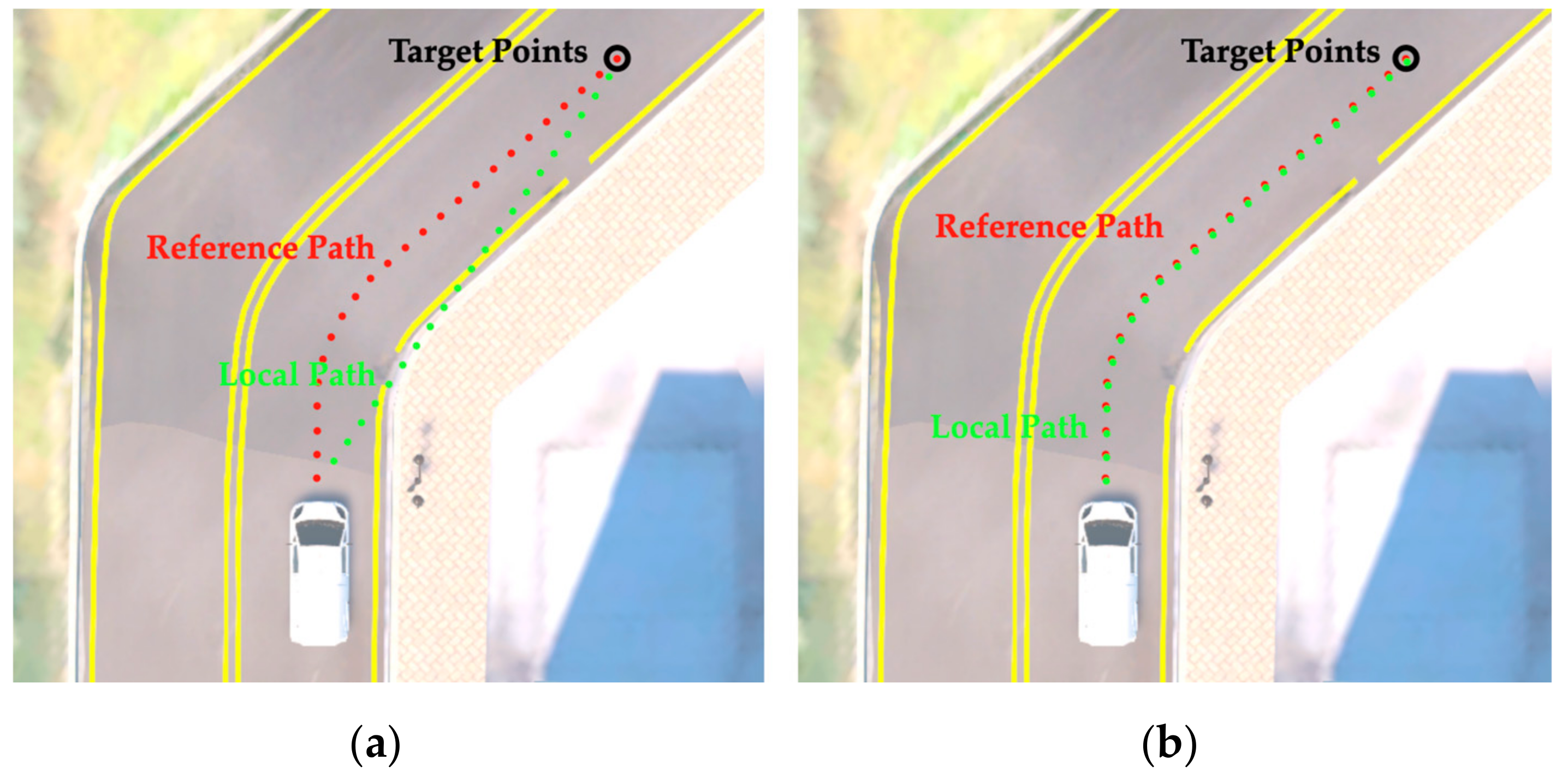
Our concept of local path planning is static object avoidance. When our delivery vehicle faces illegal parking vehicles, it has a negative effect on the service time if the delivery vehicle waits for evasive action. For safety, path planning should work well on any roads on a campus, such as straight roads, curved roads, and corner roads. In general, general path planning algorithms set one arrival point to reach and search for the shortest path. However, this method is not useful for autonomous driving vehicles in real-world scenarios. In addition, an autonomous driving vehicle has to generate the shortest path by considering road constraints. For example, a problem happens when a vehicle is driving on curved/corner roads. Assuming that an autonomous vehicle is on a high curved road, when the vehicle chooses a point to reach, the path planner creates a penetrated path into the side of the lane if the point is far away, as shown in
Figure 1.
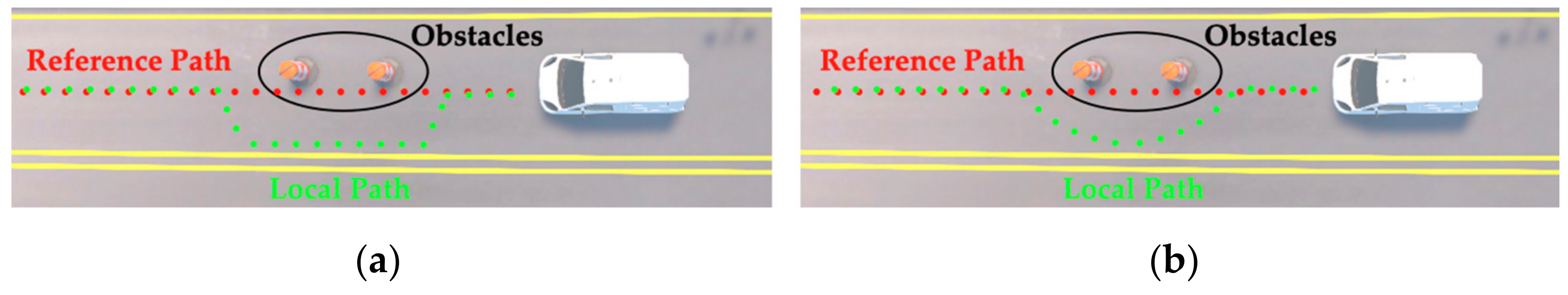
This algorithm should consider vehicle dynamics to avoid collisions resulting from the local path. The autonomous driving vehicle has a limited steering angle. If the local path curves sharply, the autonomous driving vehicle cannot trace this accurately. This is shown in
Figure 2. The vehicle in
Figure 2a does not consider the steer angle limit and the vehicle in
Figure 2b does.
4. Traditional Algorithm Analysis
4.1. A* Algoirthm
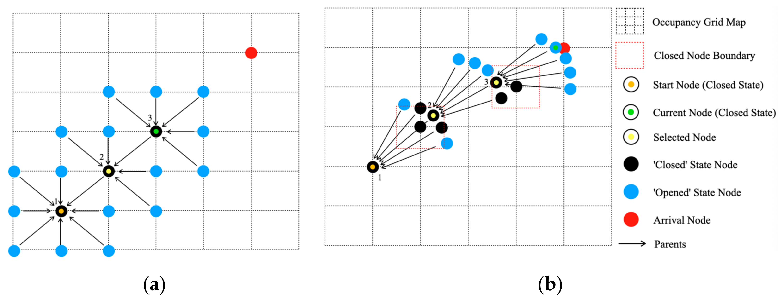
To handle path planning problems in a campus environment, the graph search algorithm was analyzed. The A* algorithm, which is representative among graph search algorithms, is a general method of finding the shortest path between a starting point and arrival point with guaranteed real-time performance. The principle of how to get the shortest path depended on the occupancy grid map and the distance cost. Each of the nodes had one state, namely ‘Opened’, ‘Closed’, or ‘Non’. At first, only the start node’s state is ‘Opened’. Another node is the state of ‘Non’, and based on the distance cost that is calculated by the Euclidean distance between the start node, the current node, and the arrival node, the low-cost node among the ‘Opened’ options is selected. By using this principle, the A* algorithm finds the shortest path; as shown in
Figure 3a.
However, the traditional A* algorithm is not suitable for a real vehicle environment. The path’s route points are generated at intervals of 45 degrees since these points are proliferated on a discrete occupancy grid map (
Figure 3a). It is therefore unsuitable for autonomous driving vehicles since the path angle of A* could be outside the allowable steering angle of 30 degrees. To solve these problems, Hybrid A* [
18,
19,
20] was proposed, which was applied in the DARPA Urban Challenge [
21], a competitive contest of autonomous driving vehicles. This algorithm has the same principle as A* except for the propagation type. A* use a discrete propagation method while Hybrid A* uses a continuous propagation method (
Figure 3b). Since Hybrid A* uses continuous propagation, it can consider vehicle kinematic models. Therefore, the path angle generated from Hybrid A* satisfies the allowable steering angle of vehicles.
However, it is difficult for the Hybrid A* algorithm to consider the constraints. For example, in the vehicle road environment, a mobile robot should observe lane information; the A* algorithm, however, could not obey these constraints.
4.2. Artificial Potential Field
The route of a local path based on APF is determined by the cost of the virtual force field. The virtual force field consists of attractive and repulsive forces. Each of these has the ability to pull or push propagated path points. The repulsive force is granted to obstacles that should be evaded. The path is generated by propagating from the start point to the target point under the influence of a virtual force. The general virtual force equation is denoted as follows:
where
,
, and
are the force fields. Each is a total virtual force field, attractive force field, and repulsive force field.
,
, and
are the propagating point, target point, and obstacle point, respectively, and consist of a two-dimensional
position.
is the distance between the propagating point and obstacle. If
is larger than
, the repulsive force is not affected by the propagated point.
This algorithm is very efficient as a solution to complex situations since multiple obstacle data points are formed as a function. However, it has a critical problem in that it does not converge on the goal point. When attractive force and repulsive force get a same cost value, the sum of these is set as 0 and the route reaches the local optima.
5. Proposed Path Planning Algorithm
To handle these campus path planning problems, multiple goal potential field Hybrid A* (MGPF-Hybrid A*) is proposed. This proposed algorithm is based on the Hybrid A* algorithm and the APF method. APF is applied to consider the road constraints and multiple obstacle avoidances and APF then replaces the Hybrid A*’s cost model, which is calculated by the Euclidean distance.
5.1. Introduction of Path Propagation Model
The propagation model of MGPF-Hybrid A* is similar to that of Hybrid A*. It has two node types; one is a grid map node (GMN) and another is a propagated node (PN). The two types of nodes are located in Cartesian coordinates consisting of . The GMN is allocated ‘Opened’ and ‘Closed’ states. When the proposed path planner is operated, the size of the GMN is assigned. The other node, named PN, is the candidate of the generated path. When we operate the proposed path planner, the number of nodes that are PNs increase step-by-step from the start node. If the PN reaches the end point of the given reference path, the traced organization of the final PN to the start node is the local path point of MGPF-Hybrid A*.
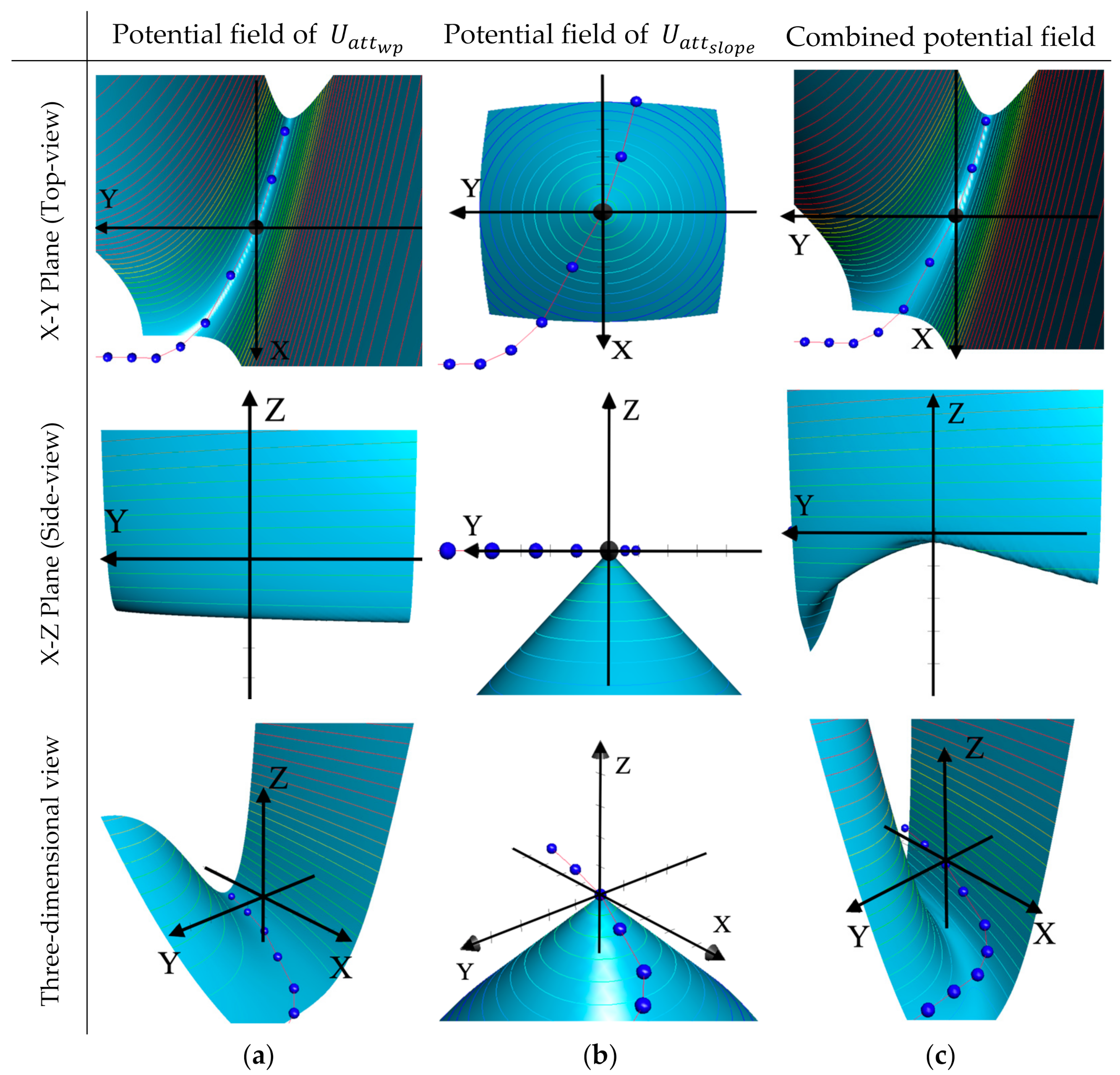
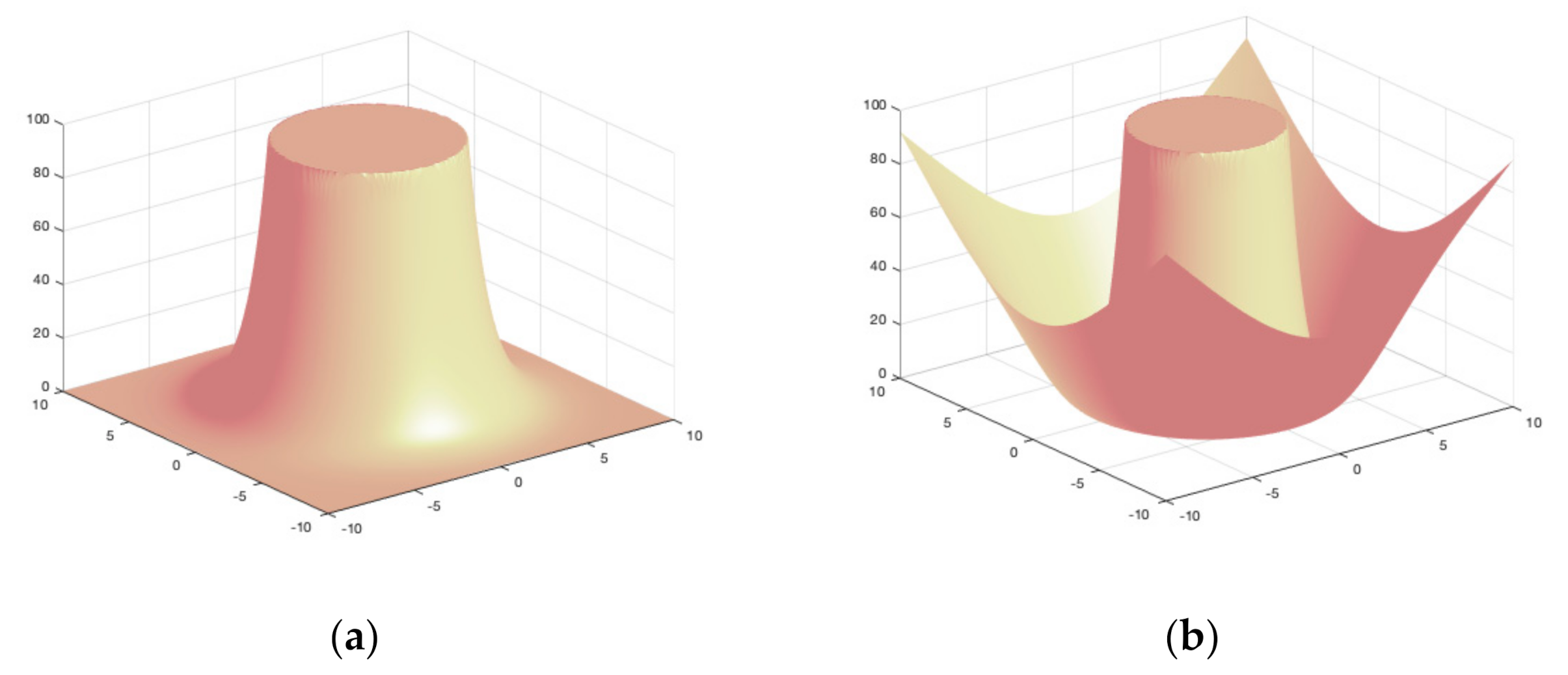
Since this is a step-by-step propagation, it is related to operating time. Assuming that it uses a tree model, in which the start node is the root node, and the target node is one of the branch nodes far from the root node, if the PNs behave like the breadth-first-search method, it takes a great deal of time to converge on the global optima. On the other hand, if the behavior is similar to that of the depth-first search method, and it selects the correct sub-tree direction, it will take a small amount of time. Therefore, to induce the second method, APF is applied. This APF generates a potential valley toward the reference path which the PN should follow. This valley indicates the correct sub-tree direction of the depth-first search method. The height caused by the valley indicates the cost. The closer to the valley, the smaller the cost, and the farther away from the valley, the larger the cost. If the valley pulls the PN, real-time performance will be guaranteed. The potential field depicting a valley is shown in
Figure 4a.
5.2. Artificial Potential Field Considering Road Constraints and Multiple Obstacles
To attract our micro-EV using reference path points, methods leveraging APF are proposed. The traditional attractive force considers only one goal point. On the other hand, our proposed algorithm could consider multiple goal points. In this paper, multiple goals indicate the reference path points. These reference path points are changed to a polynomial to facilitate calculations, as shown in Equation (6). Generally, the Clothoid curve model [
22] is applied in vehicle curve fitting. However, this model is generally applied to roads with a road speed of 60 km/h or greater is used. It is not acceptable for our campus environment. Therefore, the Bayesian curve fitting method [
23] is applied for curve fitting to this polynomial. To make the cost dimension
, the polynomial is squared. As a result, this form takes a three-dimensional Cartesian coordinate
, as shown in Equation (7) (
Figure 4a). The
and
denoted in Equation (7) represent the PN
points. In Equation (7), the PN points converge on the reference polynomial line, wherever it is located, since the cost value increases toward the far direction from the polynomial line region. The reference polynomial line is shown in
Figure 4 as a red line.
If there is no negative slope toward the far points from the start node, the PNs located on the low-cost valley will not propagate quickly toward the end of the valley, which affects real-time performance. Therefore, the farther away from the starting node, the lower the cost value should be, as shown in Equation (8). In addition, it takes a three-dimensional Cartesian coordinate
. This equation results in the potential field shown in
Figure 4b. The final attractive force results from the sum of Equations (7) and (8), as shown in
Figure 4c. The introduced equation is as follows:
Unlike the reference path points, the obstacles have a repulsive force [
24]. Additionally, the obstacles are handled in the discrete domain. The obstacles are dots on a grid map at intervals of 10 cm. Each dot point is expressed in the form of an exponential function to reduce the field region’s effect that is farther away and improve the closer field region’s effect. This method is beneficial compared to traditional repulsive force functions since the effect region is calculated with only one parameter,
, without a threshold value (
Figure 5).
The equation of this repulsive force is Equation (9).
and
are the positions of obstacles. The equation is as follows:
The entire proposed cost of the potential field is denoted as the sum of attractive and repulsive forces and is shown in Equation (10). This entire potential field function is applied to the Hybrid A*’s cost model.
There are hyper-parameters, , in Equations (7)–(9). These are related to the algorithm performance. is related to the gradient of the potential field, . If is high, the shape of will be sharpened. On the other hand, is related to real-time performance and if has a high value, it converges quickly toward the global optima. These are related to the gradient of the potential field. The larger the gradient toward the end of the multiple goals, the better the real-time performance. However, excessive gradient increase for rapid convergence causes the collapse of the potential fields. and are the 6-order and 1-order equations, respectively. Therefore, in a general situation, the differential value of is larger than . However, if we set a high , the result is reversed. In the combined potential field of and , the effect of will be weak while the effect of will be improved. This collapsed potential field is not able to generate a proper path. Therefore, appropriate and are required. is associated with the size of the region needed to avoid obstacles. If the value of is large, the avoidance path for the obstacle will be created further away from the obstacle. On the other hand, if the value is small, a path will be created with a small distance from the obstacle, resulting in a collision.
6. Performance Evaluation on Simulator
6.1. Simulator for Evaluation
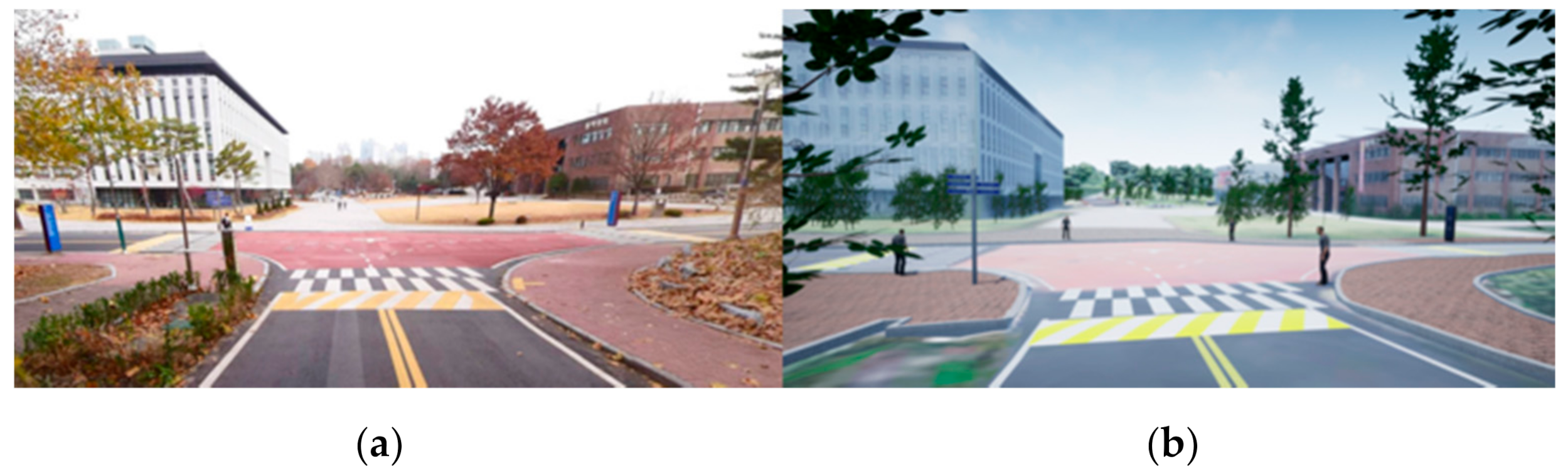
The MORAI simulator [
25], which is similar to real-world conditions, is used to evaluate our urban-based path planning. This simulator mimics the environment at the Chungbuk National University campus. An image is depicted in
Figure 6. The MORAI simulator was built to study autonomous driving vehicles; and adults, children, sedans, SUVs, and trucks can be included in the simulation environment. In addition, various sensors, such as cameras, LiDAR [
26], GNSS [
26,
27], and IMU [
26], which mimic autonomous vehicle’s real sensors, can be installed. Moreover, the simulator has a high degree of freedom. For example, our autonomous vehicle in the simulation can be controlled using a keyboard. Likewise, for the vehicle to be automatically controlled, the ROS protocol can be used [
28]. In this study, a micro-EV installed on MORAI was controlled using the ROS protocol.
6.2. Autonomous Systems for Evaluation
To operate our urban-based path planning algorithm, the autonomous system operating in a micro-EV was implemented. The systems are described as follows.
6.2.1. Software Architecture
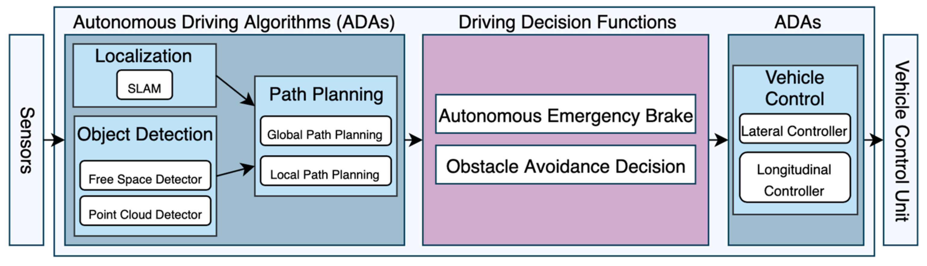
A pipeline of autonomous driving systems, constructed to evaluate path planning, is shown in
Figure 7. The proposed path planning is the local path planning inside part of the autonomous driving algorithm. This architecture can be divided into the following parts: autonomous driving algorithms and driving decision functions. The autonomous driving algorithms are designed to generate the data needed for general autonomous driving. Furthermore, the driving decision functions aims to determine whether micro-EV emergency braking behavior or avoiding actions occur. The details are depicted in the next section.
6.2.2. Localization Module
Simultaneous localization and mapping (SLAM) [
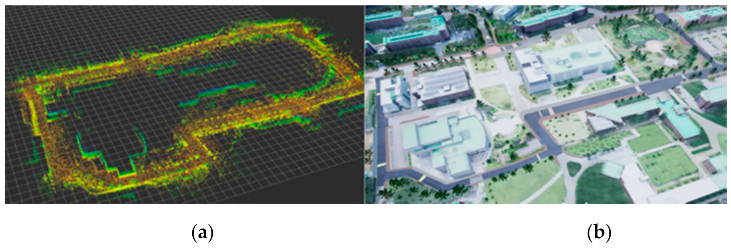
29], which utilizes a point clouds matching methods based on 3D LiDAR, was used. The GNSS was used to locate the initial position of the micro-EV based on SLAM. The way SLAM estimates localization is by assuming that the point clouds from LiDAR have accurate distance information. By projecting the point clouds acquired from real-time LiDAR on the stored reference map constructed using point clouds, accurate localization information is available. To build a point cloud reference map in an outdoor environment, the Graph SLAM [
30] and G-ICP [
30] methods are applied. After that, an interactive algorithm [
30] is applied to increase the accuracy of the point cloud reference map. The resulting reference map is shown in
Figure 8. The output data of this SLAM consisted of x, y orientation. In this study, when the micro-EV was driving, the localization accuracy was lower than 10 cm.
6.2.3. Object Detection Module
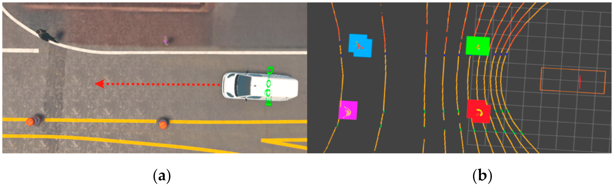
A rule-based LiDAR sensor algorithm was utilized to recognize obstacles. The data in the three-dimensional space are projected into a two-dimensional (x, y) plane and then detected through clustering tasks. The details are given in [
31]. The result of this method is shown in
Figure 9.
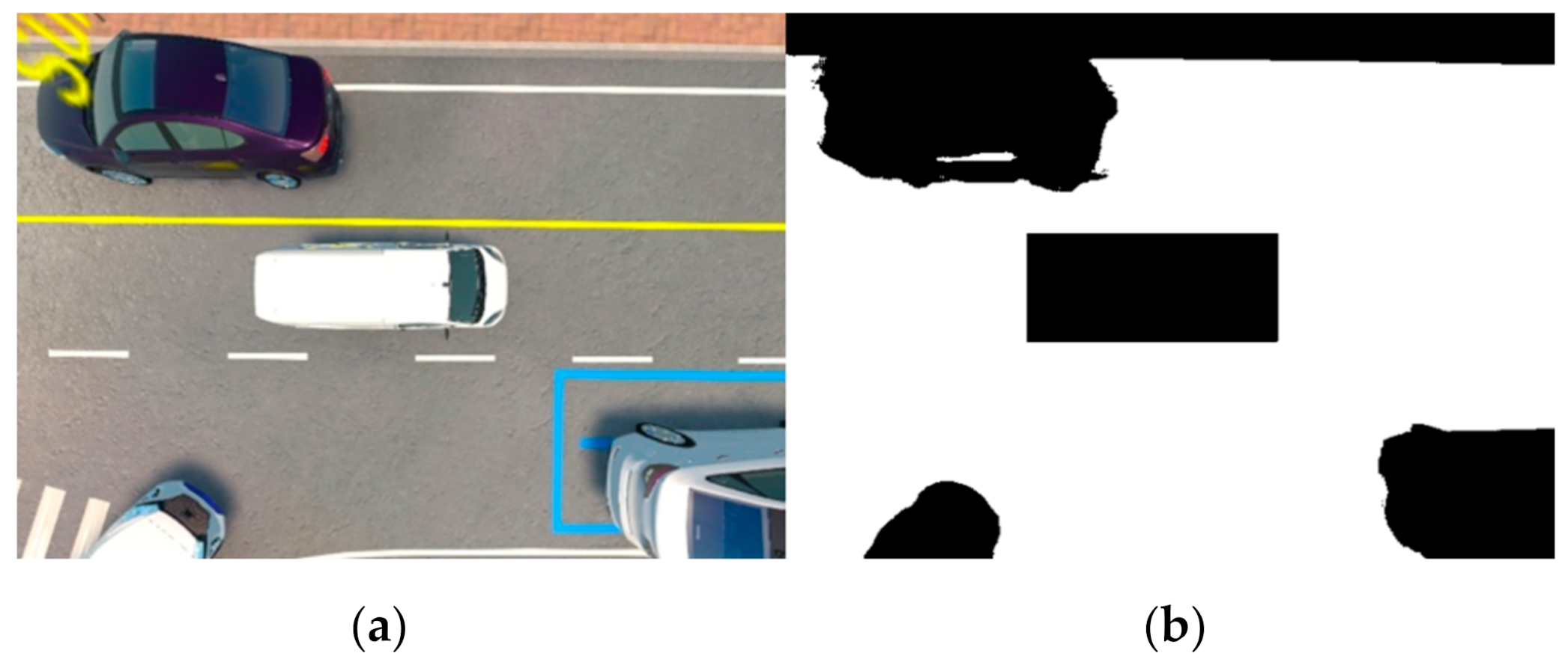
To cover the blind spot of LiDAR, a free space detection (FSD) algorithm was implemented based on AVM camera images [
32]. Since the object avoidance algorithm has to react immediately to avoid collisions, the FSD algorithm should be operated in real-time. In addition, it should obtain the accuracy distance. Therefore, ESPNet [
33], a learning-based algorithm to detect free space regions based on AVM camera images, was utilized. The result of this method is shown in
Figure 10.
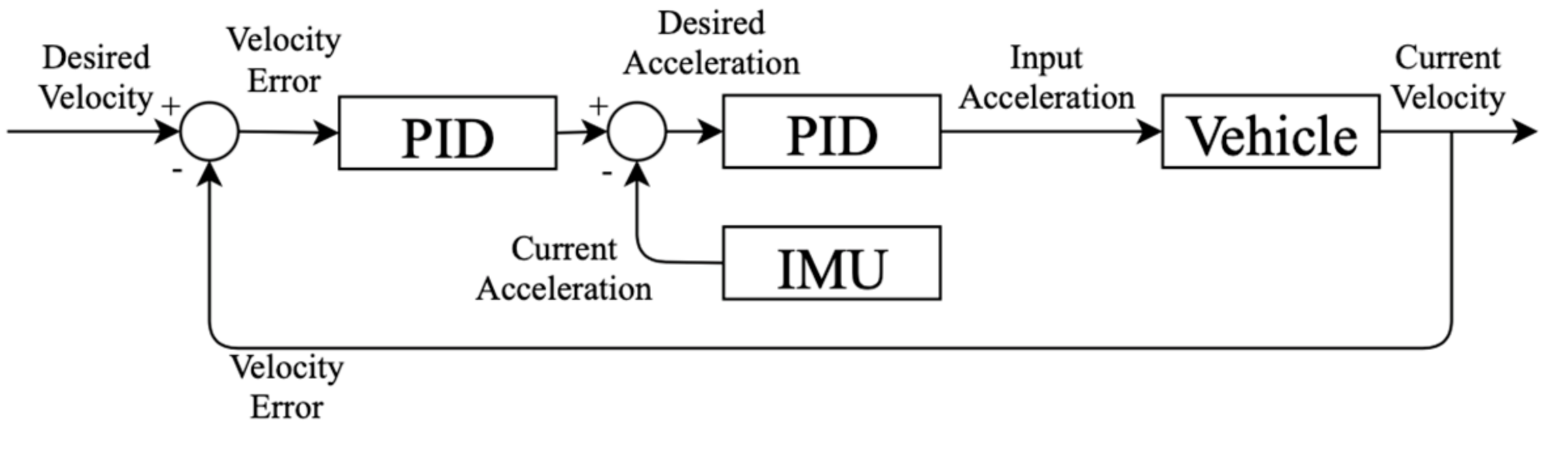
6.2.4. Path Following Module
For longitudinal control, a proportional–integral–differential (PID) controller is used. To get a robust behavior for sloped roads, the
X-axis acceleration value resulting from IMU was used and is shown in
Figure 11. For lateral control, a pure pursuit controller [
21,
34] was used. This algorithm is widely used for lateral control of vehicles below 40 km/h.
6.3. Performance of Path Planning
6.3.1. Path Accuracy Performance Measure
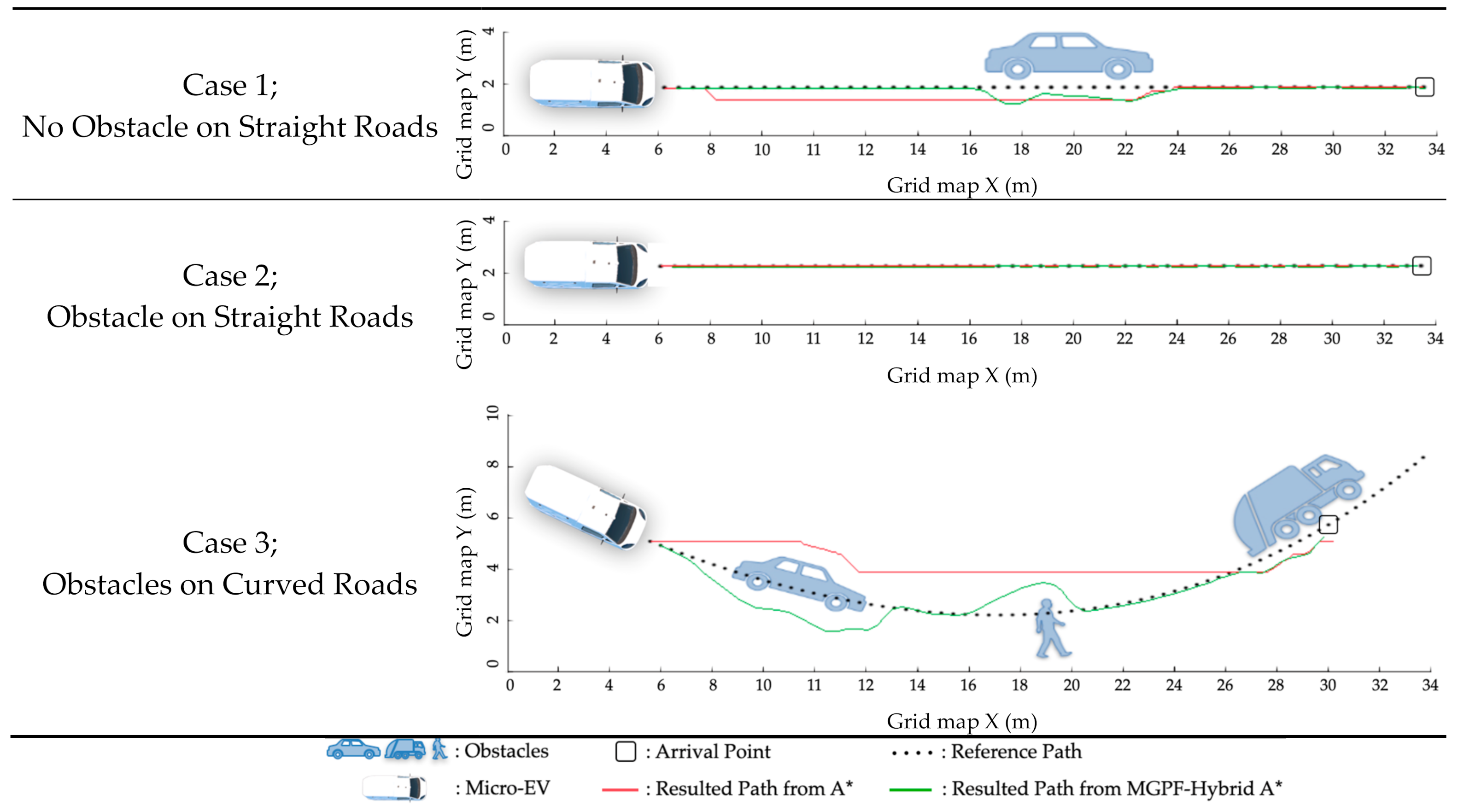
The MGPF-Hybrid A* algorithm is evaluated compared with A* in an environment of straight roads, straight roads with obstacles, and curved roads with obstacles. In this performance evaluation, an autonomous driving system is not applied. This measure simply evaluates the performance of the algorithm itself considering the obstacles without considering of the path-following performance. Moreover, since the input environment toward the proposed algorithm is the same as the output of the autonomous driving system, this evaluation is meaningful. The created path from the proposed MGPF-Hybrid A* is shown in
Figure 12. Moreover, all the scenarios are shown in
Figure 12, separated as cases 1, 2, and 3. The results of local path planning for each of the algorithms are drawn in the figures as green lines. Case 1 in
Figure 12 denotes a similar performance for the generated local path between A* and MGPF-Hybrid A*. However, there are performance gaps for path generating, as shown in case 2 of
Figure 12. MGPF-Hybrid A* has a better performance for following reference path points. A* unnecessarily changed the following path quickly. On the other hand, the MGPF-Hybrid A* performs a suitable collision-free operation. The ability to follow multiple goals is evident, as shown in case 3 of
Figure 12. A* does not consider the multiple goals. Therefore, on curved roads, A* disregards the reference path points. This could cause lane penetration when an autonomous vehicle is operated on a real road. On the other hand, the MGPF-Hybrid A* successfully follows multiple goals. In addition, since MGPF-Hybrid A* considers the vehicle steering model, the generated route is smoother than A*. The parameters of the MGPF-Hybrid used are,
. How to determine these parameters is introduced in the following sections.
The numerical evaluation of
Figure 12 is shown in
Table 1. The table denotes the error consisting of the distance gap between the generated path and the reference path by using the root mean square (RMS). The errors were calculated every 1-m interval. In case 1 which set as a straight path, the RMS of the A* algorithm was better than the proposed algorithm. However, the value does not make much of a difference for the autonomous driving environment. In cases 2 and 3, where obstacles and curve situations are considered, the proposed algorithm significantly outperforms the A* algorithm in regards to RMS values.
Except for the RMS values, the shortest path distance and the farthest path distance from the reference path were evaluated; the unit was meters. In
Table 1, each of these are denoted as D-Min and D-Max. In all situations, in cases 1, 2, and 3, the D-Min values are lower than 10 cm. This means that the algorithms, A* and MGPF-Hybrid A*, successfully converged on the reference path. The D-Max values of A* and MGPF-Hybrid A* in cases 1 and 2 were also similar, while the values in case 3 showed that the value of MGPF-Hybrid A* was lower than that of regular A*.
As a result of this evaluation, the proposed MGPF-Hybrid A* converged successfully on the reference path and it showed superior performance regarding multiple obstacles and curved road environments compared to the regular A* algorithm.
6.3.2. Real-Time Performance Measure
MGPF-Hybrid A* should satisfy real-time performance in order to operate under driving conditions. The real-time frequency should faster than 100 ms as was proven in [
35]. The factors which affected the real-time performance of MGPF-Hybrid A* were parameters
,
, and the numbers of obstacles projected on the occupancy grid map, ‘nObstacles’. Unlike the performance measure of path accuracy, real-time performance was evaluated on a MORAI simulator with an autonomous driving system.
and
were simulated by varying each value to find the optimal values and, the uncontrollable parameter, ‘nObstacles’, was also simulated by varying the number of points to prove real-time performance. In our environment, the occupancy grid map had a size of 200 × 400 cm, which consists of 10 × 10 cm pieces. On this grid map, the obstacle points were mapped and simulated. In the general scenario, the number of points was set to 200, and in the complex environment scenario, the number of points was set to 1400. The value of 1400 was the result of the arbitrary installation of many obstacles, surrounding the micro-EV, in the simulator. The experimental data are shown in
Table 2,
Table 3,
Table 4 and
Table 5.
Table 2 shows the results simulated on straight roads without obstacles, straight roads with obstacles, and curved roads with obstacles. Experiments mentioned in
Table 3,
Table 4 and
Table 5 were on curved roads, which is the result of the lowest performance measure of
Table 2. Good performance measure was obtained when the
and
set as 0.5 and 0.3, respectively. In addition, when the non-controllable parameter ‘nObstacles’ was set to the worst-case scenario value of 1400, it had an operating speed of 51.84 ms. The operating time, 51.84 ms, was lower than the required operating time of 100 ms, which means that the proposed algorithm could prove real-time performance using mathematical inductive methods. This performance results were obtained using the following hardware specifications: CPU i7-7700HQ 2.80GHz, RAM 16GB, and GPU NVIDIA GTX 1060 6GB.
6.3.3. Performance Evaluation on Campus Driving Situation Related to Hazard Scenarios
In this section, the path planning algorithm performance considering obstacles, pedestrians, and vehicles is evaluated. For all collision scenarios that could occur in our campus, hazardous scenarios that have critical damage for the micro-EV and pedestrians are sorted. The hazardous scenarios were obtained by manually driving the micro-EV around the real CBNU campus. Moreover, for high evaluation reliability, the Euro NCAP [
36] and ISO22737 r14.0 [
37] were referenced. For these scenarios, the path planner would design a proper path and vehicle control commands. The seven hazardous scenarios for possible collision risk situations in the campus environment were prepared. In all the scenarios, the micro-EV sequentially followed several behavior steps to evaluate the path planning algorithm operating in the autonomous systems:
When the micro-EV meets obstacles, the autonomous emergency brake system should be activated.
The micro-EV should determine whether the obstacle avoidance system should activate.
If the obstacle avoidance system is activated, the micro-EV should evade the obstacles in a collision-free operation. On the other hand, if the obstacle avoidance system is not an activated, the micro-EV should be placed in a state of braking.
If the micro-EV evades the obstacles, the obstacle avoidance system is deactivated. When the micro-EV meets obstacles, steps 1–4 are repeated.
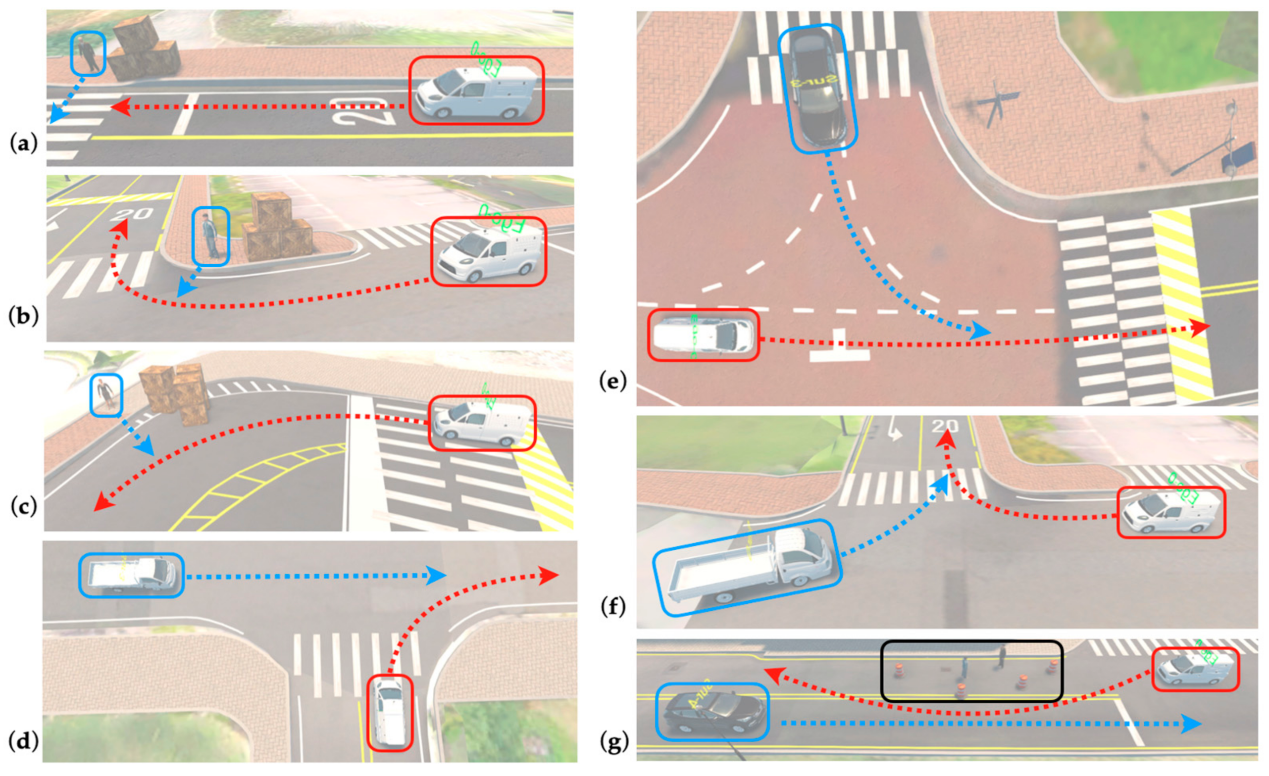
The seven hazardous scenarios prepared for evaluation are shown in
Figure 13. In this figure, the micro-EV is marked in red, the dynamic obstacles are marked in blue, and the static obstacles are marked in black. For each scenario, objects colored in red and blue move in the direction of their arrows. A detailed description of the scenarios is as follows:
For (a), this is a scenario in which pedestrians jump onto the road from a blind spot when the micro-EV is driving on a straight road. The pedestrians are set to move at 10 km/h and the pedestrians enter the roadway at a distance of 1.5 m from the front bumper of the micro-EV. The pedestrian’s cut-in scenario repeats four times to see whether the micro-EV could generate a proper local path after the pedestrians disappear.
For (b), this is the same as (a) except with the road shape changed from straight to a right curve. This cut-in scenario of pedestrians repeats five times to see whether the micro-EV performs the behavior of avoidance or not.
For (c), this is the same as (a) except with the road shape changed from straight to a left curve. This cut-in scenario of pedestrians repeats four times to see whether the micro-EV performs the behavior of avoidance or not.
For (d), this is a scenario in which obstacle vehicles, which drive on a straight road cut into the route of the micro-EV when the micro-EV turns right. The obstacle vehicles are set to move at 40 km/h. The number of obstacle vehicles is nine.
For (e), this is the same as (d) except that the obstacle vehicles and the micro-EV are opposite. There are four obstacle vehicles.
For (f), this is the same as (d) except that the obstacle vehicles turn left. There are four obstacle vehicles.
For (g), this is a scenario in which the micro-EV meets static obstacles on the road while the obstacle vehicles are moving in the side lane in which the micro-EV should drive when the obstacle avoidance system is activated. The obstacle vehicles are set to move at 40 km/h, and the number of the obstacle vehicles is five. During the time when the obstacle vehicles pass, the obstacle avoidance system is not be activated. After this, the micro-EV activates the obstacle avoidance system, offering collision-free operation.
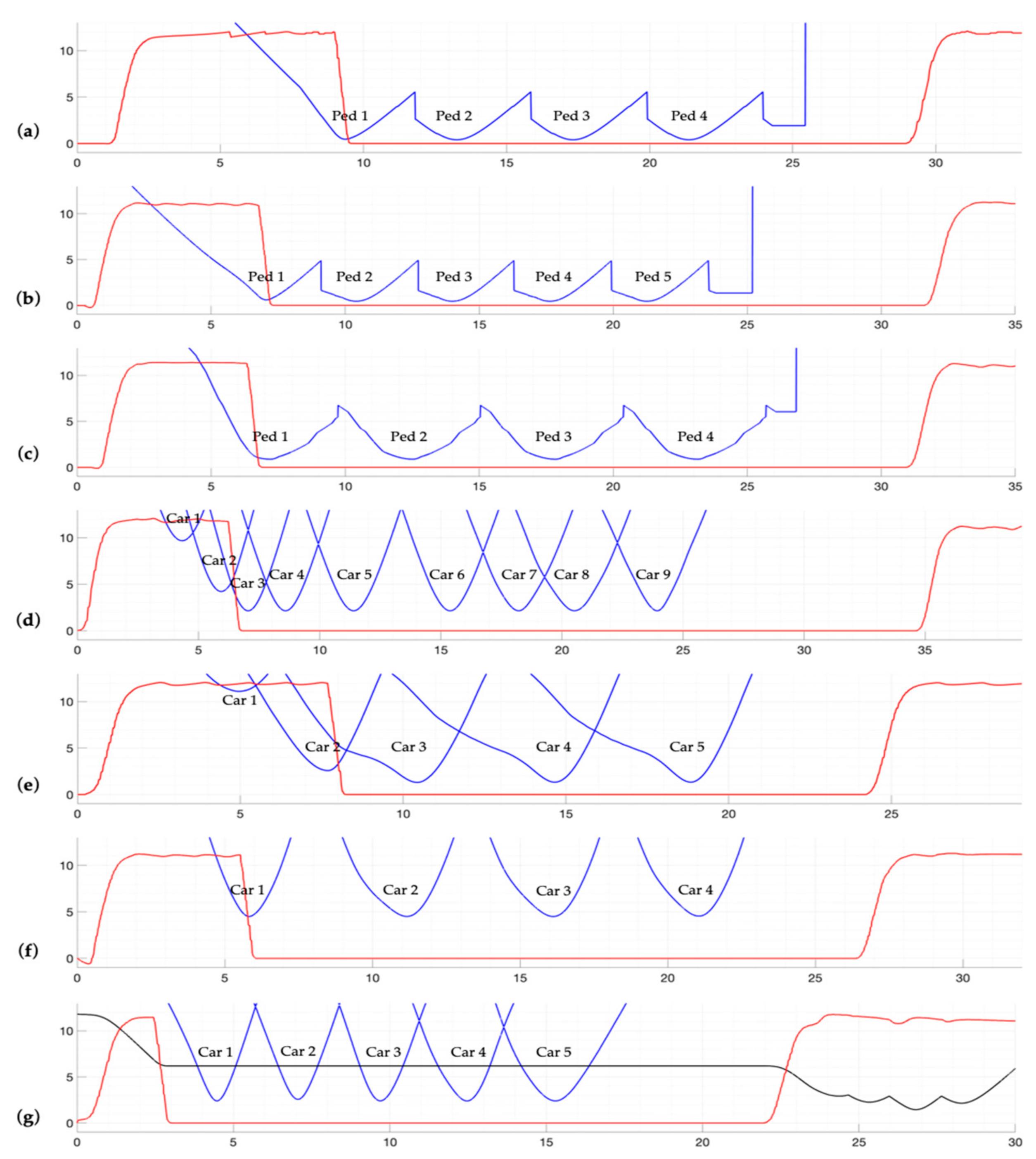
In these hazardous environments, the performance of path planning in the multiple-obstacle environment is evaluated. The results are shown in
Figure 14. In this figure, each sub-item, (a)–(f), corresponds to the sub-item of
Figure 13. The red-colored lines denote the speed of the micro-EV. The blue-colored lines denote a distance between the dynamic obstacles and the micro-EV. The black-colored lines denote a distance between the static obstacles and the micro-EV. For all situations, there was no collision, which was confirmed from blue and black lines. After the braking period, the micro-EV accelerated toward the generated path as confirmed by the red lines. During this acceleration, there were also no collisions related to obstacles. Based on these facts, we confirm that our proposed urban-based path planning algorithm is applicable for a complex campus environment.
7. Discussion
The research environment, CBNU campus, includes various obstacles, such as illegally parked cars, pedestrians, as well as road constraints. Moreover, the autonomous vehicles, the micro-EV, operated on the roads that had a high velocity greater than 5 m/s. Therefore, to guarantee the safety of the path generation, three requirement, obstacles, road constraints, and real-time performance, should be considered.
The Hybrid A* algorithm propagates the candidate path points in a continuous region, not in the discrete region used in A*. Moreover, it guarantees real-time performance and the shortest path generation. Therefore, it is studied broadly in the study of vehicle path planning. However, it is hard to consider the constraints since the cost model of Hybrid A* applies Euclidean distances. The artificial potential field, which mimics the concept of a gravitational field, has outstanding real-time performance, as does Hybrid A*. Moreover, the approach that formulates the attractive and repulsive forces simplifies various surrounding obstacles and road constraints. However, depending on the shape of the potential field, it could converge on the local optima instead of the global optima. This means that the generated path evades obstacles successfully, but could not converge on the desired reference path. Therefore, in the worst case, the generated path could penetrate side lanes, which should not be allowed.
This paper combines each of the advantages related to the Hybrid A* and artificial potential field methods. The combined algorithm has a real-time performance and guarantees the shortest path, obeying the road constraints, which were difficult to consider when we applied Hybrid A*. Additionally, the local optima problem, in which the PN could not converge to the target points, caused by the artificial potential field is solved by Hybrid A* since Hybrid A* does not revisit pre-visited nodes. Additionally, the Hybrid A*’s constraints consider the problem offset using an artificial potential field.
8. Conclusions and Future Work
In this paper, an urban-based path planning algorithm suitable for campus-environment autonomous driving vehicles is proposed. The path planning algorithm applied to the campus environment, MGPF-Hybrid A*, was proposed to ensure collision-free driving by considering road constraints and multiple obstacles. To consider campus-road constraints, the proposed algorithm used reference path points that considered road lanes. The reference path points are rebuilt as a polynomial equation. This approach solves the lane departure problem. The path polynomial equation and two-dimension obstacle data are applied to the artificial potential field to create attractive and repulsive forces that control the path points that can be generated by the proposed path planning algorithm. If the attractive force is high, it pulls toward the generated path. Otherwise, if the repulsive force is high, it pushes away from the generated path. To evaluate our urban-based path planning algorithm, the MORAI simulator, which mimics the campus of Chungbuk National University, is used. Moreover, to evaluate a real-world environment, autonomous driving algorithms, such as vehicle localization, object recognition, and vehicle control, are implemented. These are applied to the micro electric vehicle that exists within the MORAI simulator. In this simulation, our urban-based path planning algorithm successfully maintains road constraints and avoids multiple obstacles. Although the proposed algorithm is evaluated in a simulated environment, it is also tested on a real road of the CBNU campus using a micro-EV as an autonomous vehicle delivery service. The proposed algorithm could be used to determine a proper solution to static obstacles, which can be used for autonomous vehicle delivery services on a campus, but it does not have a flexible a path and lacks the same decision-making as a human driving. Therefore, further research will be conducted to reduce the burden on the decision logic of the autonomous vehicle driving system through path planning and which behavior decisions are considered for dynamic obstacles.
Author Contributions
Conceptualization, C.P.; methodology, C.P.; validation, C.P.; writing—original draft preparation, C.P.; writing—review and editing, S.-C.K.; supervision, S.-C.K.; funding acquisition, S.-C.K. All authors have read and agreed to the published version of the manuscript.
Funding
This research was supported by the MSIT (Ministry of Science and ICT), Korea, under the Grand Information Technology Research Center support, program(IITP-2021-2020-0-01462) supervised by the IITP(Institute for Information & communications Technology Planning & Evaluation).
Institutional Review Board Statement
Not applicable.
Informed Consent Statement
Not applicable.
Data Availability Statement
Conflicts of Interest
The authors declare no conflict of interest.
References
- Baemin Dilly. Available online: https://robot.baemin.com (accessed on 26 April 2021).
- Hart, P.E.; Nilsson, N.J.; Raphael, B. A Formal Basis for the Heuristic Determination of Minimum Cost Paths. IEEE Trans. Syst. Sci. Cybern. 1968, 4, 100–107. [Google Scholar] [CrossRef]
- Koenig, S.; Likhachev, M. Fast replanning for navigation in unknown terrain. IEEE Trans. Robot. 2005, 21, 354–363. [Google Scholar] [CrossRef]
- Karaman, S.; Frazzoli, E. Sampling-based algorithms for optimal motion planning. Int. J. Robot. Res. 2011, 30, 846–894. [Google Scholar] [CrossRef]
- Ghosh, D.; Nandakumar, G.; Narayanan, K.; Honkote, V.; Sharama, S. Kinematic Constraints Based Bi-directional RRT (KB-RRT) with Parameterized Trajectories for Robot Path Planning in Cluttered Environment. In Proceedings of the 2019 International Conference on Robotics and Automation, Montreal, QC, Canada, 20–24 May 2019. [Google Scholar]
- Lu, L.; Gong, D. Robot Path Planning in Unknown Environments Using Particle Swarm Optimization. In Proceedings of the International Conference on Natural Computation, Jinan, China, 18–20 October 2008; pp. 422–426. [Google Scholar]
- Adamu, P.; Jegede, J.T.; Okagbue, H.; Oguntunde, P. Shortest Path Planning Algorithm—A Particle Swarm Optimization (PSO) Approach. In Proceedings of the World Congress on Engineering, San Francisco, CA, USA, 23–25 October 2018. [Google Scholar]
- Bounini, F.; Gingras, D.; Pollart, H.; Gruyer, D. Modified Artificial Potential Field Method for Online Path Planning Applications. In Proceedings of the IEEE Intelligent Vehicles Symposium, Los Angeles, CA, USA, 11–14 June 2017. [Google Scholar]
- Wu, S.; Du, Y.; Zhang, Y. Mobile Robot Path Planning Based on a Generalized Wavefront Algorithm. Math. Probl. Eng. 2020, 2020, 1–12. [Google Scholar] [CrossRef]
- Katrakazas, C.; Quddus, M.; Chen, W.-H.; Deka, L. Real-time motion planning methods for autonomous on-road driving: State-of-the-art and future research directions. Transp. Res. Part C Emerg. Technol. 2015, 60, 416–442. [Google Scholar] [CrossRef]
- Stahl, T.; Wischnewski, A.; Betz, J.; Lienkamp, M. Multilayer Graph-Based Trajectory Planning for Race Vehicles in Dynamic Scenarios. In Proceedings of the IEEE Intelligent Transportation Systems Conference, Paris, France, 9–12 June 2019. [Google Scholar]
- Werling, M.; Ziegler, J.; Kammel, S.; Thrun, S. Optimal trajectory generation for dynamic street scenarios in a Frenét Frame. In Proceedings of the 2010 IEEE International Conference on Robotics and Automation, Anchorage, AK, USA, 3–7 May 2010; pp. 987–993. [Google Scholar] [CrossRef]
- Karaman, S.; Frazzoli, E. Optimal kinodynamic motion planning using incremental sampling-based methods. In Proceedings of the IEEE Conference on Decision and Control, San Diego, CA, USA, 13–15 December 2010; pp. 7681–7768. [Google Scholar]
- Hu, X.; Chen, L.; Tang, B.; Cao, D.; He, H. Dynamic path planning for autonomous driving on various roads with avoidance of static and moving obstacles. Mech. Syst. Signal Process. 2018, 100, 482–500. [Google Scholar] [CrossRef]
- Zhang, Y.; Chen, H.; Waslander, S.L.; Gong, J.; Xiong, G.; Yang, T.; Liu, K. Hybrid Trajectory Planning for Autonomous Driving in Highly Constrained Environments. IEEE Access 2018, 6, 32800–32819. [Google Scholar] [CrossRef]
- Rasekhipour, Y.; Khajepour, A.; Chen, S.-K.; Litkouhi, B. A Potential Field-Based Model Predictive Path-Planning Controller for Autonomous Road Vehicles. IEEE Trans. Intell. Transp. Syst. 2016, 18, 1255–1267. [Google Scholar] [CrossRef]
- Borrelli, F.; Falcone, P.; Keviczky, T.; Asgari, J.; Hrovat, D. MPC-based approach to active steering for autonomous vehicle systems. Int. J. Veh. Auton. Syst. 2005, 3, 265. [Google Scholar] [CrossRef]
- Montemerlo, M.; Becker, J.; Bhat, S.; Dahlkamp, H.; Dolgov, D.; Ettinger, S.; Haehnel, D.; Hilden, T.; Hoffmann, G.; Huhnke, B.; et al. Junior: The Stanford entry in the Urban Challenge. J. Field Robot. 2008, 25, 569–597. [Google Scholar] [CrossRef]
- Petereit, J.; Emter, T.; Frey, C.W. Application of Hybrid A* to an Autonomous Mobile Robot for Path Planning in Unstructured Outdoor Environments. In Proceedings of the 7th German Conference on Robotics, Munich, Germany, 21–22 May 2012. [Google Scholar]
- Sedighi, S.; Nguyen, D.V.; Kuhnert, K.D. Guided Hybrid A-star Path Planning Algorithm for Valet Parking Applications. In Proceedings of the International Conference on Control, Automation and Robotics, Shenzhen, China, 19–21 July 2019. [Google Scholar]
- DARPA Grand Challenge. 2007. Available online: https://en.wikipedia.org/wiki/DARPA_Grand_ Challenge_(2007) (accessed on 26 April 2021).
- Baass, K.G. Use of Clothoid Templates in Highway Design. Transp. Assoc. Can. (TAC) 1984, 1–3, 47–52. [Google Scholar]
- Ravankar, A.; Ravankar, A.A.; Kobayashi, Y.; Hoshino, Y.; Peng, C.-C. Path Smoothing Techniques in Robot Navigation: State-of-the-Art, Current and Future Challenges. Sensors 2018, 18, 3170. [Google Scholar] [CrossRef] [PubMed]
- Glaser, S.; Vanholme, B.; Mammar, S.; Gruyer, D.; Nouveliere, L. Maneuver-Based Trajectory Planning for Highly Autonomous Vehicles on Real Road With Traffic and Driver Interaction. IEEE Trans. Intell. Transp. Syst. 2010, 11, 589–606. [Google Scholar] [CrossRef]
- Autonomous Driving Simulator, MORAI. Available online: https://www.morai.ai (accessed on 26 April 2021).
- Campbell, S.; Mahony, N.O.; Krapalcova, L.; Murphy, A.; Ryan, C. Sensor Technology in Autonomous Vehicles. In Proceedings of the IEEE Irish Signals and Systems Conference (ISSC), Belfast, UK, 21–22 June 2018. [Google Scholar]
- Rubinov, E.; Collier, P.; Fuller, S.; Seager, J. Review of GNSS Formats for Real-Time Positioning. PositionIT 2012, 27, 20–27. [Google Scholar]
- ROS. Available online: http://wiki.ros.org/Documentation (accessed on 26 April 2021).
- SLAM (Simultaneous Localization and Mapping). Available online: https://www.mathworks.com/discovery/slam.html (accessed on 26 April 2021).
- Koide, K.; Miura, J.; Menegatti, E. A PorTable 3D LIDAR-based System for Long-term and Wide-area People Behavior Measurement. Int. J. Adv. Robot. Syst. 2019, 16, 1–16. [Google Scholar] [CrossRef]
- Sualeh, M.; Kim, G.W. Dynamic Multi-LiDAR Based Multiple Object Detection and Tracking. Sensors 2019, 19, 1474. [Google Scholar] [CrossRef] [PubMed]
- De Silva, V.; Roche, J.; Kondoz, A. Robust Fusion of LiDAR and Wide-Angle Camera Data for Autonomous Mobile Robots. Sensors 2018, 18, 2730. [Google Scholar] [CrossRef] [PubMed]
- Mehta, S.; Rastegari, M.; Caspi, A.; Shapiro, L.; Hajishirzi, H. ESPnet: Efficient spatial pyramid of dilated convolutions for semantic segmentation. In Proceedings of the European Conference on Computer Vision (ECCV), Munich, Germany, 8–14 September 2018. [Google Scholar]
- Snider, J.M. Automatic Steering Methods for Autonomous Automobile Path Tracking; CMU-RI-TR-09-08; 2009. Available online: https://www.ri.cmu.edu/pub_files/2009/2/Automatic_Steering_Methods_for_Autonomous_Automobile_Path_Tracking.pdf (accessed on 26 April 2021).
- Broggi, A.; Medici, P.; Zani, P.; Coati, A.; Panciroli, M. Autonomous vehicles control in the VisLab Intercontinental Autonomous Challenge. Ann. Rev. Control 2012, 36, 161–171. [Google Scholar] [CrossRef]
- 2018 Automated Driving Tests. Available online: https://www.euroncap.com/en/vehicle-safety/safety-campaigns/2018-automated-driving-tests/ (accessed on 26 April 2021).
- Intelligent Transport Systems—Low-Speed Automated Driving (LSAD) Systems for Predefined routes—Performance Requirements, System Requirements and Performance Test Procedures. Available online: https://www.iso.org/obp/ui/#iso:std:iso:22737:dis:ed-1:v1:en (accessed on 26 April 2021).
Figure 1.
Wrong and correct case of local path planning; (a) the case in which the local route penetrates into the side of the road and (b) the case where the local route is generated correctly, following the reference path.
Figure 1.
Wrong and correct case of local path planning; (a) the case in which the local route penetrates into the side of the road and (b) the case where the local route is generated correctly, following the reference path.
Figure 2.
Problem of traditional local path planning; (a) the case in which the turning ratios of the vehicles are not considered and (b) the case in which the turning ratios of the vehicles are considered.
Figure 2.
Problem of traditional local path planning; (a) the case in which the turning ratios of the vehicles are not considered and (b) the case in which the turning ratios of the vehicles are considered.
Figure 3.
A comparison between regular A* and hybrid A*; (a) description of the A*’s node proliferation and (b) description of Hybrid A*’s node proliferation.
Figure 3.
A comparison between regular A* and hybrid A*; (a) description of the A*’s node proliferation and (b) description of Hybrid A*’s node proliferation.
Figure 4.
Potential field visualization drawn on three-dimensional Cartesian coordinates. The contour line denotes the height of the cost value. The blue circle denotes the reference path points. The red line, crossing the zero point, denotes the Bayesian polynomial calculated from the reference path points. The zero point (0, 0, 0) mean the center of gravity of the micro-EV. (a) Denotes Equation (6). The potential valley is shown through the x-y plane; (b) denotes Equation (7). The slope is shown through the x-z plane; (c) denotes the sum of Equation (6).
Figure 5.
The comparison of exponential functions of repulsive potential forces (a) and traditional repulsive potential fields (b). (a) No need to set threshold value and (b) should consider the distance threshold to remove the unintended potential force.
Figure 5.
The comparison of exponential functions of repulsive potential forces (a) and traditional repulsive potential fields (b). (a) No need to set threshold value and (b) should consider the distance threshold to remove the unintended potential force.
Figure 6.
Image similarity comparison between the real and virtual scenes. (a) Real scene and (b) virtual scene.
Figure 6.
Image similarity comparison between the real and virtual scenes. (a) Real scene and (b) virtual scene.
Figure 7.
Block diagram of the software algorithm architecture.
Figure 7.
Block diagram of the software algorithm architecture.
Figure 8.
(a) Point cloud reference map and (b) the environment of the Chungbuk National University, built in the MORAI simulator.
Figure 8.
(a) Point cloud reference map and (b) the environment of the Chungbuk National University, built in the MORAI simulator.
Figure 9.
Result of object detection based on LiDAR tested on a simulator: (a) Obstacle environment of simulator; and (b) the image displaying detected obstacles on the RVIZ tools. The detected obstacles are denoted as big boxes and the small lines refer to the 3D point clouds.
Figure 9.
Result of object detection based on LiDAR tested on a simulator: (a) Obstacle environment of simulator; and (b) the image displaying detected obstacles on the RVIZ tools. The detected obstacles are denoted as big boxes and the small lines refer to the 3D point clouds.
Figure 10.
Result of FSD based on AVM camera tested in a simulator: (a) input images; (b) the binarized result image. The black area means non-crossable obstacles.
Figure 10.
Result of FSD based on AVM camera tested in a simulator: (a) input images; (b) the binarized result image. The black area means non-crossable obstacles.
Figure 11.
Process flow of the vehicle longitudinal controller.
Figure 11.
Process flow of the vehicle longitudinal controller.
Figure 12.
Performance evaluation of A* and MGPF-Hybrid A*. The generated paths are drawn on a grid map.
Figure 12.
Performance evaluation of A* and MGPF-Hybrid A*. The generated paths are drawn on a grid map.
Figure 13.
The hazardous scenarios: (a–c) these are regarded as moving pedestrians; (d–g) these are regarded as moving vehicles.
Figure 13.
The hazardous scenarios: (a–c) these are regarded as moving pedestrians; (d–g) these are regarded as moving vehicles.
Figure 14.
The performance result for each hazardous scenario: (a–c) The results are regarded as moving pedestrians; (d–g) The results are regarded as moving vehicles. The X-axis means period of time. For the blue/black lines, the Y-axis means distance error denoted as meters between the micro-EV and obstacles. For the red lines, the Y-axis means current longitudinal speed in km/h.
Table 1.
Performance measures of A* and MGPF-Hybrid A*.
Table 1.
Performance measures of A* and MGPF-Hybrid A*.
| Each Scenario of Figure 12 | Regular A* | MGPF-Hybrid A* |
|---|
| Error | RMS | D-Min | D-Max | RMS | D-Min | D-Max |
| Case 1 | 0.0067 | 0.0001 | 0.0225 | 0.0112 | 0.0058 | 0.0210 |
| Case 2 | 0.7196 | 0.0001 | 1.0010 | 0.5493 | 0.0006 | 0.9449 |
| Case 3 | 2.9597 | 0.0021 | 4.6010 | 1.8369 | 0.0033 | 3.0450 |
Table 2.
Performance measure for real time; state of = 0.5, = 0.3, length 100 m, and nObstacles 400.
Table 2.
Performance measure for real time; state of = 0.5, = 0.3, length 100 m, and nObstacles 400.
| | Straight Road without Obstacles | Straight Road | Curved Road |
|---|
| Running Time (ms) | 3.79 | 6.99 | 21.36 |
Table 3.
Performance measure for real time; state of curved road, = 0.3, length 100 m, and nObstacles 400.
Table 3.
Performance measure for real time; state of curved road, = 0.3, length 100 m, and nObstacles 400.
| 0.5 | 0.7 | 1.0 |
|---|
| Running Time (ms) | 21.36 | 29.38 | 114.22 |
Table 4.
Performance measure for real time; state of curved road, = 0.5, length 100m, and nObstacles 400.
Table 4.
Performance measure for real time; state of curved road, = 0.5, length 100m, and nObstacles 400.
| 0.3 | 0.2 | 0.1 |
|---|
| Running Time (ms) | 21.36 | 47.73 | 627.03 |
Table 5.
Performance measure for real time; state of curved road, = 0.5, = 0.3, and length 100 m.
Table 5.
Performance measure for real time; state of curved road, = 0.5, = 0.3, and length 100 m.
| nObstacles | 400 | 800 | 1400 |
|---|
| Running Time (ms) | 21.36 | 29.95 | 51.84 |
| Publisher’s Note: MDPI stays neutral with regard to jurisdictional claims in published maps and institutional affiliations. |
© 2021 by the authors. Licensee MDPI, Basel, Switzerland. This article is an open access article distributed under the terms and conditions of the Creative Commons Attribution (CC BY) license (https://creativecommons.org/licenses/by/4.0/).


