Abstract
The article presents the results of multivariate calculations for the levitation metal melting system. The research had two main goals. The first goal of the multivariate calculations was to find the relationship between the basic electrical and geometric parameters of the selected calculation model and the maximum electromagnetic buoyancy force and the maximum power dissipated in the charge. The second goal was to find quasi-optimal conditions for levitation. The choice of the model with the highest melting efficiency is very important because electromagnetic levitation is essentially a low-efficiency process. Despite the low efficiency of this method, it is worth dealing with it because is one of the few methods that allow melting and obtaining alloys of refractory reactive metals. The research was limited to the analysis of the electromagnetic field modeled three-dimensionally. From among of 245 variants considered in the article, the most promising one was selected characterized by the highest efficiency. This variant will be a starting point for further work with the use of optimization methods.
1. Introduction
A heat treatment, and in particular the melting of highly reactive metals, is quite a serious technological challenge. There are several techniques for melting and creating alloys of reactive metals: arc melting, melting in a cold crucible furnace and levitation melting. Only the latter technique provides a natural full separation of the melted material from the furnace components that may contaminate the metal bath. Unfortunately, levitation melting is the most difficult to implement in practice [1]. It is characterized by low energy efficiency and high sensitivity to the parameters, construction of the melting device and the properties of the melted material [2,3]. To obtain maximum melting efficiency, the parameters of the melting system should be properly selected for the melted material and its volume [3,4,5,6,7,8]. It seems that the best solution would be to apply optimization to the design. Unfortunately, for a complete computational model including electromagnetic field, temperature field and flow field analysis, it is a difficult problem due to the complexity of the model and the long computation time [9,10].
The paper is a preliminary stage of research covering the construction of a computational model. It concerns the electromagnetic field modeled in three geometric dimensions and multi-variant analysis of different shapes of the inductor coil, different supply frequencies and different positions of the batch inside the inductor. The purpose of the multi-variant calculation was to check the computational model and find the most advantageous configurations of the levitation melting system. The issue of melting reactive metals is important, inter alia, because titanium and its alloys are increasingly used in various technological aspects like the aviation, space technology and in medical prosthetics. Unfortunately, titanium also has a very high melting point and a high reactivity. Electromagnetic levitation has also other application areas, such as actuation [11], transportation [12], electromagnetic bearing [13,14] and others [15,16,17].
In the literature, the problem of levitation melting has been present for quite a long time [5,18,19,20,21]. Initially, it concerned practically implemented inductor systems, because analytical computational methods allowed for modelling of such a system in a very simplified manner. The use of numerical methods significantly accelerated and widened the scope of research [22] from simplified models covering only the analysis of the electromagnetic field, through models including coupled analysis of the electromagnetic field and temperature, to models taking into account the coupling of electromagnetic field temperature and fluid dynamics fields. Initially, of course, the models were created as two-dimensional models, followed by the advancement as 3D models. However, the necessity to couple the three types of field to this day causes computational problems to conduct a numerical analysis of electromagnetic levitation. Currently, progress is made especially in the area of flow modeling, where Reynolds Averaged Navier–Stokes Models are increasingly replaced by Scale Resolving Simulation models (e.g., LES).
The complete levitation melting computational model includes the coupled analysis of the electromagnetic field, temperature and fluid dynamics fields. As a result of the effect of the electromagnetic field inside the batch, eddy currents are induced, which causes the appearance of electrodynamic forces and heating of the batch. If the direction and magnitude of the electrodynamic forces are “correct”, the batch may begin to levitate. As the temperature of the batch changes, its material properties also change, which causes a change in the levitation conditions; if the batch melts, its shape changes, which also changes the calculation model. A sketch of the relationship between the fields is presented in Figure 1.
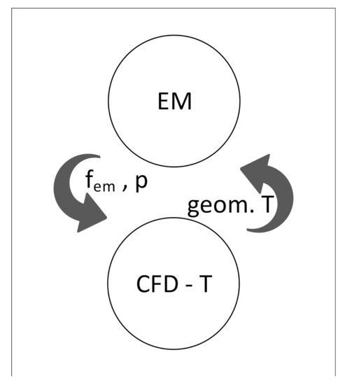
Figure 1.
Relationship between physical fields during levitation melting. stands for the electromagnetic field; refers to the fluid dynamics and temperature calculation; is the geometry and temperature change, after calculation; is the electromagnetic force density, and p corresponds to volumetric power value obtained from field calculation.
As can be seen from the above description, the phenomenon of metal melting using electromagnetic levitation is very complex. The most obvious way of the electromagnetic levitation modelling is to compute the electromagnetic field, temperature and the flow field in the time domain, but the time step needed to calculate the EM field is much shorter than the time step needed to analyze the other fields. Performing calculations with such a short time step leads to a very large computational effort and a long calculation time.
To avoid this, hybrid calculation models are often used, in which the analysis of the electromagnetic field is conducted as quasi-static (harmonic) and the analysis of the temperature field and flow field is already performed in the time domain. Such a calculation scheme allows one to extend the time step but leads to problems with the modeling of non-linearity of the electromagnetic field (B = f (H)). Moreover, it makes it necessary to achieve convergence between the electromagnetic field and the temperature and flow field models iteratively. In future research, we will use a hybrid model for calculations, and therefore, in this publication, the analysis of the electromagnetic field is conducted in the same way as the harmonic field.
Aim or the Research and Contribution of the Paper
The aim of the research presented in the paper is a survey of conditions and physical parameters, which results in the batch levitation and the maximization of power efficiency of the melting for a selected class of inductors. For this purpose, the coil geometry, current frequency and batch position are considered to be variable, while the basic dimensions of the coil remain invariable. The main constraint of optimization is the possibility of reaching an equilibrium state by batch inside the coil that allows it to levitate, which is crucial in this metal melting methodology.
This research should be treated as an introduction to future multi-parameter optimization. The results obtained provide valuable insight about shape of the cost function (the power efficiency), which is handy for selecting the suitable optimization algorithm. They also allow for rough formulation of constraints imposed on parameters values that satisfy the occurrence of levitation condition. Finally, the best results will constitute the starting point for more thorough optimization in the next stage of research.
2. Materials and Methods
Due to the relatively high cost of implementation, which requires selecting of an inductor, current and batch parameters, numerical modeling, and simulation of electromagnetic field using FEM is a popular approach to prototyping of the solution [23]. There is a large variety of software to calculate the FEM model. There are commercial products like Ansys, Flux, Comsol or Solidworks, but there are also open-source solutions such as gmsh with GetDP, GetFem++ or Agros with Artap [24,25].
2.1. Software and Hardware Platform
Due to the earlier experience of the researchers, the geometry was implemented in gmsh. This is a three-dimensional finite element mesh generator with four main modules: geometry, mesh, solver, and post-processing. Furthermore, it is distributed under the terms of the GNU General Public License [26]. In order to simulate the discussed metal melting process, the GetDP program was selected. It is an FEM solver where mixed elements to discretize the Rham-type complexes are used [27]. To perform multivariant calculation, a python script was used to generate each model geometry in gmsh language and to process simulation results.
The main simulation was calculated on a server equipped with 2 Intel Xeon 2.40 GHz processors and 40 GB RAM. A total number of 245 simulations, which took approximately 400 h of calculations, were conducted.
2.2. Electrical and Geometrical Parameters
For the computational experiment, the classical model of a conical levitation inductor featuring one turn of coil rewound, was adopted. The shape of the inductor is based on the actual application of the inductor hence it lacks symmetry. Furthermore, the geometry of the inductor is compatible with the power source available to researchers which is important due to future validation.
The top and bottom of most wires are connected to a power source. The second notable part of the coil is located just under the top wire, and it contains an inflexion within the contour, which allows it to change the current direction. The cross-section of the 3D model considered in the paper is presented in Figure 2.

Figure 2.
The cross-section of the inductor.
The exact parameters of the model are:
- the total height of coil —0.06 m
- the coil wire radius —0.003 m,
- the vertical distance between neighborhood wire—0.002 m
- the batch radius —0.0025 m,
- the weight of the batch—0.000176715 kg,
- the radius of bottom wire —0.01 m,
- coil is made of copper,
- batch is made of aluminum,
- electrical conductivity of copper—6 · S/m,
- electrical conductivity of aluminum—3 · S/m,
- the current—100 A.
As the research are in the preliminary stage, the batch made of aluminum instead of titanium was assumed due to its low melting temperature and small weight. It is more suitable for the multivariate analysis of the electromagnetic levitation system, as it is easier to achieve both the levitation and melting. It is also a common practice shown in other research [28]. As mentioned, other parameters were variable. To be precise:
2.3. Calculation Model
As described above, the model was implemented in three-dimensional space. High-level tools dedicated to determine the coupling widening towards the top is not available in the program used. Therefore, coil geometry was manually designed. The wire leading from the power source was based on a straight line. Beyond it was where the wire began coiling, and each full turn of the wire was divided into 4 parts. All of them are based on circle functions with a different center position and a growing radius. The concept is shown in Figure 3. Before the last turn, a change in direction follows. Afterwards, the wire was linked back to the source of power by a straight line.
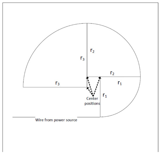
Figure 3.
The concept of coil geometry.
As is shown in Figure 4, the box shape of the surroundings was adopted. Its edges were almost two times longer than the inductor’s height. The batch inside the inductor was modeled as a ball. Although the simulation time of such a model is quite significant (approximately 1 to 1.5 h), it provides more credible results with comparison to the 2D coaxial model.
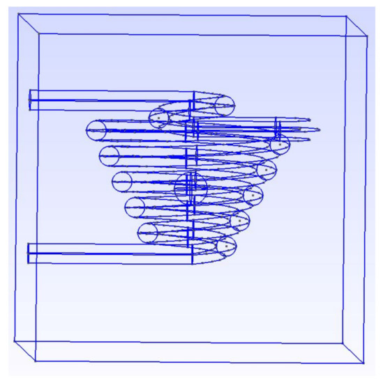
Figure 4.
Geometry model of inductor.
The distance between adjacent nodes of the Finite Elements Method (FEM) depends on the depth of penetration of the electromagnetic field (1) in the chosen material type. The tetrahedral finite element was used.
- —field penetration,
- —angular frequency,
- —conductivity,
- —magnetic permeability.
2.4. Mathematical Model of the Electromagnetic Field
Referring to previous points, the calculations were limited to the analysis of the electromagnetic field modeled in three-dimensional space. The analysis was carried out for the harmonic field, and the main results were represented as the volumetric density of the electrodynamic forces and the electrodynamic forces acting on the batch.
The analysis of the electromagnetic field was based on Equations (2) and (3). The value of the vector potential acquired from (2) and (3), and the magnetic induction B (4) and current density J (5) were calculated. Finally, the volumetric density of the electrodynamic forces (6) and the forces acting on the batch F (7) were obtained. Active power inducted in the electromagnetic field was based on (8).
where:
- —magnetic vector potential,
- —imaginary unit,
- —angular frequency,
- —conductivity,
- —magnetic permeability,
- —electric potential,
- —magnetic flux density,
- —current density,
- —electromagnetic force density,
- —electromagnetic force,
- —electromagnetic power.
3. Results
During the experiment, the following parameters were controlled: the ascending force , total power supplied to the system , power dissipated in the batch , which allows estimating the efficiency of the process, and the other forces acting on the batch. The names of axes and forces applied to the batch are shown in Figure 5.
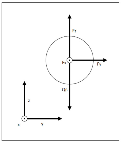
Figure 5.
The axes and forces applied to the batch. is ascending force, is gravity force, and and are horizontal force applied to the batch.
3.1. The Forces
The capability of levitation inside the inductor is a crucial matter in this case, and it is expressed in the difference between the and gravitational force acting on the batch shown in Figure 6. For the tested variant, the following remarks might be drawn:
- For each current, the frequency maximum of was achieved for = and = 0.035 m;
- The maximum of was obtained for f = 30 kHz;
- An increase in f causes an increase in (in the range f from 5 to 30 kHz);
- An increase in causes an decrease in (in the range from to );
- Every simulation performed for f = 5 kHz resulted in impossibility of batch levitation.
The absolute condition for achieving levitation is that the electromagnetic buoyancy force is in the the balance with gravitational force . From a theoretical point of view, for each inductor, there should be two points where this balance occurs [21]. In our experiment, both points were observed for a frequency of 30 kHz and an angle of .

Figure 6.
Difference between vertical components of the force and gravity applied to the batch in N for different values of the frequency , different positions of the batch and different values of the angle . Positive values, where levitation occurs, are marked by a dark blue color.
If the batch is knocked out above the top equilibrium point, the electromagnetic buoyancy force becomes lower than gravity force ; thus, the batch will start to descend. However, if the batch passes below this equilibrium point, the overcome , so the batch will be pushed back towards the top equilibrium. Therefore, the top equilibrium point should be considered as stable, which means that the batch should levitate in it during a melting process [3]. On the other hand, a different situation can be observed for a bottom equilibrium point. If the batch goes below this equilibrium point, the will be higher than , so it will pull the batch further down. Above the bottom equilibrium point, the batch is pushed up towards the top equilibrium point. This is why this bottom point should be considered an unstable one. Both equilibrium points (bottom and top) are shown in Figure 7d. The distance between those is correlated with , so it increases while grows.
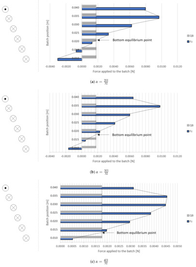
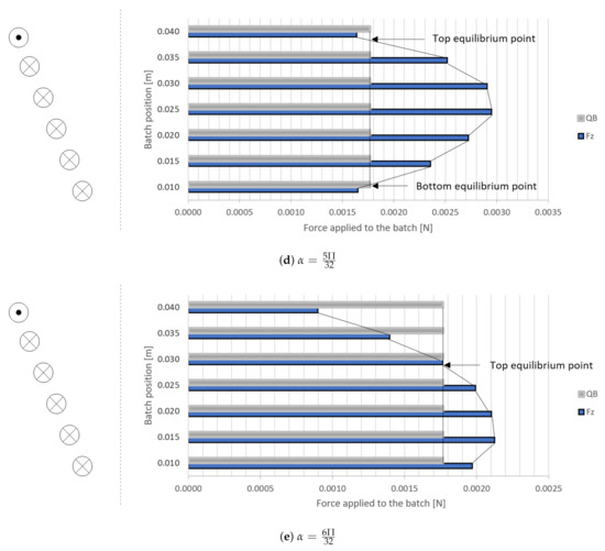
Figure 7.
The relationships between and for f = 30 kHz and different . On the left side of each table, a cross-section of the inductor is shown (according to Figure 2) to visualise the batch position.
The following observations were made:
- For = (Figure 7d), the value of resembles a square function with a negative slope. The batch is levitating near the top wire of the inductor.
- For more narrow angles from (Figure 7a–c), rises with as long as the position is below the = 0.35 m. This is a result of the fact that the wires are close to the batch, which increase , pushing the batch up. The top wire with opposite current slightly counteracts it, and the batch achieves a stable position above the top wire.
- For angle (Figure 7e), significantly decreases while rises. This is due to the fact that the top wire is too far away to have efficient impact on the batch. In this case the batch is levitating.
The values of the horizontal components of the force applied to the batch are negligibly small in comparison the to ; therefore their presentation was omitted in this paper. However, it is worth mentioning that those components are not equal to zero due to asymmetry of the model (wires leading to a power source and the inflexion in top wire). The horizontal forces are discussed further in Section 3.3.
3.2. Inducted and Supplied Power
The power inducted in the batch () is shown in Figure 8. It is directly proportional to f and counter-proportional to and . The magnitude of impact of all those variables on is similar. The maximum power inducted in the batch was obtained for f = 35 kHz, = and = 0.01 m.
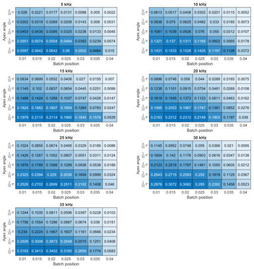
Figure 8.
Total power inducted on the batch W for different values of the frequency , different positions of the batch , and different values of the angle . The darker color corresponds to higher value.
In Figure 9, a total power supplied to the system () is presented. The angle and current frequency f have a most noticeable impact on , while the position of the batch seems to be less important. If the is smaller, the total length of wire is also shorter, which implicates a lower supplied, and higher f increases the power, while seems to have no significant impact on it. Although levitation does not occur, the maximum was achieved for f = 35 kHz, = .
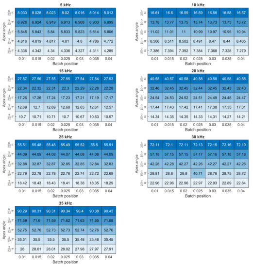
Figure 9.
Total power supplied to the coil W, for different values of the frequency , different positions of the batch , and different values of the angle . The darker color corresponds to higher value.
The power ratio (9) is shown in Figure 10. It is used to describe the efficiency of the melting process:
- For each f, the melting process was found to be more efficient if is low and the position of the batch is close to bottom wire.

Figure 10.
The efficiency for different values of the frequency , different positions of the batch , and different values of the angle . The darker color corresponds to higher value.
3.3. Selected Variant
To achieve a high economic result of the melting process, the highest possible power efficiency should be obtained, but only if the batch is in the upper equilibrium point. Due to fact that the parameters are isolated points, the highest that levitated was selected. Therefore, as the starting point for future optimisation, the variant f = 10 kHz, = , and = 0.03 m was selected as the most promising one.
For the selected variant, the stability analysis of the horizontal batch position was also performed. For the different , the calculation was conducted and is presented in Table 1. The horizontal forces ( and ) act in opposing direction to the horizontal displacement like in a pendulum.

Table 1.
Simulation results for various horizontal positions of the batch.
As a finial analysis, it must be verified if, for a selected variant, power efficiency is sufficient to melt the batch. The calculations were conducted according to Equations (10)–(12) for the initial temperature of 20 °C. The energy needed for the batch melting was obtained from (10).
where:
- is the energy needed to increase the temperature to melting temperature,
- is the latent heat energy.
- C is the specific heat capacity,
- m is the weight of the batch,
- is the difference between starting temperature and melting temperature.
- is the latent heat.
Heat losses during melting occur due to two main reasons: radiation and convection. Therefore, the calculations were divided into two parts. In the first, only radiation causing heat losses were taken under consideration, because in actual applications, melting of the batch was performed in a vacuum [29]. In the second part, these calculations were complemented by heat losses caused by convection. It has to be emphasized, that such calculations are very simplified. In reality, every alternation of the temperature modifies the batch properties and implies a requisite of recalculation of power inducted in the batch. This makes an iterative approach to EM-T calculations necessary (according to Figure 1).
The equation for the energy of heating and radiation cooling the batch is shown in (13).
where:
- is the energy in the batch in the time domain,
- is the energy inducted in the batch by electromagnetic field in the time domain,
- is the energy lost by radiation in the time domain.
The power inducted on the batch was calculated during simulation. Therefore, the energy to heat the batch could be calculated according to (14).
where:
- is the power inducted in the batch,
- t is the time.
The energy lost to radiation is calculated based on (15).
where:
- is the emissivity of chosen material type,
- is the Stefan–Boltzmann constant,
- is the current temperature of the batch,
- is the current temperature of surroundings,
- S is the surface of the batch.
If the heat losses caused by convection are taken into account, due to, e.g., lack of vacuum, those can be estimated according to:
where:
- is the energy lost by convection in the time domain.
The energy lost at convection is calculated based on (18).
where:
- is the heat transfer coefficient.
The final equation describing the energy requirement for melting the charge is given by the equation:
Based on equations from this subsection, the calculation was conducted for = 10 , = 0.01, and at the start, is equal to = 20 °C. The time step for the calculation was t = 1 s. According to Figure 8, the for the selected variant is 0.1197 W. The result is:
- if only radiation is considered, the temperature stabilized at 452 °C, which unfortunately was insufficient to achieve melting.
- if convection is also taken into account, it resulted in even lower temperature of 157 °C.
During a survey of possible variants, we considered the wide range of frequencies, so the current in simulations was set to a value that is achievable for all of them. Fortunately, the selected variant uses f = 10 kHz, which allowed us to increase the current value. For the higher current value, increased, and melting occurred. The calculations of energy for the follwing selected variantsleads to the results summarized in Table 2
- = 101.835 J,
- = 69.979 J,
Table 2.
Results of the simulation of the batch heating for the different current.
Table 2.
Results of the simulation of the batch heating for the different current.
| Current [A] | [W] | for Radiation [s] | for Radiation and Convection [s] |
|---|---|---|---|
| 200 | 0.6073 | 464 | did not occurs |
| 300 | 1.3665 | 149 | 239 |
| 500 | 3.7958 | 48 | 54 |
It must be mentioned that at this stage of the research, the parameters of the process are not yet fully optimized, so the melting is possible but the time is not relatively high.
4. Discussion
The presented experiment concerned multi-variant calculations for the levitation melting model of a certain class of the inductors. In the experiment, three parameters have been changed: half apex angle, current frequency, and the vertical position of the batch. Subsequently, the forces applied to the batch, the power inducted in the batch, and the power supplied to the inductor were controlled. Therefore observations were taken for the following:
- The maximum efficiency where levitation occurs is for f = 10 kHz, = and = 0.03 m. This variant was selected as most promising one for future optimisation.
- Vertical component () of the force applied to the batch achieves the maximum for f = 30 kHz, = and = 0.035 m.
- The highest efficiency was reached for f = 10 kHz, = , and = 0.015 m, even though the batch in this position did not levitate.
- The power inducted in the batch () is maximum for f = 35 kHz, = , and = 0.01 m; however, the batch did not levitate.
- The maximum of total power supplied to the system () was obtained for f = 35 kHz, = , and = 0.04 m. However, levitation did not occur.
- The melting of the batch for the selected variant was confirmed (for the increased inductor current).
Moreover, all results obtained during this experiment provided valuable information for subsequent stage of research, which is the optimization of the melting efficiency:
- The efficiency of the process (power ratio) will be used as the cost function in future optimization.
- According to results obtained for all considered variants, no local extrema were found in the solution space. Therefore, the classical local-search algorithms should be sufficient for conducting the future optimization.
- Furthermore, the hard condition of the batch levitation allows rough constraints to be applied to model parameters, reducing the size of the solution space. It was found that f must be greater than 5 kHz, and if it is equal or lower than
- −
- 15 kHz, the should be less than .
- −
- 10 kHz, the should be less than and the should be greater than 0.02 m.
- −
- 25 kHz, the should be greater than 0.01 m.
Future research will be conducted in a few ways. Firstly, the model will be confirmed in physical measurement. Furthermore, the simulation will be expanded for the batch position where stable equilibrium point occurs. Furthermore the optimisation of performance with parameters with the greatest potential will be commenced, and finally, the optimized physical inductor for metal melting process will be constructed.
Author Contributions
Conceptualization, R.P. and B.N.; methodology, B.N.; software, B.N.; formal analysis, R.P.; investigation, L.M.; resources, B.N.; writing—original draft preparation, B.N.; writing—review and editing, L.M. and R.P.; supervision, R.P. All authors have read and agreed to the published version of the manuscript.
Funding
This research was funded by Silesian University of Technology grant number BKM-776/RM4/2020; 11/040/BKM20/0019.
Institutional Review Board Statement
Not applicable.
Informed Consent Statement
Not applicable.
Data Availability Statement
https://github.com/bnycz/ElectromagneticLevitationBKM2020, accessed on 22 April 2021.
Conflicts of Interest
The authors declare no conflict of interest.
References
- Bojarevics, V.; Pericleous, K.; Cross, M. Modeling the dynamics of magnetic semilevitation melting. Metall. Mater. Trans. B 2000, 31, 179–189. [Google Scholar] [CrossRef]
- Brisley, W.; Thornton, B.S. Electromagnetic levitation calculations for axially symmetric systems. Br. J. Appl. Phys. 1963, 14, 682–686. [Google Scholar] [CrossRef]
- Yadav, S.; Verma, S.; Nagar, S. Optimized PID Controller for Magnetic Levitation System. IFAC-PapersOnLine 2016, 49, 778–782. [Google Scholar] [CrossRef]
- Spitans, S.; Baake, E.; Jakovics, A.; Franz, H. Numerical and experimental investigations of a large scale electromagnetic levitation melting of metals. In Proceedings of the 10-th PAMIR International Conference—Fundamental and Applied MHD, Cagliari, Italy, 20–24 June 2016. [Google Scholar]
- Okress, E.C.; Wroughton, D.M.; Comenetz, G.; Brace, P.H.; Kelly, J.C.R. Electromagnetic Levitation of Solid and Molten Metals. J. Appl. Phys. 1952, 23, 545–552. [Google Scholar] [CrossRef]
- Jahanshahi, S.; Jeffes, J. Design of coils for levitating droplets of metals with improved temperature control characteristics. Trans. Inst. Min. Metall. Sect. C Miner. Process. Extr. Metall. 1981, 90, C138–C141. [Google Scholar]
- Fromm, E.; Jehn, H. Electromagnetic forces and power absorption in levitation melting. Br. J. Appl. Phys. 1965, 16, 653–663. [Google Scholar] [CrossRef]
- Kermanpur, A.; Jafari, M.; Vaghayenegar, M. Electromagnetic-thermal coupled simulation of levitation melting of metals. J. Mater. Process. Technol. 2011, 211, 222–229. [Google Scholar] [CrossRef]
- Royer, Z.L.; Tackes, C.; LeSar, R.; Napolitano, R.E. Coil optimization for electromagnetic levitation using a genetic like algorithm. J. Appl. Phys. 2013, 113, 214901. [Google Scholar] [CrossRef]
- Roth, E.A.; Margerum, E.A.; Amick, J.A. Evaporation of Silicon and Germanium by rf Levitation. Rev. Sci. Instrum. 1962, 33, 686–687. [Google Scholar] [CrossRef]
- Rodrigues, C.; Dias, M.; Martins, L.; Silva, D.; Araújo, J.; Oliveira, J.; Pereira, A.; Ventura, J. A magnetically-activated thermal switch without moving parts. Energy Convers. Manag. 2019, 197, 111881. [Google Scholar] [CrossRef]
- Ye, L.; Liang, C.; Liu, Y.; Li, D.; Liu, Z. Performance analysis and test of a novel eddy-current braking & heating system for electric bus. Energy Convers. Manag. 2019, 183, 440–449. [Google Scholar]
- Chen, J.; Zhou, J.; Meng, G. Diamagnetic bearings for MEMS: Performance and stability analysis. Mech. Res. Commun. 2008, 35, 546–552. [Google Scholar] [CrossRef]
- Han, B.; Xue, Q.; Liu, X.; Wang, K. Multi-objective optimization design of a high-speed PM machine supported by magnetic bearings. Mech. Syst. Signal Process. 2017, 92, 349–363. [Google Scholar] [CrossRef]
- Hasanzadeh, S.; Vaez-Zadeh, S. Efficiency analysis of contactless electrical power transmission systems. Energy Convers. Manag. 2013, 65, 487–496. [Google Scholar] [CrossRef]
- Muley, P.D.; Henkel, C.; Abdollahi, K.K.; Marculescu, C.; Boldor, D. A critical comparison of pyrolysis of cellulose, lignin, and pine sawdust using an induction heating reactor. Energy Convers. Manag. 2016, 117, 273–280. [Google Scholar] [CrossRef]
- Han, W.; Chau, K.; Lam, W. All-utensil domestic induction heating system. Energy Convers. Manag. 2019, 195, 1035–1043. [Google Scholar] [CrossRef]
- Muck, O. German Patent No. 422004, October 30, 1923. [2] EC OKRESS, DM WROUGHTON, G. COMENETZ, PH BRACE, AND JCR KELLY, Electromagnetic levitation of solid and molten metals. J. Appl. Phys. 1952, 23, 545–552. [Google Scholar]
- Vail, L.W. Electromagnet. US Patent 2,400,869, 28 May 1946. [Google Scholar]
- Lovell, W.V. Electromagnetic Levitation Apparatus. US Patent 2,566,221, 28 August 1951. [Google Scholar]
- Peifer, W.A. Levitation melting……A Survey of the State-of-the-Art. JOM 1965, 17, 487–493. [Google Scholar] [CrossRef]
- Yadav, S.; Verma, S.; Nagar, S. Performance enhancement of magnetic levitation system using teaching learning based optimization. Alex. Eng. J. 2017, 57, 2427–2433. [Google Scholar] [CrossRef]
- Spitans, S.; Jakovičs, A.; Baake, E.; Nacke, B. Numerical Modeling of Free Surface Dynamics of Melt in an Alternate Electromagnetic Field: Part I. Implementation and Verification of Model. Metall. Mater. Trans. B 2013, 44, 593–605. [Google Scholar] [CrossRef]
- Karban, P.; Pánek, D.; Orosz, T.; Petrášová, I.; Doležel, I. FEM based robust design optimization with Agros and Ārtap. Comput. Math. Appl. 2021, 81, 618–633. [Google Scholar] [CrossRef]
- Pánek, D.; Karban, P.; Orosz, T.; Doležel, I. Comparison of simplified techniques for solving selected coupled electroheat problems. COMPEL Int. J. Comput. Math. Electr. Electron. Eng. 2020, 39, 220–230. [Google Scholar] [CrossRef]
- Geuzaine, C.; Remacle, J.F. Gmsh: A 3-D finite element mesh generator with built-in pre-and post-processing facilities. Int. J. Numer. Methods Eng. 2009, 79, 1309–1331. [Google Scholar] [CrossRef]
- Dular, P.; Geuzaine, C. GetDP Reference Manual: The Documentation for GetDP, a General Environment for the Treatment of Discrete Problems. Available online: http://getdp.info (accessed on 22 April 2021).
- Sassonker, I.; Kuperman, A. Electro-mechanical modeling of electromagnetic levitation melting system driven by a series resonant inverter with experimental validation. Energy Convers. Manag. 2020, 208, 112578. [Google Scholar] [CrossRef]
- Bomberger, H.; Froes, F. The melting of titanium. JOM 1984, 36, 39–47. [Google Scholar] [CrossRef]
Publisher’s Note: MDPI stays neutral with regard to jurisdictional claims in published maps and institutional affiliations. |
© 2021 by the authors. Licensee MDPI, Basel, Switzerland. This article is an open access article distributed under the terms and conditions of the Creative Commons Attribution (CC BY) license (https://creativecommons.org/licenses/by/4.0/).