Segmenting Star Images with Complex Backgrounds Based on Correlation between Objects and 1D Gaussian Morphology

Abstract

Space object recognition in high Earth orbits (between 2000 km and 36,000 km) is affected by moonlight and clouds, resulting in some bright or saturated image areas and uneven image backgrounds. It is difficult to separate dim objects from complex backgrounds with gray thresholding methods alone. In this paper, we present a segmentation method of star images with complex backgrounds based on correlation between space objects and one-dimensional (1D) Gaussian morphology, and the focus is shifted from gray thresholding to correlation thresholding. We build 1D Gaussian functions with five consecutive column data of an image as a group based on minimum mean square error rules, and the correlation coefficients between the column data and functions are used to extract objects and stars. Then, lateral correlation is repeated around the identified objects and stars to ensure their complete outlines, and false alarms are removed by setting two values, the standard deviation and the ratio of mean square error and variance. We analyze the selection process of each thresholding, and experimental results demonstrate that our proposed correlation segmentation method has obvious advantages in complex backgrounds, which is attractive for object detection and tracking on a cloudy and bright moonlit night.

1. Introduction

Thresholding segmentation [1] is an important process for space object recognition and extraction in star images. Stars and skylight backgrounds are separated by differences in grayscale, and segmentation thresholdings commonly used today are global thresholdings [2,3,4,5,6,7,8,9,10,11,12,13] and local thresholdings [14,15,16,17,18,19]. A global thresholding is to specify a unified thresholding for all pixels of an image, such as the Otsu method [2,3,4,5], maximum entropy method [6,7,8,9,10] and the minimum error thresholding method [11], which are only applicable to star images where the gray levels of objects and backgrounds are clearly distinguished. Local thresholding is selected according to features of different regions in star images, such as the Bernsen algorithm [14], Niblack algorithm [15,16], and layered detection strategy in irregularly sized subregions [19], and the selection of sub-blocks has a great impact on the results of image segmentation.

However, due to the influence of bright moonlight, thin clouds and vignetting effect of optical system, the local image backgrounds fluctuate greatly, and even many gray saturation regions appear. In this case, both types of thresholdings are hard to achieve good segmentation between complex backgrounds and dark objects. Gray thresholding segmentation ignores the imaging characteristics of space objects, whose energy distributions are presented as approximately symmetric Gaussian distributions and bright spots diffused to the surroundings [20,21,22,23]. However, 2D morphology of the bright spots is not always significant. On the one hand, for a dark target, its gray level is close to the intensity of the image background, and the 2D Gaussian morphology may be drowned by fluctuating backgrounds [24,25]. On the other hand, the objects and stars have a certain degree of elongation in the direction of relative motion within a few seconds of exposure time, and Gaussian features in the direction change. Therefore, we can only use 1D Gaussian morphology of object streaks in the vertical direction of relative motion. However, for a locally discontinuous dim object streak, its 1D morphology at every position is not consistent everywhere in complex backgrounds, and recognition effects are poor when point spread function (PSF) of the same amplitude is used to fit an object streak [26]. There are also some methods that apply deep learning to target detection [27,28], but a large amount of image data needs to be trained in the object detection process.

We aims at achieving star image segmentation by using the morphological characteristics of objects without relying on gray thresholding. Through the above analysis, it is known that 2D Gaussian function cannot accurately describe object streak morphology, and fitting a streak with 1D PSF with the same amplitude is not suitable for the poor background environment of star images. Accordingly, we introduce 1D Gaussian functions with different amplitudes for fitting each group of image data, utilizing the correlation between the image data and theoretical object models to respectively identify each group of data with Gaussian shapes in the streak area. In addition, we analyze the standard deviation and the ratio of mean square error and variance in each group of local image data, set reasonable thresholdings to separate objects from image background and remove false alarms. According to Gaussian morphology of objects and stars, our correlation segmentation method is independent of gray thresholding, which can flexibly use the morphological features of space objects, making the influence of complex backgrounds weaker and achieving better image segmentation.

2. Object Models and Algorithms

The CCD images taken by the Chinese Academy of Sciences Ground-based Optical Telescope with a 3.2° × 3.2° field of view, an 800 mm aperture and a 2″ angular resolutioncan be expressed as

I = bg + s + ob + n,

(1)

where I represents astronomical gray values of a CCD image, bg are deep space backgrounds, s are stars, ob are usually satellites and space debris, and n mainly includes Gaussian noise from the circuit and Poisson noise from dark current and background light.

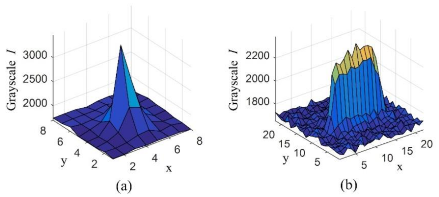
In different observation modes, objects or stars appear in different shapes on star images. When the telescope tracks the motion of stars, the stars are relatively stationary and appear as points, whereas the target appears as a streak. In this mode, the target streak needs to be extracted. On the contrary, when the telescope moves with the target, the target appears as a point and the stars appear as streaks. In this mode, the star streaks should be removed first. Therefore, the recognition of target streaks and star streaks is the focus of our work. We uniformly call such targets or stars with point shapes “point targets” and call those with long streak shapes “target streaks”, as shown in Figure 1. In the two observation modes, either the target or the stars are stationary relative to the star image. Therefore, the direction of the streaks is consistent with the direction of relative motion, and the streaks are straight.

The length of the streak is related to the target velocity relative to the stars and exposure time. We can appropriately increase exposure time to make the dark target brighter and easier to identify. However, with the increase of exposure time, the bright stars become saturated and the bright spots spread to a very large area around, which affects target recognition. Therefore, exposure time should be adjusted dynamically according to the use requirements and weather conditions, and for observing high-orbit space objects, usually exposure time is at second level. We take various noises, influence factors and deep space backgrounds together as undulating image backgrounds. In addition, we first rotate star images according to streak parameters and adjust the direction of the streaks to horizontal (the X-axis direction of the image is horizontal, and the Y-axis direction of the image is vertical). On this basis, we select 1D Gaussian function to lengthways fit them.

$${\tilde{y}}_k=BG+A\exp (\frac{-x_k{}^2}{2{\sigma }^2})$$

(2)

where ${\tilde{y}}_k$ are object gray values of the constructed model, BG are local image backgrounds, A is the object amplitude above the local background intensity, σ² is the variance of the Gaussian function, and $x_k$ are image ordinates. In order to ensure that the model can fit the image data better, mean square error should be minimized.

$$f\left(x_k;{\sigma }^2\right)=\frac{1}{n}{\displaystyle \sum _k^n{\left({\tilde{y}}_k-y_k\right)}^2}\to \min$$

(3)

where f is the mean square error function, and $y_k$ are observed object gray values. We find ${\sigma }_0^2$ when f is the minimum value, and the Gaussian function with ${\sigma }_0^2$ is the optimal fitting model for the group of data. The derivative of f is calculated as

$$\frac{A}{{\sigma }^4}{\displaystyle \sum _k^n\left(A{x}_k{}^2\exp \left(\frac{-x_k{}^2}{{\sigma }^2}\right)-\left(y_k-BG\right)x_k{}^2\exp \left(\frac{-x_k{}^2}{2{\sigma }^2}\right)\right)}\to 0$$

(4)

The pixel numbers occupied by dim objects in star images are different and unstable [29]. For star images taken by our wide field telescope, dim objects or stars usually occupy several pixels, and the bright stars usually occupy more pixels. Of course, the object size on the images is determined by telescope configuration and parameter setting, but it does not affect the extraction of column data with Gaussian form, and five continuous values can reflect the change trend of Gaussian morphology. If more data are selected, the computational complexity increases and overfitting occurs easily. Therefore, we select five consecutive pixels in a column to fit a Gaussian model at a time in the regions of interest or in the entire star image and take the center of the Gaussian model as the zero point, so the coordinates are

$$x_0{}^2=0,x_1{}^2=x_{-1}{}^2=1,x_2{}^2=x_{-2}{}^2=4$$

(5)

In addition, we set a parameter t = exp{−1/(2σ²)}, and Equation (4) is rewritten as

$$8A{t}^7-4\hspace{0.17em}\left(y_2+y_{-2}-2BG\right)t^3+2At-\left(y_1+y_{-1}-2BG\right)\to 0$$

(6)

The local background BG and the peak value A in each group of column data are defined as

$$BG=\frac{1}{2}\left(\min \left\{y_k\right\}+Next\min \left\{y_k\right\}\right)$$

(7)

$$A=\max \left\{y_k\right\}-BG$$

(8)

where Nextmin{·} is defined as the second minimum value of the group of data. It is easy to solve for t₀, so the variance is

$${\sigma }_0{}^2=\frac{-1}{2\ln t_0}$$

(9)

Whether or not each group of column data is an object, an ideal object model that is closest to the data is generated. We conduct star image segmentation and identify the objects and stars based on correlation between objects and ideal object models. Of course, a few false alarms with Gaussian morphology can be removed by analyzing standard deviation and 2D characteristics of space objects.

3. Parameter Analysis of Object Determination

3.1. Correlation Coefficient

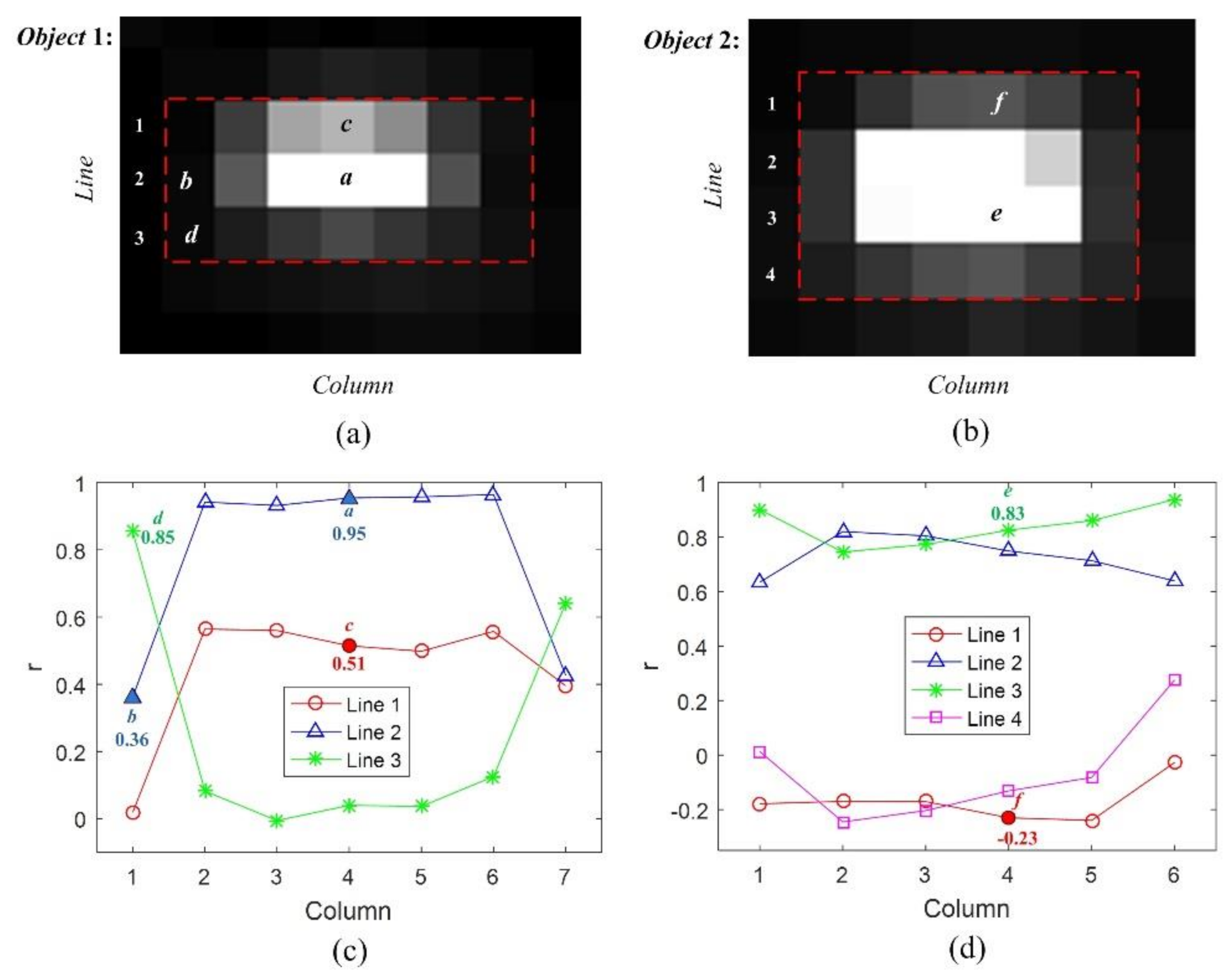
Correlation coefficients (denoted by r) are used to measure the degree of correlation between the data and models. Usually, the object streak center occupies one or two lines of pixels, and we call the two types of object streaks Ob 1 and Ob 2, as shown in Figure 2a,b. 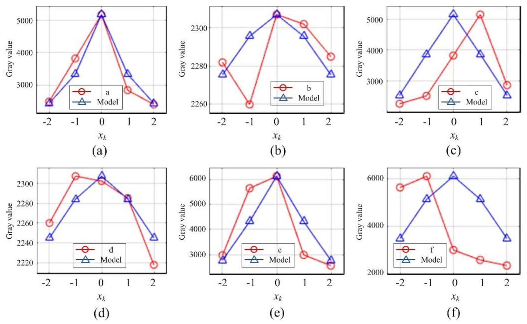We take the position of each pixel in the red dotted lines as the longitudinal center to conduct model fitting, and the correlation coefficients are shown in Figure 2c,d. Six pixels in different positions of the two objects, including object centers, object edges and image backgrounds, are focused on, and their data and Gaussian models are shown in Figure 3.

It can be seen that the correlation coefficients are more than 0.9 from the center of Ob 1 to the horizontal edges, which means that there is a high correlation. However, the correlation at the background 1 is weak and less than 0.5. Line1 and Line3 are the two vertical edges of Ob 1, and the Gaussian models are slightly mismatched with the data, whose correlation coefficients are usually less than 0.6 but more than that of the image background 1. However, there is a background noise at image background 2 where the correlation coefficient is also high. The centers of Ob 2 are Line2 and Line3, and most of the correlation coefficients are between 0.6 and 0.9. Line1 and Line4 belong to the two vertical edges, and the Gaussian models are heavily mismatched with the data, so there is no correlation between the two.

If selected correlation coefficient thresholdings are low, objects with weak Gaussian morphology can be recognized well, but lots of false alarms appear, just like pixel d. Contrarily, if the thresholdings are high, the dim objects with low model correlation cannot be recognized. Therefore, the correlation coefficient thresholding is set to 0.5. On the premise that the objects and stars can be recognized, a few false alarms of background noise are considered to remove.

3.2. Standard Deviation

We take Figure 4a as an example to analyze the method of removing false alarms with standard deviation. First, all the pixels in the image are sorted by increasing gray values, and we calculate standard deviations of the minimum 1–100% pixels, which we call grayscale sequence method (GS). Based on experience, we start the calculation of the change rate of standard deviation from the minimum 90% pixels and control the calculation interval to reduce the number of calculations. When GS method is applied to large data sets, star image partitioning becomes more important. We divide the star image into multiple subimages and calculate the data in the regions of interest. The standard deviations that we obtain are increasing, and we analyze their change rate to find the mutation value where the standard deviation is the boundary between the objects and image backgrounds. The change rate of standard deviation is stable when the selected pixels are image backgrounds, and only when a large number of object pixels are selected does it fluctuate significantly. Therefore, the standard deviation thresholding selected with GS method has a certain hysteresis, and a part of the dark objects and stars may be filtered out.

If the standard deviation corresponds to the object itself rather than the variation trend of image grayscales, the hysteresis can be avoided. We consider our column recognition method where five data are grouped, and the standard deviations of all the groups are calculated and sorted incrementally, which we call standard deviation sequence method (SDS). Since the standard deviation represents the fluctuant characteristics of the object or background, the change rate changes significantly when it is converting from the image backgrounds to the dark objects. The results of thresholding selection in both methods are shown in Figure 4. In Figure 4b,d, a mutation value is greater than all previous values, and there is a relatively large increase in the mean value of a certain interval of the same size before and after this value. However, we cannot expect how significant the mutation of the change rate at this value is, because it is in a short transition interval, after which the change rate increases rapidly. What we can do is to find an optimal value within the transition interval and to obtain the standard deviation at the position of the optimal value as thresholding for the segmentation of backgrounds and dark objects.

The results show that the selected thresholdings with both methods are respectively 11.4 and 7.29, and we will verify the effectiveness of SDS method in Section 4.2. If the standard deviation of a group of data is less than 7.29, we regard it as a background directly and there is no need to model, which reduces 71% time of model fitting and avoid the risk of misidentifying the background data with Gaussian morphology as the target data. Of course, if the standard deviation of a group of data is greater than 7.29, we cannot rule out the possibility that it is a bad pixel or background noise.

3.3. K Value

The mean square error values between the data and models differ greatly due to the different amplitudes of models, and mean square error values at the object are much larger than those at the background, which does not mean that the fitting effect at the background is better. Therefore, it is crucial to unify the mean square error values for the object models of different amplitudes.

The mean square error represents the degree of deviation between the model and the data, whereas the variance represents the degree of fluctuation of the data. Now, the ratio of the two is defined as

$$K=\frac{MSE}{D\left(y\right)}=\frac{{\displaystyle \sum {\left({\tilde{y}}_k-y_k\right)}^2}/n}{{\displaystyle \sum {\left(y_k-m\right)}^2}/n-1}$$

(10)

where MSE is mean square error, D(y) is the variance, m is the mean value of a group of data, n is the number of data points, and K means the mean square error between the model and the data under unit fluctuation.

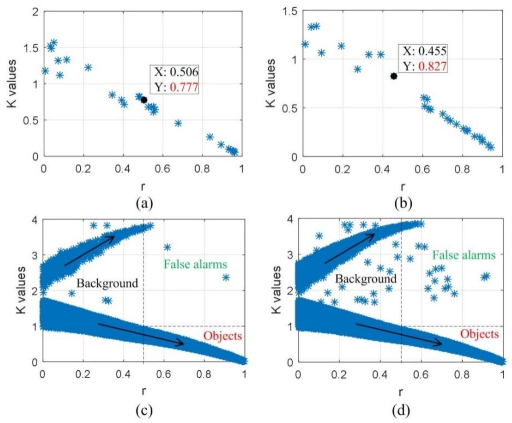
We analyze K values in Ob 1 and Ob 2. It is found that K values are small when the correlation coefficients are large, and there is an obvious linear relation. When r is 0.5, both K values are less than 1, as shown in Figure 5a,b. For a star image containing more objects, the relation between K values and correlation coefficients is shown in Figure 5c,d. Some K values decrease with the increase of r, and K values of another part increase with the increase of r. Others have no regular distribution, but they are all greater than the K value when r is 0.5. We think r ≈ 0 means that there is no correlation between the two groups of data, which are orthogonal. At this time, it can be approximately regarded as random noises with the equal mean.

Finally, we can filter out the false alarms by setting K thresholding. We focuses on the part where r is greater than 0.5 and K values decrease with the increase of r, and it reflects the significant Gaussian morphology of the image data and has a high correlation with the model. From Figure 5, K value is 1 when r is 0.5, and the false alarm pixels are randomly distributed in the places where K value is greater than 1.5. Therefore, we chose k = 1 (of course, any value between 1 and 1.5) for K thresholding. Other parts are background noises, bad pixels and the edges of objects. In this way, the objects and stars can be well segmented from the star image.

4. Experimental Results

In the experiment, real and simulated star images in different scenes are used to verify the effectiveness of our proposed correlation segmentation method. First, we analyzed the problems existing in the segmentation process through the experiments of two simple scenes, and demonstrated the effect of horizontal supplementary recognition. Second, we verified the validity of the SDS method. Then, the results of our proposed method are compared with traditional threshold segmentation methods in complex backgrounds. Finally, the identification rate and false alarm rate of our method in complex backgrounds are obtained based on two special scenes with 2000 frames each.

4.1. Horizontal Supplementary Recognition

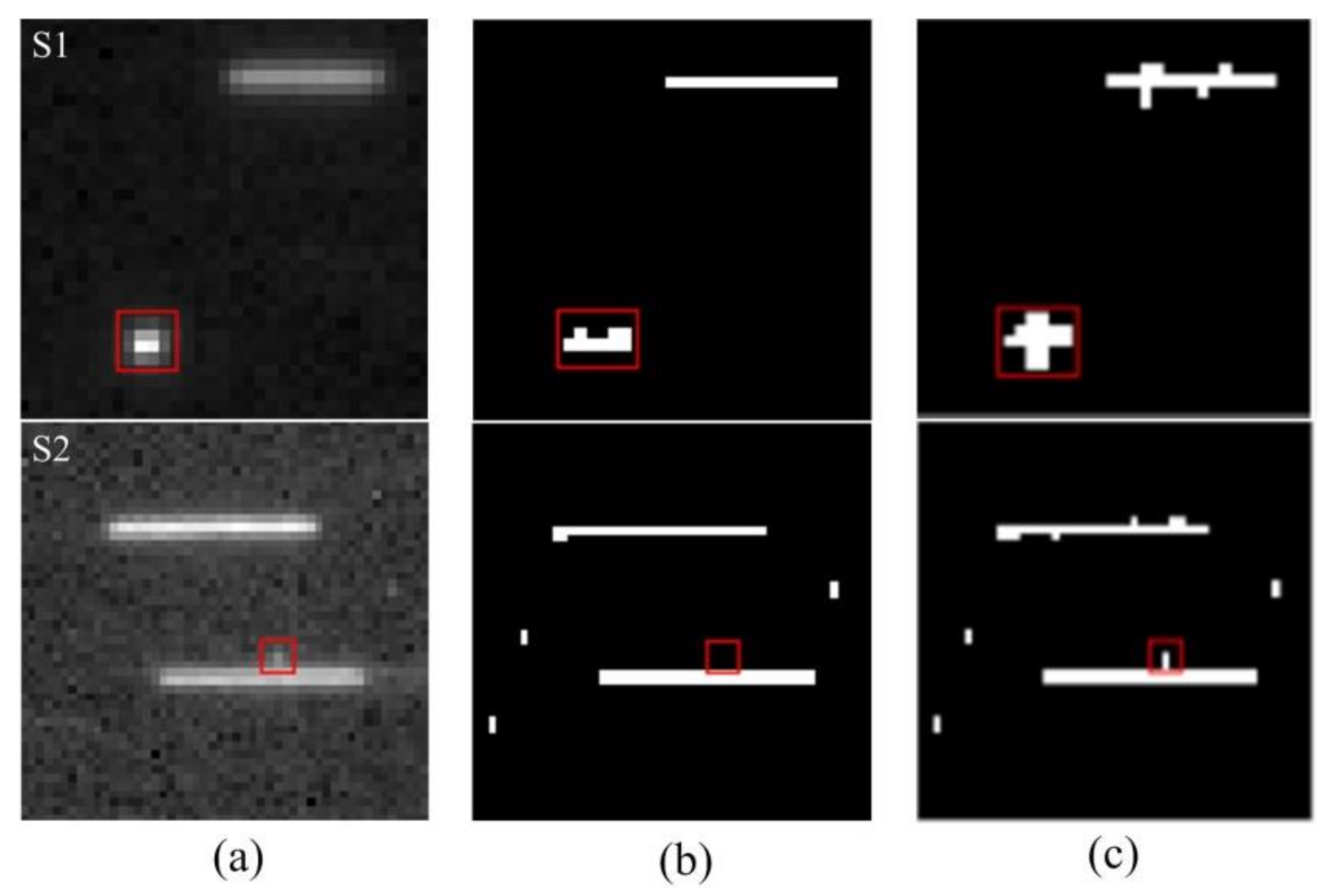
The correlation segmentation method can recognize and extract point targets and streaks with 1D Gaussian morphology. We choose two simple scenes for analysis, and the difference between the two scenes is whether a point object in the image is close to a streak, as shown in Figure 6. It is found that the vertical Gaussian features of objects at the upper and lower edges are not significant, so the identified point object is a strip and the longitudinal edges are lost. Besides, when an object and a star are approaching vertically, the column recognition method is influenced, making the point object unrecognizable. Therefore, the horizontal supplementary recognition should be carried out at the upper and lower lines (about 2 lines) of the identified objects and stars by using the same modeling method. This has a good supplementary effect on point object recognition but only has low impact on the recognition of extending object streaks.

4.2. Comparison of GS Method and SDS Method

For bright objects, the star image can be well segmented by using the correlation segmentation method combined with the standard deviation thresholding selected with the two methods in Section 3.2, and the difference is that the lower standard deviation thresholding slightly results in more noise points. However, for a dark object without clear contour and significant Gaussian morphology, the SDS method has obvious advantages, as shown in Figure 7.

We analyze the recognized pixel number of the five objects in different σ thresholdings. When the σ thresholding is more than 24.2, the pixel number begins to decrease, which means that part edges of the objects are filtered out, as shown in Figure 7d. The thresholding obtained with SDS method, 24.11, is perfectly consistent with the optimal thresholding, 24.2. This result proves that the SDS method is more valid, and it can identify the dark objects and can also filter out most of the noises. Although the removal effect of background noises with GS method is good, it makes the object recognition incomplete or impossible.

4.3. Comparison of Segmentation Methods

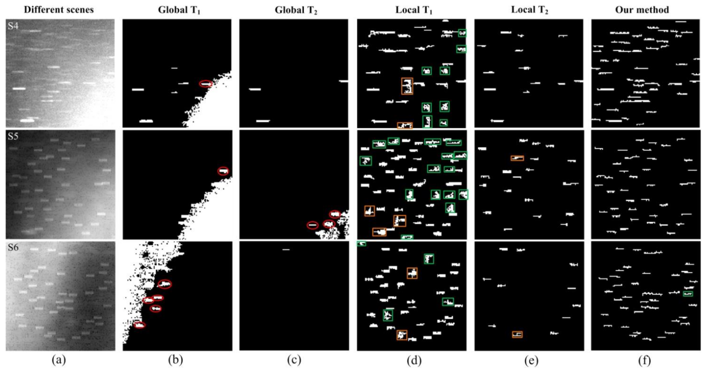
In order to verify the effectiveness of our proposed star image segmentation method combining correlation coefficient, standard deviation and K value, the global and local thresholding segmentation methods are used for comparison. We use the statistical method to set the thresholdings: T₁ = μ + σ and T₂ = μ + 2σ. The local thresholding method has different segmentation results due to different sub-blocks, so the principle of the sub-block size is that the minimum false alarms are produced on the basis of identifying more objects. In the comparison, an object streak whose recognition length is more than half of its length is considered to identify successfully, otherwise, the objects are not reflected in the figures. If multiple objects that overlap in original images are identified as an extended object streak whose shape is easy to distinguish, we count according to the original image. The results are shown in Figure 8.

The star images with a size of 120 × 120 pixels have uneven backgrounds. The recognition results are terrible under low and high global thresholdings, and the results of local thresholding segmentation are obviously better. However, the contours of some objects are not clear, and there are many false alarms caused by the selection of windows. We find that gray thresholding segmentation has poor adaptability, and our proposed segmentation method is more effective and identifies more objects. The segmentation results of different star images with different methods are shown in

Table 1. Segmentation results of different star images with different methods.

	Scenes	Global Methods		Local Methods		Our Method
		T1	T2	T1	T2
Number of recognized objects	S4	6	3	27	13	47
	S5	1	3	34	21	40
	S6	5	1	30	11	40
Number of false alarms	S4	Heavy	0	8	0	0
	S5	Heavy	Slight	15	0	0
	S6	Heavy	0	4	0	1

.

In addition, we respectively simulated 2000 frames based on the backgrounds of S5 and S6. Forty target streaks in each frame were randomly distributed, and the recognition rate and false alarm rate were calculated. The recognition results are shown in

Table 2. Recognition results of simulation star images with 2000 frames each (m: mean, σ: standard deviation).

Scenes	The Number of Recognized Objects		Recognition Rate	The Number of False Alarms		False Alarm Rate	Algorithm Speed (s)
	m	σ		m	σ
S5	39.02	1.08	97.6%	0.17	0.47	0.43%	0.29
S6	39.16	1.05	97.9%	0.19	0.51	0.48%	0.30

. Our correlation segmentation method ensures low false alarm rate and achieves high recognition rate. Of course, both metrics are influenced by many factors, such as the noise level, target intensity, background complexity, and threshold selection. For star image recognition, in order to achieve better recognition rate, we can reduce each thresholding at the cost of increasing false alarm rate. Therefore, a balance between the two needs to be struck according to application environments. Moreover, the large fluctuation of image backgrounds and the low target intensity has a great impact on target recognition.

For the star images with a size of 120 × 120 pixels, we run our algorithm on the platform of Intel Core i5-6500 CPU 3.2GHz, MATLAB2016a, and the average calculation time of our method is about 0.3s. For ground-based telescope observation, the exposure time is generally at second level. When processing star images with complex backgrounds, we often select some areas of interest with small sizes. Therefore, it meets the real-time requirements. Through the simulation experiments of 2000 frames each, the recognition rate of more than 97% and false alarm rate of less than 0.5% can be stably obtained by our method.

The grayscale values of image backgrounds change greatly everywhere, so it is obviously impossible to select a certain global thresholding to separate all the objects from the backgrounds. However, the local thresholding method needs to select appropriate sub-blocks according to the size of the objects. In addition, it should not only ensure that the complete object is in the same sub-block but also ensure that there must be objects in each sub-block, otherwise there are many problems such as false alarms and incomplete object recognition across sub-blocks. For a star image with a large number of objects, it is difficult to satisfy the two situations. Our proposed correlation segmentation method solves the problems well and overcomes the limitation of gray segmentation.

5. Conclusions

The influence of clouds and moonlight is a challenge for star image segmentation, and local thresholding methods can slightly improve but not well overcome it. We present a new star image segmentation method, and the correlation coefficients between the data and models are used to segment star images. In addition, the standard deviation thresholding and K value are combined to remove false alarms. The results show that our proposed method works well in complex background, which can be used for object detecting and tracking in the cloudy and bright moonlit night and can be applied in machine learning system for astronomical observation and object classification.