Article

HSB-SPAM: An Efficient Image Filtering Detection Technique

1
Amity School of Engineering & Technology, Amity University Uttar Pradesh, Noida 201301, India
2
Department of Cyber Security, Kyungil University, Gyeongbuk 38428, Korea
*
Author to whom correspondence should be addressed.
Appl. Sci. 2021, 11(9), 3749; https://doi.org/10.3390/app11093749
Submission received: 23 March 2021 / Revised: 14 April 2021 / Accepted: 16 April 2021 / Published: 21 April 2021
(This article belongs to the Special Issue Development of IoE Applications for Multimedia Security)

Abstract

:
Median filtering is being used extensively for image enhancement and anti-forensics. It is also being used to disguise the traces of image processing operations such as JPEG compression and image resampling when utilized in image de-noising and smoothing tool. In this paper, a robust image forensic technique namely HSB-SPAM is proposed to assist in median filtering detection. The proposed technique considers the higher significant bit-plane (HSB) of the image to highlight the statistical changes efficiently. Further, multiple difference arrays along with the first order pixel difference is used to separate the pixel difference, and Laplacian pixel difference is applied to extract a robust feature set. To compact the size of feature vectors, the operation of thresholding on the difference arrays is also utilized. As a result, the proposed detector is able to detect median, mean and Gaussian filtering operations with higher accuracy than the existing detectors. In the experimental results, the performance of the proposed detector is validated on the small size and post JPEG compressed images, where it is shown that the proposed method outperforms the state of art detectors in the most of the cases.

1. Introduction

Today, most of the communication is being done in digital form, which opens a Pandora box of security attacks such as editing, copying, deleting and so on. Sometimes, the editing operation which does not require any expertise due to the wide availability of ubiquitous digital imaging devices and sophisticated editing software, may create an uproar as fake (edited) images and can be circulated through popular social media platforms to mislead the users as shown in Figure 1. Figure 1a shows that the anti-gun activist and student Emma Gonzalez is tearing the copy of US constitution.
Whereas, the real picture is shown on the right side published in Teen Vogue magazine that is tearing the gun range target photo. The fake image was circulated on social media more than 70,000 times to get some political mileage in 2018. Therefore, the need of forensic toolboxes is required strongly which can assess blindly the authenticity of digital images without access to the source image, source device or the aid of an auxiliary watermark signal.
In the recent years, image forgery detection techniques [1,2,3] based on handcrafted features and CNN features have been introduced. Matern et al. [1] proposed a physics-based method that considers the 2-D lighting environments of objects. The incident of the light assists in detecting fake objects in the image. The method is verified on high-resolution challenging databases and has proved its superiority for some existing techniques, however there is still sufficient gap for improvement. Moghaddasi et al. [2] exploited the discrete cosine transform (DCT) domain and singular value decomposition for image forgery detection. The method uses moments as features and support vector machine (SVM) as a classifier. The authors claim the good accuracy on multiple databases although performance may be degraded on cross-dataset and unknown image. Deep networks are found effective in many applications like face reorganization [4], object classification [5], facial expression [6] and so on. Marra et al. [3] proposed a CNN based feature extractor for high-resolution images. Unlike other CNN techniques, the gradient check-pointing is applied for feature extraction on entire original image size. Marra et al.’s technique extracts better features than other techniques in which the image is divided into overlapping patches to extract features. However, it has a high computational cost as full-size images are being used in feature extraction. In addition to the aforementioned handcrafted features and CNN features-based techniques, there has been discussed several image forgery detection techniques which are based on hardware or camera fingerprints, lighting environment, illumination, statistical information, deep networks and so on. In spite of this, some techniques [7,8,9] are also designed to counter image forensic and forgery detection techniques. Marra et al. [7] designed the technique to counter the image forgery detection techniques. Kim et al. [8] applied the adversarial Networks to remove the artifacts of median filtering. Gragnaniello et al. [9] discovered that CNN based techniques are easy to conquer than machine learning based image forgery detection techniques while fake images are generated by an adversarial network.
To make the fake images more realistic, the malicious intent people use multiple operations such as rotation, resampling, contrast enhancement so that the traces of modifications are hidden. Thus, the performance of image forgery detection methods is adversely affected by the filtering operations such as median filter, Gaussian filter, and mean filter. In particular, the median filtering (MF) is preferred among some forgers because it has the characteristics of nonlinear filtering based on order statistics. Therefore, a Markov chain based median filtering detector using a high significant bit-plane is proposed in this paper. The Markov chain is popular in many applications such as steganalysis, object classification, atmospheric science, and even in median filtering detection. The prominent median filter detector using Markov Chain was proposed by Kirchner and Fridrich [10] which uses difference arrays for Markov chain. Alike method is also proposed by Pevny et al. [11] for steganalysis and popularly known as SPAM. The method extracts features using Markov chain on thresholded difference array that results into more granular collection of features and ultimately leads to a higher accuracy. Chen et al. [12] considered the absolute difference while applying thresholding to minimize the size of feature set so that the complexity of the method can be reduced. Cao et al. [13] calculate the variance of difference arrays and use the probability of zero elements to decide whether an image is median filtered or not. Cao et al.’s method is close to Markov model. Agarwal and Chand [14] extended the work of Kirchner and Fridrich’s method [10] by considering higher order differences. The incorporation of higher order differences collects even the minute details of images that help in effective collection of feature sets. The extraction of features is executed with the help of Markov chain on the first, second and third order thresholded difference arrays. Thus, Agarwal and Chand’s method could improve upon Kirchner and Fridrich’s method. However, it has been observed that the thresholded array and absolute difference can be loose some relevant information which may be useful in more accurate detection. In this paper, a high significant bit-plane based image forgery detection strategy is proposed to retain vital information. The main contributions of the proposed method can be summarized as follows:
  • The proposed scheme can reduce the bit depth to attain more relevant information in difference arrays. Higher significant bit-planes are considered for strong statistical analysis.
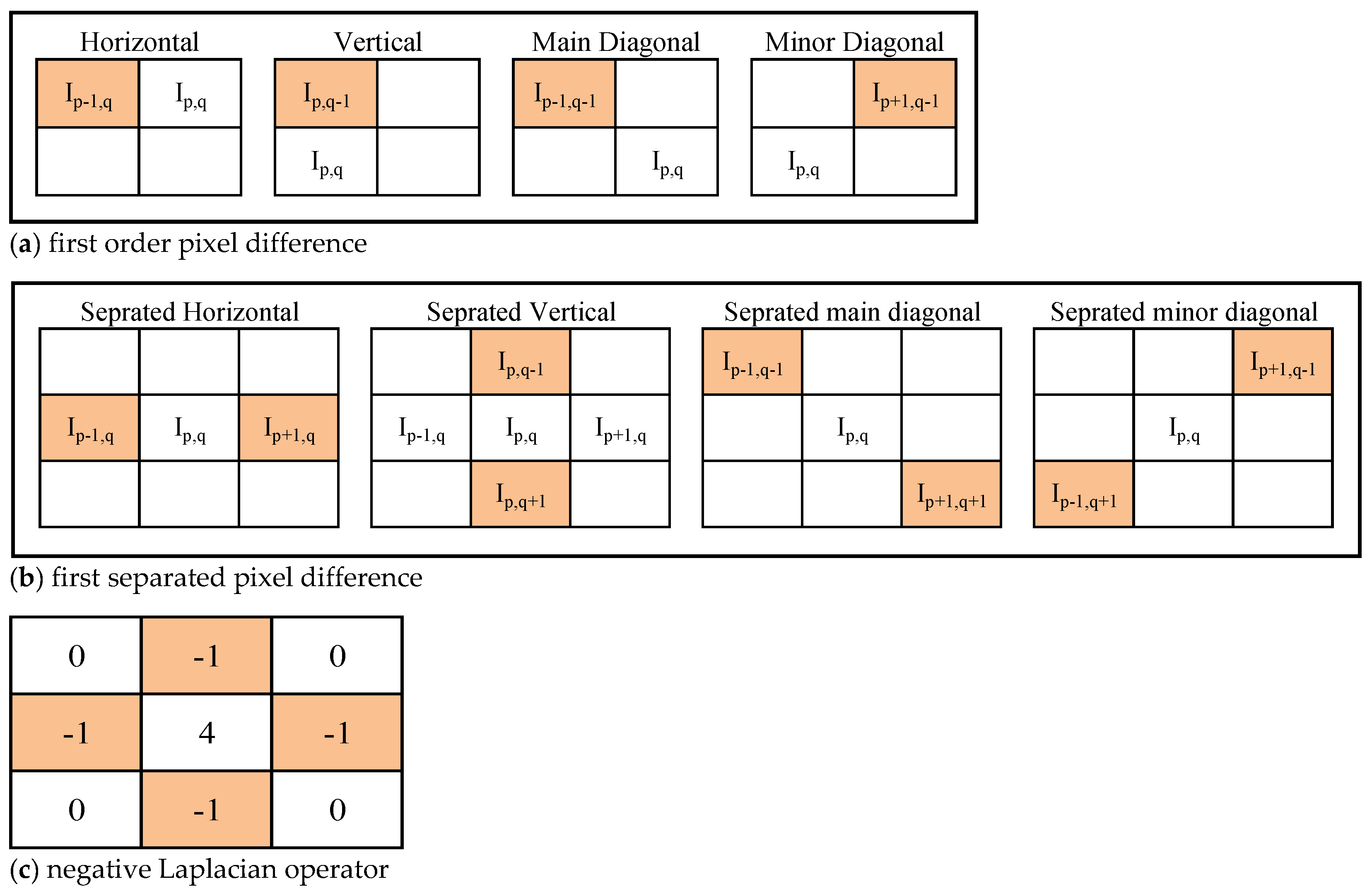
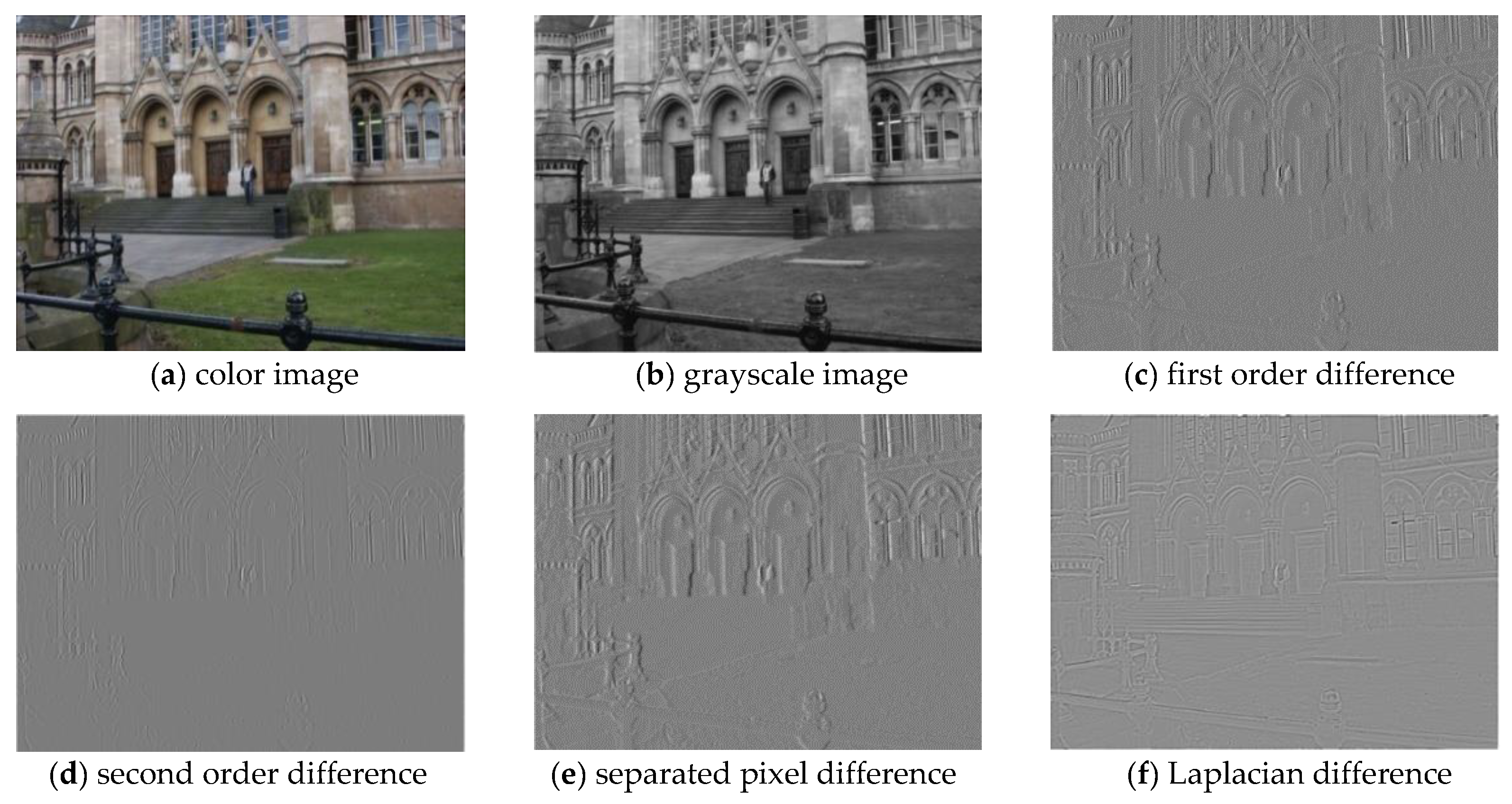
  • Various derivatives such as pixel difference, separate pixel difference, and the Laplacian operator are considered for a robust feature vector that can help in collecting additional information so that accuracy can be further enhanced. Further, the co-occurrence statistics is extracted from derivatives using the Markov chain.
  • Experimental results are compared with some of the popular methods such as GLF, GDCTF, PERB and SPAM to evaluate the performance of the proposed scheme. For the exhaustive analysis, the experimental results are shown for median filtered, mean filtered and Gaussian filtered images.
  • The experimental analysis shows that the proposed method has better performance than existing methods in most of the scenarios. There is a significant improvement of more than 2% in detection accuracy for the case of 3 × 3 size filter on the low-resolution images and highly compressed images.
The rest of the paper is organized as follows. In Section 2, existing techniques are discussed. The proposed technique is elaborated in Section 3. In Section 4 and Section 5, experiment results and conclusion of the paper are discussed respectively.

2. Related Work

In this section, the existing and popular filtering detection techniques are briefly reviewed. It has been observed that there are many works [10,12,13,14,15,16,17,18,19,20,21,22,23,24,25,26,27,28,29,30,31,32,33,34,35] for detecting filtering in which most of works give emphasis on median filtering detection due to its non-linear nature. Only some methods in [10,23] exist for detecting Gaussian filtering and for median, mean and Gaussian filtering in [23,24,31]. The existing techniques can be categorized as the autoregressive model, the CNN model, frequency domain, and Markov chain.
Kang et al. [16] introduced the autoregressive model for median filtering detection. Median filter residuals are considered and three median filter residuals arrays are generated after applying median filter of different size. The size of feature vector is small though a performance degrades on low resolution images. Ferreira and Rocha [17] also generated numerous median filter residuals arrays after applying median filter multiple times. The eight quality matrices are calculated on residual arrays. The SVM classifier is applied to classify the images using quality matrices as a feature vector. The method fails on low resolution and compressed images. Yang et al. [21] proposed a two dimensional autoregressive (2D-AR) model. The 2D-AR model was applied on median filtered residual (MFR), average filtered residual (AFR) and Gaussian filtered residual (GFR). Multiple residuals are still considered the accuracy decreases on small sized images. Rhee [27] proposed a technique that utilizes the autoregressive model, edge detectors and Hu moments. The hybrid feature set is not able to tackle the compression issue. In addition, Rhee [28] also applied the autoregressive model on bit plane sliced images. Rhee applied the autoregressive model on bit plane sliced median filtered residual arrays. The least and highest significant bits are considered and the performance is verified on resampled images. Peng et al. [31] proposed a hybrid feature set using autoregressive model and local binary pattern (LBP) operator. The proposed model was able to classify median, mean and Gaussian filtered images. Chen et al. [18] introduced the convolutional neural network (CNN) for median filtering detection. The new CNN layer is introduced to provide median filter residual. The performance of method is superseded by Tang et al. [22] by proposing a CNN model using two multilayer perceptron (mlpconv) layers. The mlpconv layer is claimed more suitable for nonlinear data learning. Bayar and Stamm [23] introduced a constrained convolutional layer to highlight the image features. The method can detect median filtering, Gaussian blurring, resampling and JPEG compression. Luo et al. [29] applied the high pass filter on the image and resultant image is given as input to CNN. Zhang et al. [35] proposed a CNN model by introducing an adaptive filtering layer (AFL). The proposed AFL is constructed to capture the frequency traces of median filtering in the DCT domain. The performance of CNN techniques is satisfactory on low resolution images although computation cost is very high and is required large dataset for training.
Hwang and Rhee [19] proposed a method for Gaussian filtering detection. The Gaussian filter residual and frequency transform residual features are utilized for detection. The fast Fourier transform is used to convert from the spatial domain to the frequency domain. Liu et al. [20] also considered the Fourier transform for the frequency domain. In Liu’s method, it is discovered that most of the values are zero in a low-frequency region of the median filtered image in contrast to a non-filtered image. Wang and Gao [24] proposed a local quadruple pattern and extracted features in discrete cosine transform (DCT) to detect median, mean and Gaussian filtering. Li et al. [25] also proposed a method using the DCT domain. The addition of absolute differences of DCT coefficients are calculated on sequential median filtered images. The SVM classifier is used to classify the images. Gupta and Singhal [30] proposed a 4-dimension feature set using median filter residual in DCT domain. Hwang and Rhee [32] discussed a 10-dimension feature set for Gaussian filtering detection. The amount of blurring is calculated from Gaussian filtered images of ten different filter size. The frequency-based techniques are not giving the good results as the change in domain loose important statistical information. Kirchner and Fridrich [10] considered the difference arrays for median filtering detection. The ratio of difference arrays histogram bins is analyzed to discover uncompressed median filtered images. The authors also proposed a technique for a compressed median filtered images using Markov chain on difference arrays although detection accuracy is low on the small size images. Chen et al. [12] proposed a hybrid feature set using global and local features. Global features are extracted using the Markov chain and local features using normalized cross correlation on difference arrays. The absolute difference is considered while applying the Markov chain on difference arrays. The absolute difference loses the vital information change. Agarwal and Chand [14] applied the Markov chain on the first, second and third order difference arrays. There is performance gain by considering a higher order differences. Niu et al. [15] combined the features of uniform local binary pattern and Markov model for better results. Peng et al. [26] considers multiple residuals-first order difference, median filtering residual, and median filtering residual difference. The autoregressive model and the Markov chain are applied to fetch statistical information from multiple residuals. Gao and Gao [33] applied the autoregressive model in the frequency domain and the Markov chain in the spatial domain. The method applied on difference arrays in multiple directions. Gao et al. [34] combined two feature sets—Markov chain and local configuration patterns features, where the combined feature set approach gives slight performance improvement. In the most of the Markov chain based methods [10,12,13,15,26,33,34], the SVM classifier is utilized to classify into non-filtered and median filtered images, where the linear discriminant analysis classifier is applied for classification. Markov chain represents the co-occurrence of elements in a better way in comparison with the autoregressive model and the frequency domain based methods. There is sufficient loss of statistical information while converting from spatial to frequency domain. The autoregressive model gives a small size feature vector but there is a need of optimizable parameters for training of each scenario (JPEG compression, image size). Further, experimental analysis showed that the performance of many methods based on autoregressive and frequency domain is good only due to zero padding artifacts. The computation cost of CNN based methods is very high and also there is a need of large dataset for training. In this paper, Markov chain is utilized in spatial domain for its simplicity and robustness. The proposed work is discussed in the next section.

3. The Proposed Method

The proposed method consists of two phases namely feature extraction, and training and classification. The contribution of the proposed method lies in the feature extraction phase in major. For an elaborative study and analysis, the feature extraction phase is subdivided into a higher significant bit-plane analysis and pixel difference arrays and Markov chain sub-phases. In this section, a higher significant bit-plane analysis is described followed by a discussion on pixel difference arrays and the Markov chain.

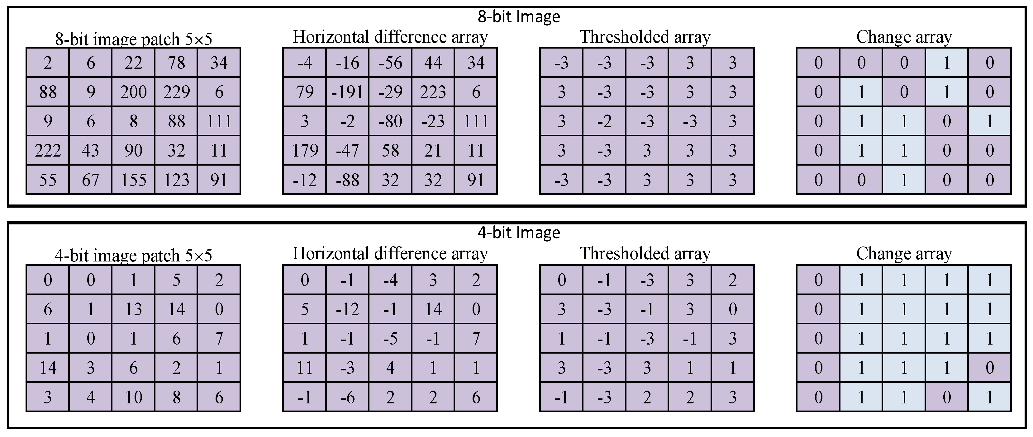
3.1. Higher Significant Bit-Plane Analysis

In order to collect more valuable statistical information, the proposed method transforms the image into a higher significant bit-plane based image by dropping least significant bits of each pixels and considering only the higher significant bits. The resultant image contains more relevant information in particular range that helps in generating more valuable information with difference arrays than the complete image. To study experimentally and analyze the effectiveness of the higher significant bit-plane based image, a normal probability distribution of pixel difference in the UCID database [36] having 1338 images is considered. The graph of the normal probability distribution is shown in Figure 2, where ORI denotes the non-filtered image, ORI_HSB denotes the higher significant bit-plane based image of ORI images. In general, the 8-bit grayscale image is considered by conventional image filtering detection techniques. However, 4-HSB version of images is considered in this paper. Median filtered image with filter size 3 × 3 and 5 × 5 are denoted as MF3 and MF5 and their corresponding higher significant bit-plane versions are denoted by MF3_HSB and MF5_HSB. In the same way, mean and Gaussian filtered images with filter size 3 × 3 & 5 × 5 are denoted as AVG3, AVG5, GAU3 & GAU5, respectively. It is evident from the Figure 2 that the higher significant bit-plane filtered images (MF3_HSB, MF5_HSB, AVG3_HSB, AVG5_HSB, GAU3_HSB, GAU5_HSB) contain a most of the information in small interval whereas the information is distributed into a large interval in normal images. Since the Markov chain is applied on thresholded arrays, the higher significant bit-plane images will perform better in the view of thresholding.
To further verify the benefit of higher significant bit-plane images, entropy of the first order pixel difference arrays is calculated from the non-filtered and filtered images. The entropy dissimilarity of pair ORI and MF3 is less in comparison with pair ORI_HSB and MF3_HSB. The high dissimilarity of low-bit filtered and low-bit non-filtered images give better detection capability. The main reason is that difference array of higher significant bit-plane images performs better. Further, the dissimilarity pattern is also followed by MF5, AVG3, AVG5, GAU3 and GAU5 filtered images as shown in Figure 3.
As discussed above, the Markov chain is applied on thresholded difference arrays to extract statistical information in compact array, the higher significant bit-plane images provides better information for feature sets without increasing the size of feature vector. The validation of performance benefits in the higher significant bit-plane images is illustrated in Figure 4. In the example, a 5 × 5 size pixels image patched from 8-bit image is considered as 8-bit image is commonly used for experimental analysis. The horizontal difference array of the image is further thresholded at threshold Γ = 3. To analyze the variation in information, the change array is constructed. The change array shows the change in the element value of column wise. Since the initial three values are −3 in the first row of thresholded array, there is no change and it is represented in the change array as 0. The fourth value in the first row of thresholded array is three. It means that the value is changed from −3 to 3. Therefore, the change is represented by one. The same analysis is performed on 4-HSB image of the same 8-bit image which is considered in the aforementioned case. It can be seen in the thresholded array and change array that shows better variation on 4-HSB image means that the statistical analysis performed on HSB image will demonstrate better filtering detection accuracy.
In addition to 4-HSB depth, other bit-depths can be also considered as a base on the image data set characteristics. However, it has been observed from the experimental analysis that selection of 4-HSB depth has been the most appropriate for high accuracy. In the next sub-section, the discussion regarding multiple pixel difference arrays is provided to extract robust statistical information, which is followed by the discussion of Markov chain to extract feature vector on the difference arrays.

3.2. Pixel Difference Arrays and Markov Chain

The first order pixel difference array and Markov chain has been used in literature to extract the feature set. The extracted set of features has been used to train the classifier that would be used for classification of images finally. The first order pixel difference array contains from range −255 to 255 in the case of 8-bit image. The first order pixel difference array in the vertical direction can be represented as follows for an image I :
∇↓p,q = Ip,qIp,q+1
Similarly, first order pixel difference arrays in horizontal, main diagonal, and minor diagonal directions can be calculated as per the Figure 5a.
Based on the aforementioned discussion in the Section 2, it is found that the incorporation of second and higher order pixel difference arrays has resulted in better accuracy as additional information is extracted by the incorporation of second and higher order pixel difference arrays. However, there are some shortcomings of higher order pixel difference arrays that are discussed in forthcoming contents.
The second order pixel difference array contains from range −510 to 510 in the case of 8-bit image. The thresholding loose more information in the second order pixel difference array in comparison to the first order pixel difference array because the range of elements is higher than the first order. Therefore, separated pixel difference array, which provides additional information, and with intact range of elements, −255 to 255, are being used instead of the second order pixel difference array. For an image I , the separated pixel difference array in vertical direction can be represented as follows:
∇↓sp,q = Ip,qIp+2,q
Likewise, the separated pixel difference arrays in horizontal, main diagonal, and minor diagonal directions can be calculated as shown in the Figure 5b.
In addition to the first order and separated pixel difference arrays, Laplacian operator can also provide more suitable statistical information as it highlights abrupt changes clearly and provides the combined statistical information of horizontal and vertical neighbors. So, the proposed detector makes use of negative Laplacian operator to get the Laplacian difference array. The Laplacian operator can be defined as shown in Figure 5c:
Lp,q = 4 × Ip,q − (Ip+1,q + Ip−1,q + Ip,q+1 + Ip,q−1)
The image and its corresponding difference arrays—the first order, the second order in the vertical direction, the separated pixel and Laplacian—are all shown in Figure 6. It is evident that each difference array provides the constructive statistical information of the image. Therefore, the features are extracted from the first order pixel difference arrays, separated pixel difference arrays in vertical, horizontal, diagonal, minor diagonal directions and Laplacian difference arrays in the low bit image, which helps in achieving better performance.
Next, the second order Markov chain is extracted to identify the co-occurrences of difference pixel arrays. Before understanding the second order Markov chain, we have to understand the first order Markov chain firstly. The first order Markov chain for the thresholded vertical first order pixel difference array ( ) can be defined as follows:
χα,β = Pr(∇↓p,q+1 = α | ∇↓p,q = β)
where χ α , β = 0 for P r ( p , q = β ) = 0 . The second order Markov model can be defined for the thresholded vertical first order pixel difference array ( ) :
χα,β,γ = Pr(∇↓p,q+2 = α | ∇↓p,q+1 = β, ∇↓p,q = γ)
where α , β , γ { Γ , Γ + 1 , 0 , , Γ 1 , Γ } and χ α , β , γ = 0 for P r ( p , q + 1 = β , p , q = γ ) = 0 in addition.
Thus, nine feature vectors ( Ω 1 , Ω 2 , Ω 3 , Ω 4 , Ω 5 , Ω 6 , Ω 7 , Ω 8 , Ω 9 ) are fetched using the Markov chain corresponding to the first order and separated pixel difference arrays in vertical, horizontal, diagonal and minor diagonal directions and the Laplacian difference array. The average of vertical and horizontal difference arrays feature vectors is considered. Similarly, the average value is taken for diagonal and minor diagonal feature vectors. The average is considered to normalize the varying characteristics to the flipping and mirroring operations. Finally, the final feature vector can be defined as follows:
Ω = ( Ω 1 + Ω 2 ) 2 + ( Ω 3 + Ω 4 ) 2 + ( Ω 5 + Ω 6 ) 2 + ( Ω 7 + Ω 8 ) 2 + Ω 9
The dimension of resultant feature array can be obtained by following equation:
| Ω | = ( | Ω 1 | + | Ω 2 | ) 2 + ( | Ω 3 | + | Ω 4 | ) 2 + ( | Ω 5 | + | Ω 6 | ) 2 + ( | Ω 7 | + | Ω 8 | ) 2 + | Ω 9 |
|Ω| = 3 × (2 × Γ + 1)3
The second order Markov chain generates ( 2 × Γ + 1 ) 3 dimension array for the threshold ( Γ ). The detailed experimental analysis is performed to detect median, mean and Gaussian filtering on UCID database in the subsequent section.

4. Experimental Results

This section demonstrates the efficacy of the proposed method by carrying out an experimental study. The UCIDv2.0 [36] database (UCID) has been selected to evaluate the performance of the proposed method since the UCID database has been one of the prime databases being used in literature. All experimental results are shown using UCID database in Table 1, Table 2, Table 3, Table 4, Table 5 and Table 6 excepting Table 4, where multiple databases are used for experimental analysis. UCID contains 1338 images of size 384 × 512 and 512 × 384 pixels. However, the images of size 256 × 256, 128 × 128, 64 × 64, and 32 × 32 pixels are considered for experimental purposes by cropping center part of original images of UCID database images as shown in Figure 7b, which can eliminate the padding artifacts. In particular, zero padding artifacts are more of a serious concern in filtering detection. The performance of the proposed method (HSB-SPAM) is compared with some of the popular and closely related image forensic methods such as GLF [12], GDCTF [30], PERB [17], and SPAM [10].
The performance is evaluated by an average percentage accuracy on 100 training-testing pairs using two classifiers, namely support vector machines (SVM) and linear discriminant analysis (LDA). The analysis of experimental results is presented in four-subsections defined as follows.
Both uncompressed and compressed images with JPEG quality Q = {70,50,30} and size of 128 × 128, 64 × 64, and 32 × 32 pixels are used for experimental purposes. The non-filtered images are denoted by ORI. Median filtered images with a filter size of 3 × 3 are denoted by MF3. Similarly, mean filtered and Gaussian filtered images of a filter size 3 × 3 are denoted by AVG3 and GAU3, respectively. Median, mean and Gaussian filtered images of filter window size 5 × 5 are denoted by MF5, AVG5 and GAU5, respectively. The compression is applied after filtering, i.e., post JPEG compression in filtered images. The SVM classifier with linear kernel is taken as a classifier. More than one hundred training testing pairs are formed for unbiased result analysis. Both the training and testing set have an equal number of images. The experimental results are represented in the form of average detection accuracy and average percentage error. For the proposed method, optimum SVM hyper-parameters are achieved using minimum classification error plot as shown in Figure 8. The estimated and observed minimum classification error point denotes the estimated and observed error while considering different hyper parameter values in the process of Bayesian optimization. The best hyper-parameter point denotes the iteration of corresponding optimized hyper-parameters. The minimum error hyper-parameters point defines the iteration of respective hyper parameters that produce the observed minimum classification error. The ORI and MF3 images of image sizes 64 × 64 and JPEG Q = 50 are taken for parameter selection. The hyper-parameters are utilized for all other experimental results in rest of the paper.
Experimental results are discussed in two sections. In Section 4.1, results are discussed between non-filtered and filtered images in Table 1, Table 2 and Table 3 on UCID dataset and in Table 4 for large dataset. In Section 4.2, Table 5 displayed the results where both sets contain only filtered images either of different filter size, different filter or both. In Table 6, different sized filtered images are considered in the training and testing set.

4.1. Results for Non-Filtered and Filtered Images

In this section, results are displayed for non-filter vs. filtered images on different image size and compression quality. In Table 1, the percentage of detection error for ORI vs. MF3 and ORI vs. MF5 images is provided. The results of the proposed method (HSB-SPAM) are outstanding in the most of the cases as there is significant improvement on low resolution and compressed images. Best results of each case are highlighted by the shaded background in the tables. The detection of the 3 × 3 filter size median filtered images is challenging than the 5 × 5 filter size median filtered images. The performance of PERB and GDCTF methods are comparatively low. It shows that many existing techniques performance is good in the case of zero padded median filtered images only. Especially, the zero padding increases the occurrence of zero’s in the filtered image in small size images (Figure 7a). The higher number of zero’s helps the classifier to classify the images easily. To overcome the zero artifacts, the first filtering is applied on the large size image and then the required image size is cropped from the center region.
Table 1. Percentage of detection error onMF3 and MF5 images.
IMAGE SIZEJPEG
COM.
ORI vs. MF3ORI vs. MF5
GLFGDCTFPERBSPAMHSB-SPAMGLFGDCTFPERBSPAMHSB-SPAM
128 × 128No0.3812.676.320.000.380.768.045.280.000.83
Q = 706.5616.089.107.083.402.749.926.533.022.33
Q = 509.5117.2610.0011.914.793.5110.306.914.903.65
Q = 3012.0819.4111.4615.807.194.7910.817.607.534.38
64 × 64No0.5917.499.410.170.831.3510.247.990.171.39
Q = 709.4120.9014.4812.056.424.9311.8710.076.674.59
Q = 5013.3021.9714.7917.198.686.3913.2910.6310.245.94
Q = 3015.8323.4716.2221.8411.497.8314.7211.0412.156.98
32 × 32No1.0123.6813.680.281.351.7718.5311.010.422.12
Q = 7014.9325.6619.9719.5110.737.9220.1313.7511.468.40
Q = 5018.5427.9122.2623.9615.7310.1221.2114.5813.099.86
Q = 3021.9829.0923.6528.5819.4111.9122.1115.4517.6711.67
In Table 2, experimental results are shown for detection of non-filtered and mean filtered images, ORI vs. AVG3 and ORI vs. AVG5. The results are given for image size 128 × 128, 64 × 64 and 32 × 32. The different image set are constructed using post JPEG compression of quality Q = {70,50,30}. The detection of mean filtered images of 3 × 3 filter size is more challenging than the 5 × 5 filter size. The performance of the proposed method is better than GLF technique. The performance of GDCTF, PERB and SPAM is inferior in the most of the cases. Actually, the detection of median filtered is more challenging than any other filter because median filter is a non-linear filter.
Table 2. Percentage of detection error on AVG3 and AVG5 images.
IMAGE SIZEJPEG
COM.
ORI vs. AVG3ORI vs. AVG5
GLFGDCTFPERBSPAMHSB-SPAMGLFGDCTFPERBSPAMHSB-SPAM
128 × 128No0.635.115.630.450.560.562.363.400.660.76
Q = 701.464.356.112.920.901.153.993.851.390.76
Q = 501.465.216.084.761.011.604.653.922.401.15
Q = 301.816.226.886.390.971.674.973.652.601.56
64 × 64No1.398.538.751.911.491.326.015.731.530.69
Q = 703.729.1910.075.733.332.927.337.573.921.91
Q = 504.9310.3110.497.994.413.198.027.675.492.19
Q = 306.3912.6311.1110.145.733.338.657.405.422.78
32 × 32No1.5315.6912.262.712.262.1914.249.032.641.25
Q = 706.1518.5314.629.795.184.7615.7311.227.124.10
Q = 508.8519.3615.6613.267.795.9016.6011.288.514.79
Q = 3011.1820.0315.9715.699.836.1818.0610.739.835.59
The Gaussian filter is also used to hide the traces of forgery. From analysis of experimental results provided in Table 3, the detection of Gaussian filtered images is more challenging than the mean filtered images though less challenging than median filtered images. Even for small size, 32 × 32 pixels and JPEG Q = 30, the proposed method gives more than 88% and 91% detection accuracy for GAU3 and GAU5, respectively. PERB method [8] give slightly better results for large size (128 × 128) and uncompressed image set for the Gaussian filter 3 × 3. However, the computation cost of PERB is the highest.
Table 3. Percentage of detection error onGAU3 and GAU5 images.
IMAGE SIZEJPEG
COM.
ORI vs. GAU3ORI vs. GAU5
GLFGDCTFPERBSPAMHSB-SPAMGLFGDCTFPERBSPAMHSB-SPAM
128 × 128No0.735.990.450.350.631.013.653.190.450.87
Q = 702.198.281.393.471.632.335.014.441.981.91
Q = 502.749.391.464.552.192.676.164.723.162.26
Q = 303.1310.301.565.452.473.096.935.033.822.50
64 × 64No1.499.437.600.691.561.255.995.800.731.18
Q = 704.4811.2410.387.053.623.236.797.783.823.13
Q = 506.5313.3611.048.995.664.447.838.585.903.89
Q = 308.5115.5812.1212.227.195.249.689.247.334.93
32 × 32No1.7416.8311.421.842.151.4212.747.991.151.67
Q = 707.8117.8114.9311.917.475.0713.3411.747.814.90
Q = 5010.5919.7916.1814.799.667.4016.1412.789.656.91
Q = 3013.7222.9117.5319.7211.959.7918.4013.7213.238.96
A large dataset of ten thousand images is created by using UCID, BOWS2 [37], Columbia [38], and RAISE [39] datasets. The images of 64 × 64 are created by cropping center part. In Table 6, percentage of detection error is displayed for both 3 × 3 & 5 × 5 filter of median, mean and Gaussian filtering. The results are given for non-compressed (NC), and compressed images with JPEG Q = {70,50,30}. However, the results are shown the same pattern as shown in Table 1 for small sized dataset.
Table 4. Percentage of detection error on 64 × 64 filtered images.
TechniqueNCQ = 70Q = 50Q = 30 TechniqueNCQ = 70Q = 50Q = 30
ORI
vs.
MF3
GLF0.6310.3513.4317.26ORI
vs.
MF5
GLF1.394.936.717.99
GDCTF19.2422.7824.1723.93GDCTF11.0612.1113.5615.16
PERB9.6015.4916.2717.84PERB8.3910.0711.0511.59
SPAM0.1913.0117.3622.71SPAM1.197.1311.0612.52
HSB-SPAM0.886.499.4611.61HSB-SPAM0.474.646.537.61
ORI
vs.
AVG3
GLF1.433.905.036.96ORI
vs.
AVG5
GLF1.452.923.513.63
GDCTF8.879.1910.9213.01GDCTF6.557.478.349.51
PERB9.1010.8811.0112.00PERB5.848.028.447.99
SPAM2.046.078.3910.14SPAM1.594.205.495.58
HSB-SPAM1.573.374.765.90HSB-SPAM0.761.972.303.00
ORI
vs.
GAU3
GLF1.644.756.928.93ORI
vs.
GAU5
GLF1.333.334.535.61
GDCTF9.4311.6914.3016.36GDCTF6.417.278.469.87
PERB7.8311.1111.2612.85PERB6.208.179.099.61
SPAM0.717.129.7113.32SPAM0.794.206.327.47
HSB-SPAM1.563.625.667.62HSB-SPAM1.183.444.124.98

4.2. Results for Complex Scenarios

In this section, two complex scenarios are considered using UCID dataset. In Table 5, the comparative results analysis between filtered images is provided. The provided results represent the percentage detection accuracy for the image set of size 64 × 64 pixels. The image set contains uncompressed and post JPEG compressed image with quality Q = {70,50,30}. The accuracy between median filtered images and other filtered images are greater than 95% in uncompressed image set. The detection between filtered image set pairs, AVG3 vs. GAU3, AVG3 vs. GAU5 and GAU3 vs. GAU5 are affected by post JPEG compression and detection accuracy sharply decreased. In the case of JPEG compressed images, HSB-SPAM method outperforms the existing methods such as SPAM, GLF, GDCTF and PERB whereas the performance of all the methods including HSB-SPAM, SPAM and GLF is quite promising in the case of uncompressed images.
Table 5. Percentage of detection accuracy on filtered images.
METHODSMF3MF3MF3MF3MF3MF5MF5MF5MF5AVG3AVG3AVG5AVG5AVG3GAU3
MF5AVG3AVG5GAU3GAU5AVG3AVG5GAU3GAU5GAU3GAU5GAU3GAU5AVG5GAU5
Image Size 64 × 64 Uncompressed
GLF94.5599.2798.0099.1799.2798.9698.1998.9999.1095.0094.0097.9997.4896.0084.00
GDCTF67.0076.0086.0074.0081.0070.0080.0070.0075.0070.0070.0077.0070.0075.0067.00
PERB83.5481.0888.3379.5581.1185.4976.7088.0287.1961.5364.2786.9882.7482.8566.56
SPAM98.9699.2699.4899.6999.6999.7299.6599.7299.7687.8892.5396.7795.8087.1584.03
HSB-SPAM96.3299.8299.6599.4199.4899.3498.3099.4199.5596.9096.0098.3397.9997.7886.00
Image Size 64 × 64 JPEG Q = 70
GLF89.9393.5896.7686.6792.7895.3893.8593.7294.9782.5769.5597.3596.1596.5676.70
GDCTF68.0076.0087.0070.0080.0066.0079.0080.0069.0057.0058.0091.0067.0073.0062.00
PERB81.9174.8688.5869.2081.2285.3180.8787.4788.6858.8256.8187.3381.4682.8867.47
SPAM83.4087.0593.7576.9190.9791.8190.5291.1892.5359.6561.1195.6384.2086.2274.27
HSB-SPAM91.9996.3898.7492.6096.5298.2996.8795.6997.7482.8171.9399.1398.5398.5678.95
Image Size 64 × 64 JPEG Q = 50
GLF87.5790.4997.7187.7490.9793.1993.3092.8592.6475.8362.3396.2595.3196.5374.31
GDCTF67.0074.0087.0070.0079.0064.0077.0063.0066.0060.0059.0079.0069.0073.0063.00
PERB81.3975.8789.4168.4782.6784.9079.5186.1586.4260.0355.6387.6081.0883.0267.57
SPAM79.6583.4492.3678.3387.9287.2988.1686.9887.1259.3457.1289.2083.1684.1370.31
HSB-SPAM89.6895.0698.4392.1895.6596.1095.7695.0695.6578.0064.8998.5097.3498.0076.63
Image Size 64 × 64 JPEG Q = 30
GLF86.4287.7497.1580.7389.1088.7592.5387.7187.3371.7758.9996.1594.2495.3871.94
GDCTF67.0071.0087.0065.0075.0061.0076.0061.0064.0060.0052.9980.0071.0075.0064.00
PERB81.0475.3889.3167.5382.0581.1179.8382.8882.3659.3155.0787.6081.1882.8569.65
SPAM76.7779.3492.2969.6984.2779.5185.3180.1779.3454.1754.5188.8281.9184.0368.37
HSB-SPAM88.3592.1197.8888.0593.6492.5694.8591.8091.9771.4261.2497.4396.1396.0775.03
In Table 6, the different filter size is used in training and testing set. For example, if ORI and MF3 pair is used in training set, then ORI and MF5 pair is used in testing, where median, mean and Gaussian filtering with filter size 3 × 3 and 5 × 5 is used. In experimental results, the proposed method are better results for 3 × 3 filter size in training pair and 5 × 5 in testing pair in comparison to 5 × 5 filter size in training pair and 3 × 3 in testing pair. In most of the cases, the detection error of the proposed method is less than other methods.
Table 6. Percentage of detection error for different filter size on training and testing sets.
JPEG COM.Training: ORI-MF3 & Testing: ORI-MF5Training: ORI-MF5 & Testing: ORI-MF3
GLFGDCTFPERBSPAMHSB-SPAMGLFGDCTFPERBSPAMHSB-SPAM
NC0.9717.4910.761.080.0715.8422.8720.590.111.38
Q = 709.6821.0014.248.335.8334.6824.8126.0525.6919.02
Q = 5012.3721.9414.8411.737.9235.4627.8028.2127.2226.42
Q = 3013.6423.3615.9612.8910.2034.7930.0429.3730.2328.55
Training: ORI-AVG3 & Testing: ORI-AVG5Training: ORI-AVG5 & Testing: ORI-AVG3
GLFGDCTFPERBSPAMHSB-SPAMGLFGDCTFPERBSPAMHSB-SPAM
NC11.518.418.261.273.1418.5415.8816.8916.4817.00
Q = 7019.0210.169.305.314.0719.9919.2118.8729.9316.93
Q = 5011.2911.109.905.495.0820.1820.3720.5932.1018.31
Q = 308.6312.7110.016.324.9720.1821.0021.7936.2521.11
Training: ORI-GAU3 & Testing: ORI-GAU5Training: ORI-GAU5 & Testing: ORI-GAU3
GLFGDCTFPERBSPAMHSB-SPAMGLFGDCTFPERBSPAMHSB-SPAM
NC1.089.127.620.890.711.6114.209.941.421.27
Q = 703.5911.629.943.963.336.0916.5911.408.266.24
Q = 505.2313.2310.055.573.927.9218.1211.7010.137.88
Q = 306.1315.1011.817.214.5610.4621.0012.9713.158.48

5. Conclusions

In this paper, a filtering detection method based on HSB-SPAM has been proposed without any prior information on the modification or forgery. The performance of the proposed detector was verified to detect three types of filtering operations—Median, mean and Gaussian filtering. The proposed method gave higher accuracy than the conventional detectors, especially on JPEG compressed images. The main reason behind the higher accuracy was the use of higher significant bit-plane for difference arrays, where more effective feature set could be constructed by the proposed method. In addition, the proposed method considered the multiple difference arrays for stronger feature set. As a result, the proposed detector with the Markov chain could achieve a higher accuracy than the existing filtering detection techniques in the most cases of the scenarios. Further, the proposed method was also superior in terms of cross-analysis. In the future, the proposed method will be examined for some other types of image operators that can provide promising results in many scenarios and robust techniques can also be proposed that can detect modifications of the image.

Author Contributions

Both authors discussed the contents of the manuscript and contributed equally to its preparation. S.A. designed and implemented the proposed technique. K.-H.J. designed the manuscript and conducted the literature review. All authors have read and agreed to the published version of the manuscript.

Funding

This research was supported by Brain Pool program funded by the Ministry of Science and ICT through the National Research Foundation of Korea (2019H1D3A1A01101687) and Basic Science Research Program through the National Research Foundation of Korea (NRF) funded by the Ministry of Education (NRF-2018R1D1A1A09081842).

Institutional Review Board Statement

Not applicable.

Informed Consent Statement

Not applicable.

Data Availability Statement

The datasets used in this paper are publically available and their links are provided in the reference section.

Acknowledgments

We thank the anonymous reviewers for their valuable suggestions that improved the quality of this article.

Conflicts of Interest

The authors declare no conflict of interest.

References

  1. Matern, F.; Riess, C.; Stamminger, M. Gradient-Based Illumination Description for Image Forgery Detection. IEEE Trans. Inf. Forensics Secur. 2020, 15, 1303–1317. [Google Scholar] [CrossRef]
  2. Moghaddasi, Z.; Jalab, H.A.; Noor, R.M. Image splicing forgery detection based on low-dimensional singular value decomposition of discrete cosine transform coefficients. Neural Comput. Appl. 2019, 31, 7867–7877. [Google Scholar] [CrossRef]
  3. Marra, F.; Gragnaniello, D.; Verdoliva, L.; Poggi, G. A Full-Image Full-Resolution End-to-End-Trainable CNN Framework for Image Forgery Detection. IEEE Access 2020, 8, 133488–133502. [Google Scholar] [CrossRef]
  4. Almabdy, S.; Elrefaei, L. Deep convolutional neural network-based approaches for face recognition. Appl. Sci. 2019, 9, 4397. [Google Scholar] [CrossRef] [Green Version]
  5. Liu, L.; Ouyang, W.; Wang, X.; Fieguth, P.; Chen, J.; Liu, X.; Pietikäinen, M. Deep Learning for Generic Object Detection: A Survey. Int. J. Comput. Vis. 2020, 128, 261–318. [Google Scholar] [CrossRef] [Green Version]
  6. Paszkiel, S. Using Neural Networks for Classification of the Changes in the EEG Signal Based on Facial Expressions. In Studies in Computational Intelligence; Springer: Cham, Switzerland, 2020; Volume 852, pp. 41–69. [Google Scholar]
  7. Marra, F.; Poggi, G.; Roli, F.; Sansone, C.; Verdoliva, L. Counter-forensics in machine learning based forgery detection. In Proceedings of the Media Watermarking, Security, and Forensics, San Francisco, CA, USA, 9–11 February2015; Alattar, A.M., Memon, N.D., Heitzenrater, C.D., Eds.; SPIE: Bellingham, WA, USA, 2015; Volume 9409, p. 94090L. [Google Scholar]
  8. Kim, D.; Jang, H.-U.; Mun, S.-M.; Choi, S.; Lee, H.-K. Median Filtered Image Restoration and Anti-Forensics Using Adversarial Networks. IEEE Signal Process. Lett. 2018, 25, 278–282. [Google Scholar] [CrossRef]
  9. Gragnaniello, D.; Marra, F.; Poggi, G.; Verdoliva, L. Analysis of Adversarial Attacks against CNN-based Image Forgery Detectors. In Proceedings of the 2018 26th European Signal Processing Conference (EUSIPCO), Rome, Italy, 3–7 September 2018; IEEE: New York, NY, USA, 2018; Volume 2018, pp. 967–971. [Google Scholar]
  10. Kirchner, M.; Fridrich, J. On detection of median filtering in digital images. In Proceedings of the Media Forensics and Security II, San Jose, CA, USA, 27 January 2010; Memon, N.D., Dittmann, J., Alattar, A.M., Delp, E.J., III, Eds.; SPIE: Bellingham, WA, USA, 2010; Volume 7541, p. 754110. [Google Scholar]
  11. Pevny, T.; Bas, P.; Fridrich, J. Steganalysis by Subtractive Pixel Adjacency Matrix. IEEE Trans. Inf. Forensics Secur. 2010, 5, 215–224. [Google Scholar] [CrossRef] [Green Version]
  12. Chen, C.; Ni, J.; Huang, J. Blind Detection of Median Filtering in Digital Images: A Difference Domain Based Approach. IEEE Trans. Image Process. 2013, 22, 4699–4710. [Google Scholar] [CrossRef]
  13. Cao, G.; Zhao, Y.; Ni, R.; Yu, L.; Tian, H. Forensic detection of median filtering in digital images. In Proceedings of the 2010 IEEE International Conference on Multimedia and Expo, Singapore, 19–23 July 2010; pp. 89–94. [Google Scholar] [CrossRef]
  14. Agarwal, S.; Chand, S.; Skarbnik, N. SPAM revisited for median filtering detection using higher-order difference. Secur. Commun. Netw. 2016, 9, 4089–4102. [Google Scholar] [CrossRef]
  15. Niu, Y.; Zhao, Y.; Ni, R.R. Robust median filtering detection based on local difference descriptor. Signal Process. Image Commun. 2017, 53, 65–72. [Google Scholar] [CrossRef]
  16. Kang, X.; Stamm, M.C.; Peng, A.; Liu, K.J.R. Robust median filtering forensics using an autoregressive model. IEEE Trans. Inf. Forensics Secur. 2013, 8, 1456–1468. [Google Scholar] [CrossRef] [Green Version]
  17. Ferreira, A.; Rocha, A. A Multiscale and Multi-Perturbation Blind Forensic Technique for Median Detecting. In Iberoamerican Congress on Pattern Recognition; Lecture Notes in Computer Science; Springer: Cham, Switzerland, 2014; Volume 8827, pp. 302–310. ISBN 9783319125671. [Google Scholar]
  18. Chen, J.; Kang, X.; Liu, Y.; Wang, Z.J. Median Filtering Forensics Based on Convolutional Neural Networks. IEEE Signal Process. Lett. 2015, 22, 1849–1853. [Google Scholar] [CrossRef]
  19. Hwang, J.J.; Rhee, K.H. Gaussian filtering detection based on features of residuals in image forensics. In Proceedings of the 2016 IEEE RIVF International Conference on Computing & Communication Technologies, Research, Innovation, and Vision for the Future (RIVF), Hanoi, Vietnam, 7–9 November 2016; IEEE: New York, NY, USA, 2016; pp. 153–157. [Google Scholar]
  20. Liu, A.; Zhao, Z.; Zhang, C.; Su, Y. Median filtering forensics in digital images based on frequency-domain features. Multimed. Tools Appl. 2017, 76, 22119–22132. [Google Scholar] [CrossRef]
  21. Yang, J.; Ren, H.; Zhu, G.; Shi, J.H.Y. Detecting median filtering via two-dimensional AR models of multiple filtered residuals. Multimed. Tools Appl. 2017, 77, 7931–7953. [Google Scholar] [CrossRef]
  22. Tang, H.; Ni, R.; Zhao, Y.; Li, X. Median filtering detection of small-size image based on CNN. J. Vis. Commun. Image Represent. 2018, 51, 162–168. [Google Scholar] [CrossRef]
  23. Bayar, B.; Stamm, M.C. Constrained Convolutional Neural Networks: A New Approach Towards General Purpose Image Manipulation Detection. IEEE Trans. Inf. Forensics Secur. 2018, 13, 2691–2706. [Google Scholar] [CrossRef]
  24. Wang, D.; Gao, T. Filtered Image Forensics Based on Frequency Domain Features. In Proceedings of the 2018 IEEE 18th International Conference on Communication Technology (ICCT), Chongqing, China, 8–11 October 2018; IEEE: New York, NY, USA, 2018; Volume 2019, pp. 1208–1212. [Google Scholar]
  25. Li, W.; Ni, R.; Li, X.; Zhao, Y. Robust median filtering detection based on the difference of frequency residuals. Multimed. Tools Appl. 2019, 78, 8363–8381. [Google Scholar] [CrossRef]
  26. Peng, A.; Luo, S.; Zeng, H.; Wu, Y. Median filtering forensics using multiple models in residual domain. IEEE Access 2019, 7, 28525–28538. [Google Scholar] [CrossRef]
  27. Rhee, K.H. Improvement Feature Vector: Autoregressive Model of Median Filter Residual. IEEE Access 2019, 7, 77524–77540. [Google Scholar] [CrossRef]
  28. Rhee, K.H. Forensic Detection Using Bit-Planes Slicing of Median Filtering Image. IEEE Access 2019, 7, 92586–92597. [Google Scholar] [CrossRef]
  29. Luo, S.; Peng, A.; Zeng, H.; Kang, X.; Liu, L. Deep Residual Learning Using Data Augmentation for Median Filtering Forensics of Digital Images. IEEE Access 2019, 7, 80614–80621. [Google Scholar] [CrossRef]
  30. Gupta, A.; Singhal, D. A simplistic global median filtering forensics based on frequency domain analysis of image residuals. ACM Trans. Multimed. Comput. Commun. Appl. 2019, 15, 1–23. [Google Scholar] [CrossRef]
  31. Peng, A.; Yu, G.; Wu, Y.; Zhang, Q.; Kang, X. A universal image forensics of smoothing filtering. Int. J. Digit. Crime Forensics 2019, 11, 18–28. [Google Scholar] [CrossRef]
  32. Hwang, J.J.; Rhee, K.H. Gaussian Forensic Detection using Blur Quantity of Forgery Image. In Proceedings of the 2019 International Conference on Green and Human Information Technology (ICGHIT), Kuala Lumpur, Malaysia, 16–18 January 2019; IEEE: New York, NY, USA, 2019; pp. 86–88. [Google Scholar]
  33. Gao, H.; Gao, T. Detection of median filtering based on ARMA model and pixel-pair histogram feature of difference image. Multimed. Tools Appl. 2020, 79, 12551–12567. [Google Scholar] [CrossRef]
  34. Gao, H.; Gao, T.; Cheng, R. Robust detection of median filtering based on data-pair histogram feature and local configuration pattern. J. Inf. Secur. Appl. 2020, 53, 102506. [Google Scholar] [CrossRef]
  35. Zhang, J.; Liao, Y.; Zhu, X.; Wang, H.; Ding, J. A Deep Learning Approach in the Discrete Cosine Transform Domain to Median Filtering Forensics. IEEE Signal Process. Lett. 2020, 27, 276–280. [Google Scholar] [CrossRef]
  36. Schaefer, G.; Stich, M. UCID: An uncompressed color image database. In Proceedings of the Storage and Retrieval Methods and Applications for Multimedia 2004, San Jose, CA, USA, 20 January 2004; Yeung, M.M., Lienhart, R.W., Li, C.-S., Eds.; SPIE: Bellingham, WA, USA, 2003; Volume 5307, pp. 472–480. [Google Scholar]
  37. Bas, P.; Furon, T. Break Our Watermarking System, 2nd ed. 2008. Available online: http://bows2.ec-lille.fr/ (accessed on 22 June 2020).
  38. Content, I.; Conventions, N. Columbia Uncompressed Image Splicing Detection Evaluation Dataset. 2014, pp. 2–5. Available online: https://www.ee.columbia.edu/ln/dvmm/downloads/authsplcuncmp/ (accessed on 18 June 2020).
  39. Dang-Nguyen, D.T.; Pasquini, C.; Conotter, V.; Boato, G. RAISE—A raw images dataset for digital image forensics. In Proceedings of the 6th ACM Multimedia Systems Conference, MMSys 2015, Portland, OR, USA, 18–20 March 2015; ACM: New York, NY, USA, 2015; pp. 219–224. [Google Scholar]
Figure 1. Two pictures: (a) fake picture; (b) original picture.
Applsci 11 03749 g001
Figure 2. Normal distribution of 8-bit and 4-bit images.
Applsci 11 03749 g002
Figure 3. Entropy distribution of non-filtered and filtered difference pairs.
Applsci 11 03749 g003
Figure 4. The 8-bit and 4-bit depth image statistical analysis.
Applsci 11 03749 g004
Figure 5. Pixel differences: (a) first order pixel difference; (b) separated pixel difference; (c) negative Laplacian operator.
Applsci 11 03749 g005
Figure 6. Image and their corresponding difference arrays: (a) color image; (b) grayscale image; (c) first order difference array; (d) second order difference array; (e) separated pixel difference array; (f) Laplacian difference array.
Applsci 11 03749 g006
Figure 7. Padding and center cropping: (a) zero padding; (b) center part cropping.
Applsci 11 03749 g007
Figure 8. Optimization of the SVM hyper-parameters selection.
Applsci 11 03749 g008
Publisher’s Note: MDPI stays neutral with regard to jurisdictional claims in published maps and institutional affiliations.

