
Software for Evaluating Pumping Tests on Real Wells


Abstract
1. Introduction
2. Materials and Methods
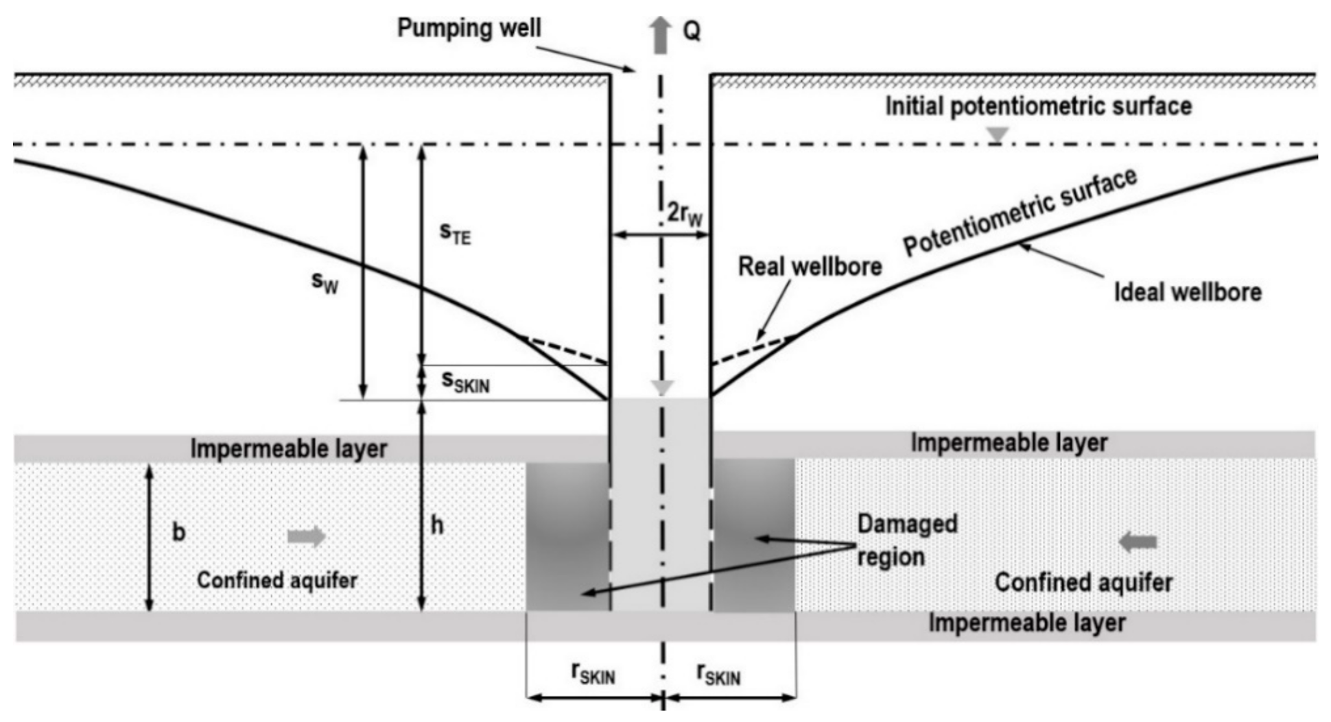
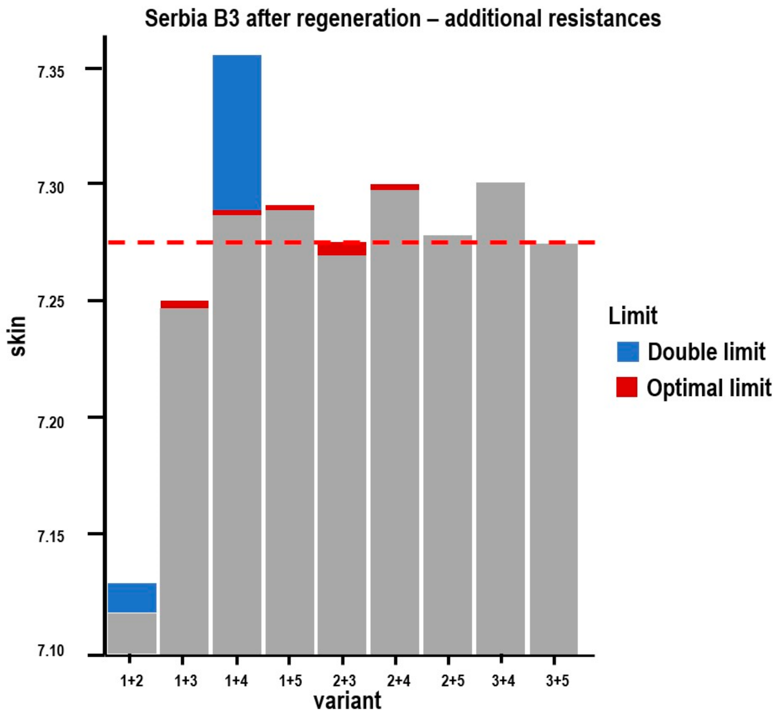
2.1. Additional Resistances (Skin Effect)
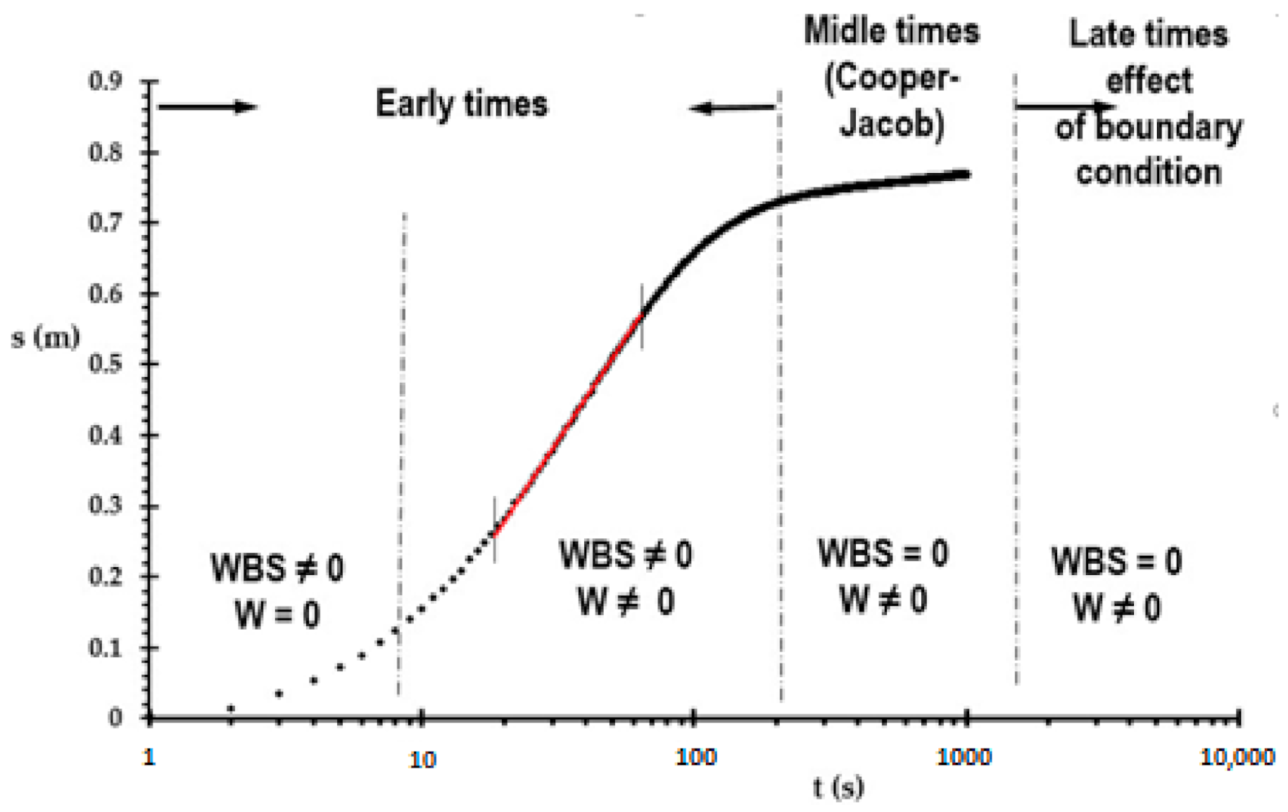
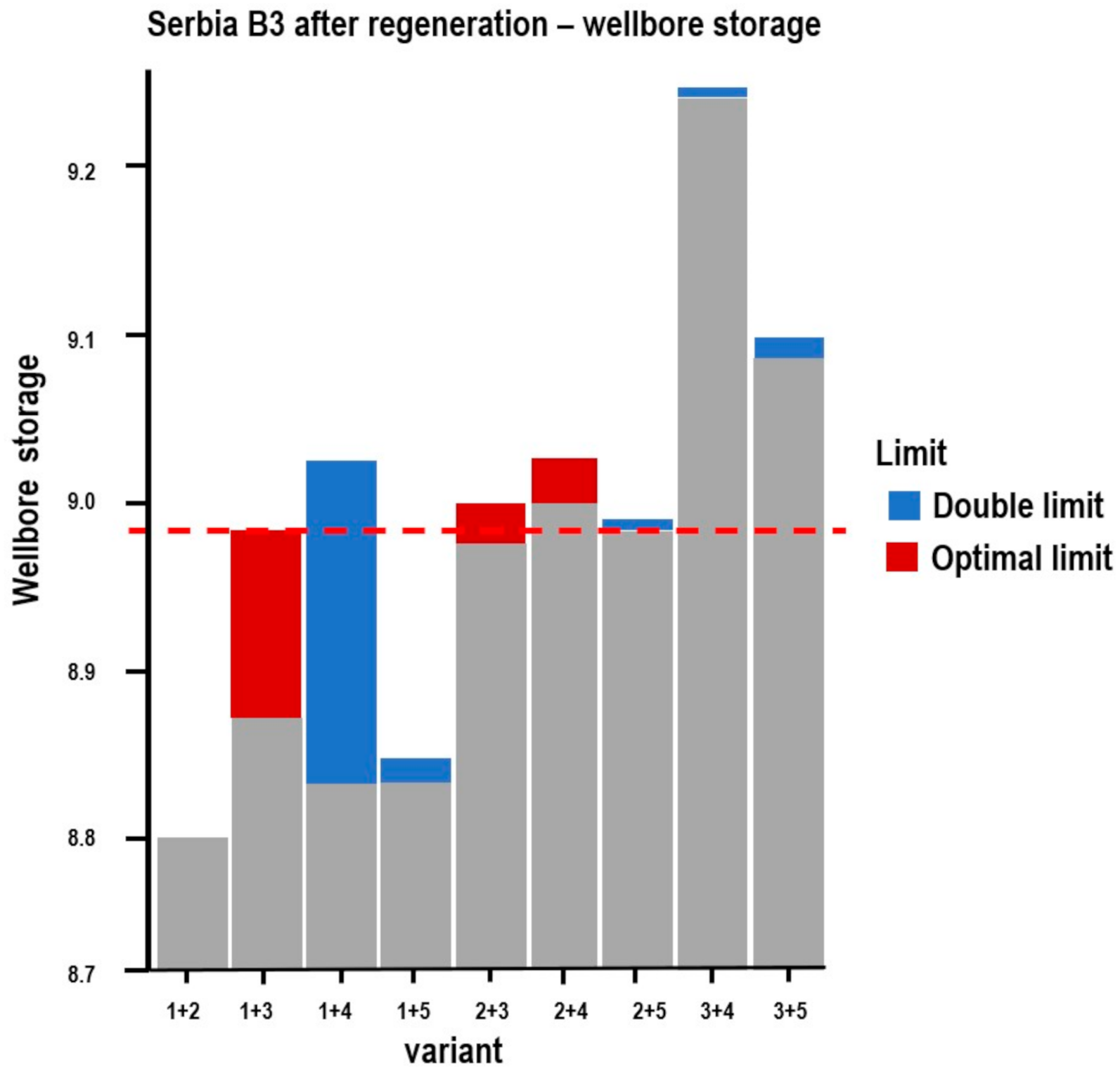
2.2. Well Storage (WBS)
- -
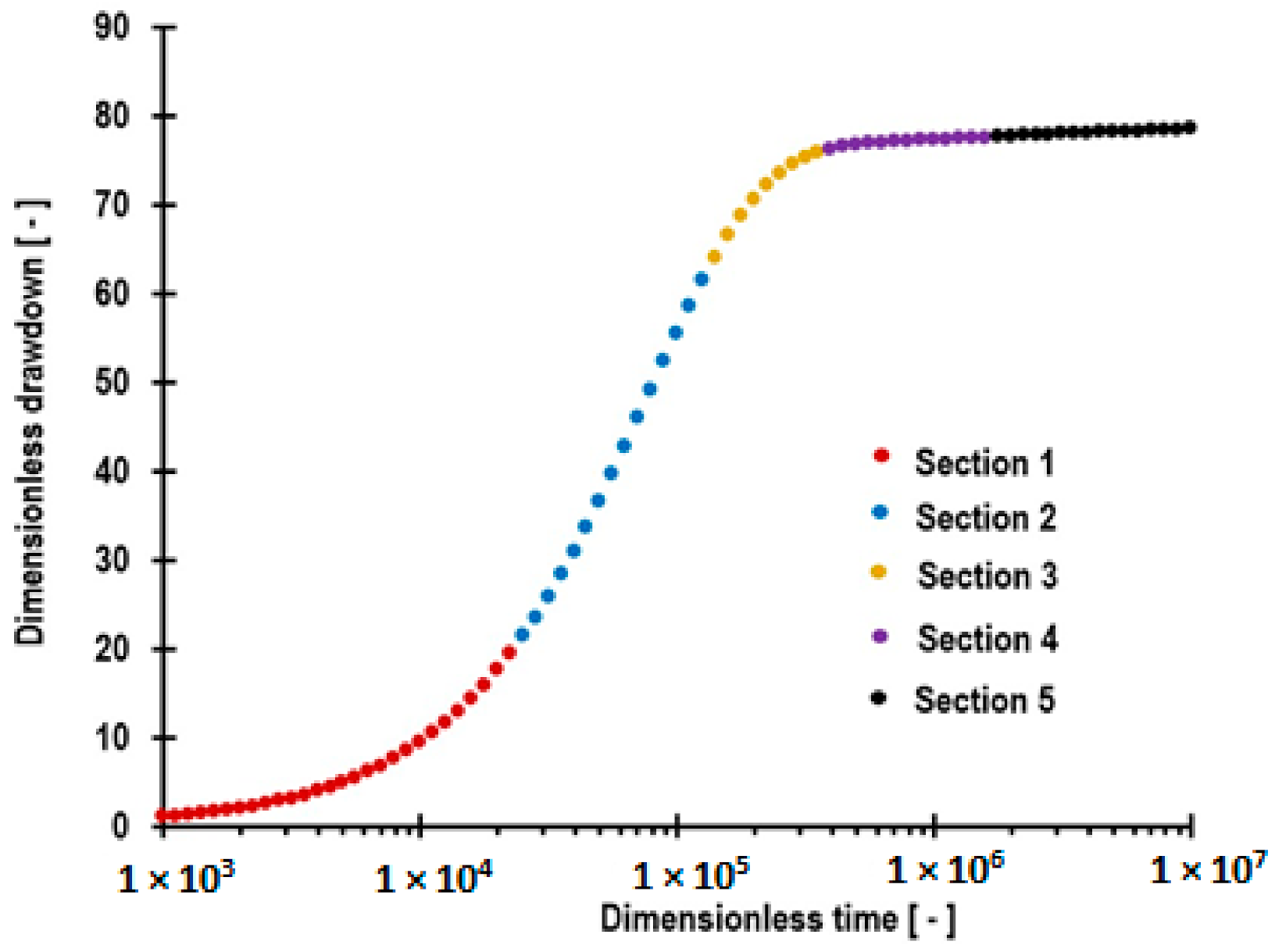
- Dimensionless time
- -
- Dimensionless radius
- -
- Dimensionless drawdown
- -
- Dimensionless drawdown at a well
- -
- Dimensionless well storagewhere r is the distance from the pumped well (m), H is the initial hydraulic head (m), h(r,t) is the hydraulic head at distance r and time t (m), and hw is the hydraulic head in the well (m).
- -
- The aquifer is confined and has a seemingly infinite areal extent.
- -
- The aquifer is homogeneous and isotropic and of uniform thickness over the area.
- -
- The flow is horizontal.
- -
- Prior to pumping, the piezometric surface is horizontal over the area.
- -
- The pumping rate is constant throughout the pumping test.
- -
- The well penetrates the entire thickness of the aquifer.
- -
- The well has a finite volume, and the well storage coefficient is constant throughout the pumping test.
- -
- Additional resistances in the well and its surroundings are non-zero.
3. Data
4. Results
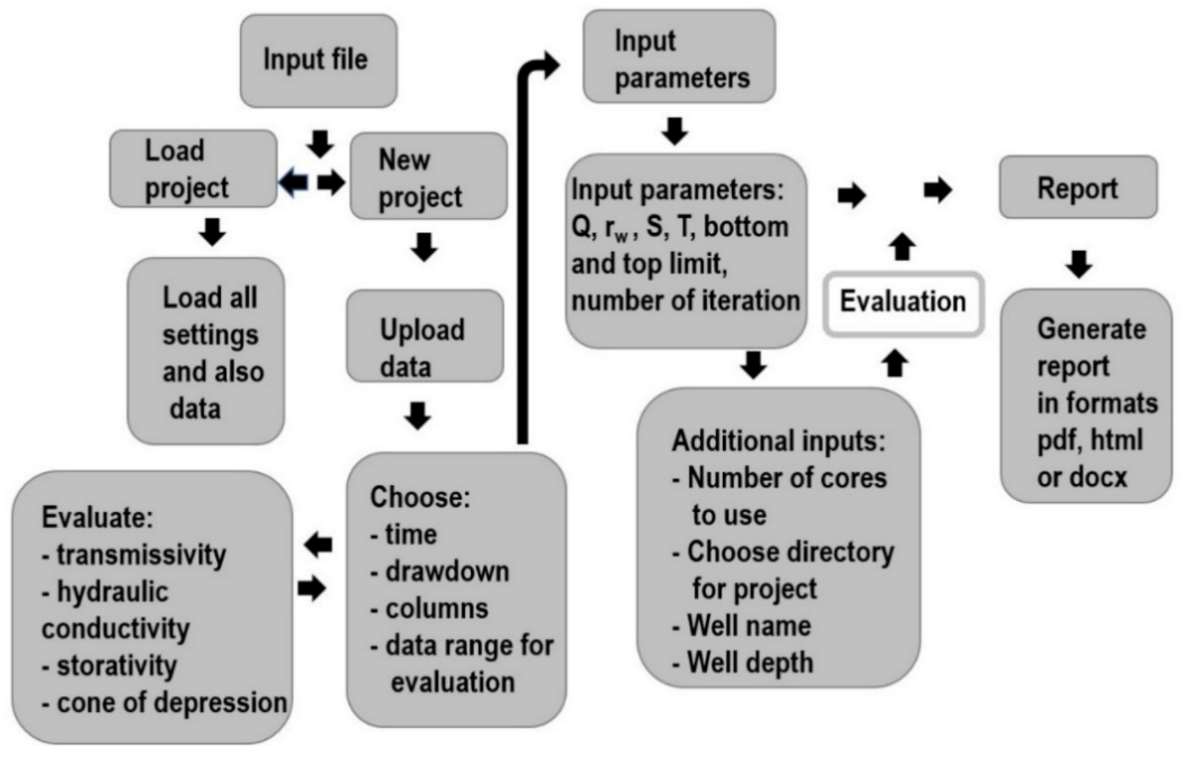
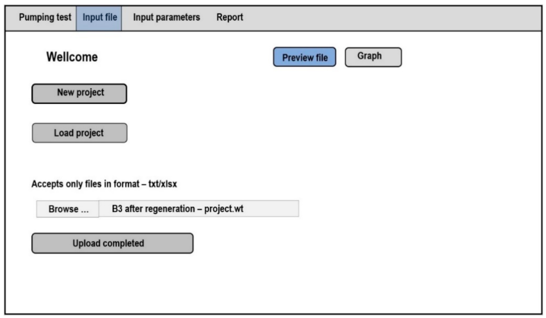
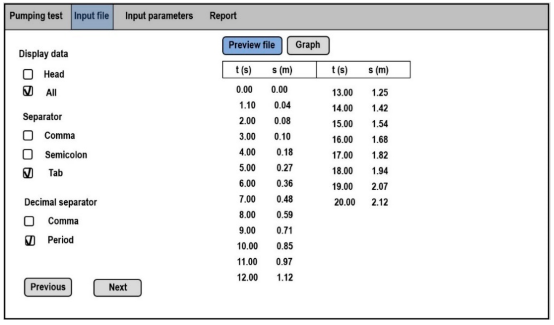
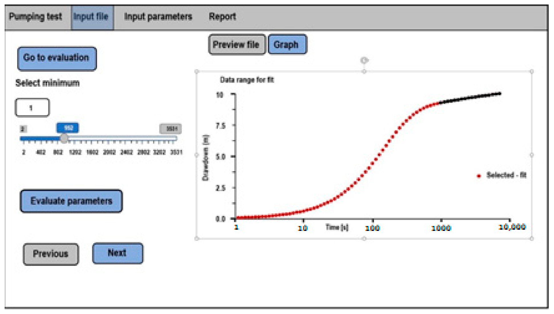
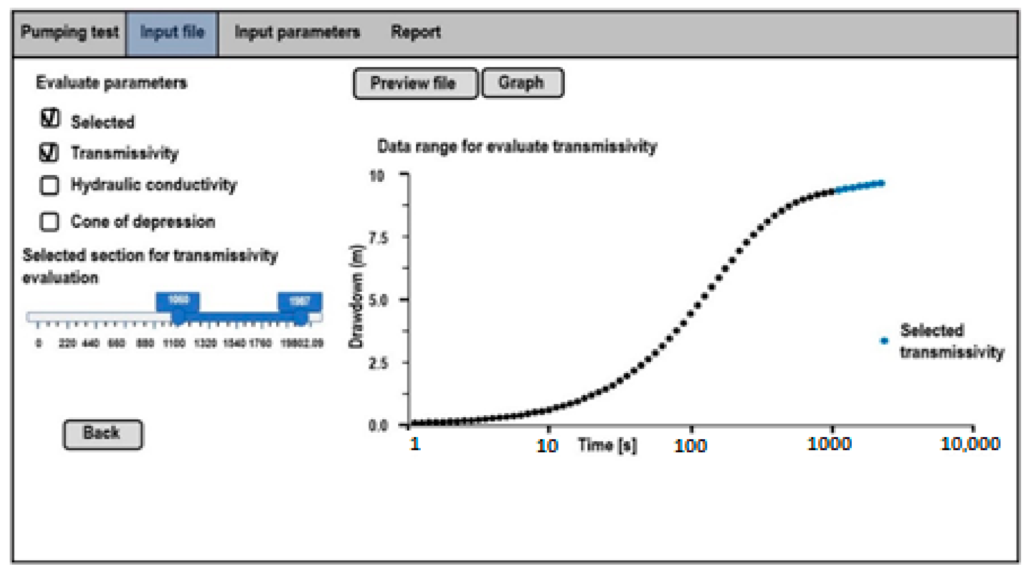
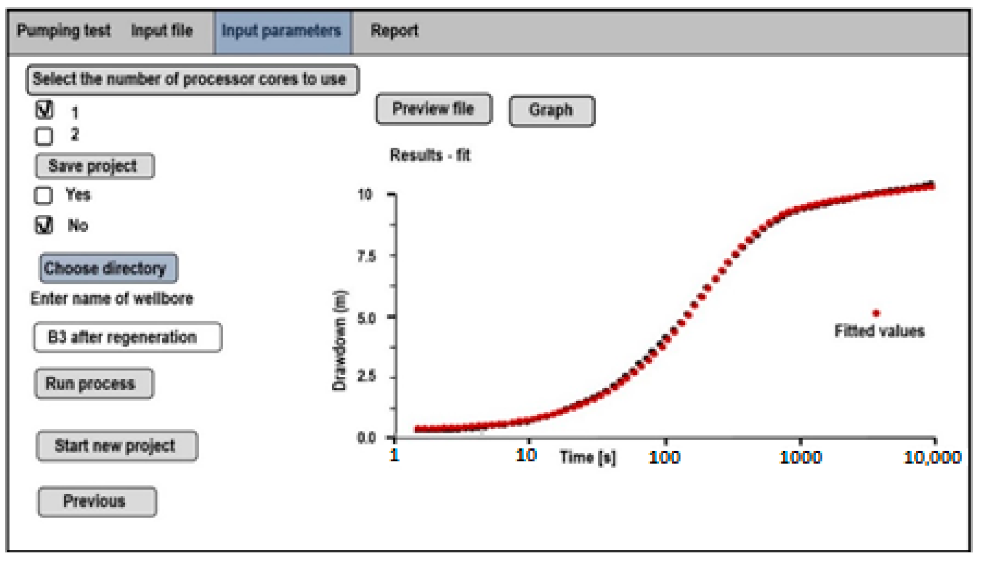
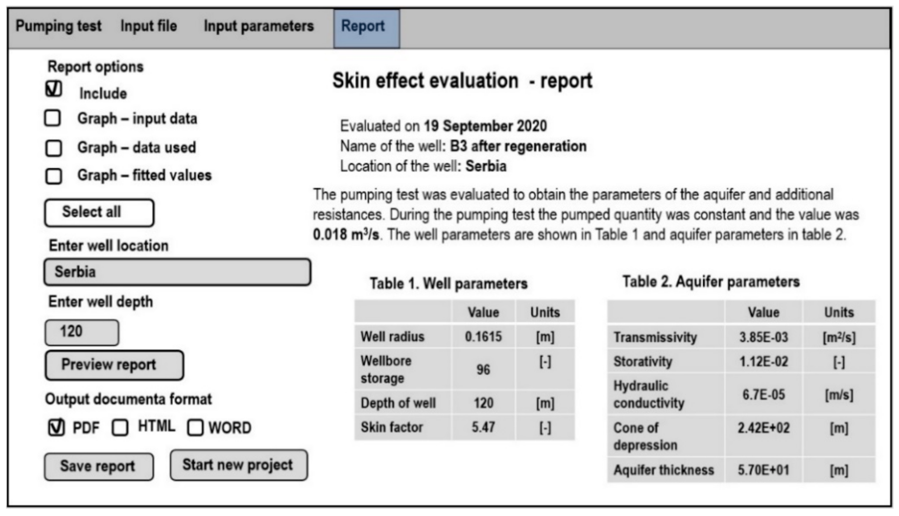
Software
5. Discussion
6. Conclusions
Author Contributions
Software
Funding
Institutional Review Board Statement
Informed Consent Statement
Data Availability Statement
Conflicts of Interest
References
- Theis, C.V. The relation between the lowering of the piezometric surface and the rate and duration of discharge of a well using ground-water storage. Trans. Am. Geophys. Union 1935, 16, 519–524. [Google Scholar] [CrossRef]
- Carslaw, H.S. Introduction to the Mathematical Theory of the Conduction of Heat in Solids; Macmillan and, Co.: London, UK, 1921; p. 286. [Google Scholar]
- Cooper, H.H.; Jacob, C.E. A generalized graphical method for evaluating formation constants and summarizing well-field history. Trans. Am. Geophys. Union 1946, 27, 526–534. [Google Scholar] [CrossRef]
- Van Everdingen, A.F. The skin effect and its influence on the productive capacity of a well. J. Pet. Technol. 1953, 5, 171–176. [Google Scholar] [CrossRef]
- Hurst, W. Establishment of skin effect and its impediment to fluid flow into a well bore. Pet. Eng. 1953, 25, B6–B16. [Google Scholar]
- Hawkins, M.F., Jr. A note on the skin effect. Trans. Am. Inst. Min. Metall. Eng. 1956, 8, 356–357. [Google Scholar] [CrossRef]
- Papadopulos, I.S.; Cooper, H.H. Drawdown in a well of large diameter. Water Resour. Res. 1967, 3, 241–244. [Google Scholar] [CrossRef]
- Ramey, H.J.; Agarwal, R.G. Annulus unloading rates as influenced by wellbore storage and skin effect. Soc. Pet. Eng. J. 1972, 12, 453–462. [Google Scholar] [CrossRef]
- Bourdet, D. Well test analysis: The use of advanced interpretation models. Handb. Pet. Explor. Prod. 2002, 3, 1–426. [Google Scholar] [CrossRef]
- Batu, V. Aquifer Hydraulics: A Comprehensive Guide to Hydrogeologic Data Analysis; John Wiley α Sons: New York, NY, USA, 1998; p. 727. ISBN 0-471-18502-7. [Google Scholar]
- Kucuk, F.; Brigham, W.E. Transient flow in elliptical systems. Soc. Pet. Eng. J. 1979, 19, 401–410. [Google Scholar] [CrossRef]
- Mathias, S.A.; Butler, A.P. Flow to a finite diameter well in a horizontally anisotropic aquifer with well storage. Water Resour. Res. 2007, 43, 1–6. [Google Scholar] [CrossRef]
- Yang, S.Y.; Yeh, H.D. Laplace-domain solutions for radial two-zone flow equations under the conditions of constant-head and partially penetrating well. J. Hydraul. Eng. ASCE 2005, 131, 209–216. [Google Scholar] [CrossRef]
- Chen, C.S.; Chang, C.C. Theoretical evaluation of non-uniform skin effect on aquifer response under constant rate pumping. J. Hydrol. 2006, 317, 190–201. [Google Scholar] [CrossRef]
- Yeh, H.D.; Yang, S.Y.; Peng, H.Y. A new closed-form solution for a radial two-layer drawdown equation for groundwater under constant-flux pumping in a finite-radius well. Adv. Water Resour. 2003, 26, 747–757. [Google Scholar] [CrossRef]
- Agarwal, R.G.; Al-Hussainy, R.; Ramey, H.J. An investigation of well storage and skin effect in unsteady liquid flow: I. Analytical treatment. Soc. Pet. Eng. J. 1970, 10, 279–291. [Google Scholar] [CrossRef]
- Wattenbarger, R.A.; Ramey, H.J. An investigation of well storage and skin effect in unsteady liquid flow: II. Finite difference treatment. Soc. Pet. Eng. J. 1970, 10, 291–297. [Google Scholar] [CrossRef]
- Kasenow, M. Determination of Hydraulic conductivity from Grain Size Analysis; Water Resources Publications LLC.: Carlton, CO, USA, 2010; p. 196. ISBN 978-1-887201-58-2. [Google Scholar]
- Gringarten, A.C.; Bourdet, D.P.; Landel, P.A.; Kniazeff, V.J. A comparison between different skin and well storage type-curves for early–time transient analysis. Soc. Pet. Eng. Spe. Ann. Techn. C Exh. 1979, 1–16. [Google Scholar] [CrossRef]
- Earlougher, R.C., Jr. Advances in well test analysis. In Monograph Series–Society of Petroleum Engineers of AIME; SPE International: Dallas, TX, USA, 1977; p. 264. [Google Scholar]
- Earlougher, R.C., Jr.; Kersch, K.H. Analysis of short-time transient test data by type- curve matching. J. Pet. Technol. 1974, 26, 793–800. [Google Scholar] [CrossRef]
- Novakowski, K.S. A Composite analytical model for analysis of pumping tests af fected by well bore storage and finite thickness skin. Water Resour. Res. 1989, 25, 1937–1946. [Google Scholar] [CrossRef]
- Chu, W.C.; Garcia-Rivera, J.; Raghavan, R. Analysis of interference test data influenced by well storage and skin at the flowing well. J. Pet. Technol. 1980, 32, 623–630. [Google Scholar] [CrossRef]
- Van Everdingen, A.F.; Hurst, W. The application of the Laplace transformation to flow problems in reservoirs. J. Pet. Technol. 1949, 1, 305–324. [Google Scholar] [CrossRef]
- Watlton, W.C. Aquifer Test Modeling, 1st ed.; CRC Press: Boca Ralton, FL, USA, 2007; p. 240. ISBN 978-1-4200-4292-4. [Google Scholar]
- Stehfest, H. Algorithm368: NumericalinversionofLaplacetransforms. Commun. ACM 1970, 13, 47–49. [Google Scholar] [CrossRef]
- Al-Ajmi, N.M.; Ahmadi, M.; Ozkan, E.; Kazemi, H. Numerical Inversion of Laplace Transforms in the Solution of Transient Flow Problems With Discontinuities. In Proceedings of the SPE Annual Technical Conference and Exhibition, Denver, CO, USA, 21–24 September 2008. [Google Scholar] [CrossRef]
- Yang, S.Y.; Yeh, H.D. Radial groundwater flow to a finite diameter well in a leaky confined aquifer with a finite-thickness skin. Hydrol. Process. 2009, 23, 3382–3390. [Google Scholar] [CrossRef]
- Hall, P.; Chen, J. Water Well and Aquifer Test Analysis; Water Resources Publication, LLC.: Carlton, CO, USA, 1996; p. 409. ISBN 0-918334-93-4. [Google Scholar]
- Pasandi, M.; Samani, N.; Barry, D.A. Effect of well and finite thickness skin on flow to a partially penetrating well in a phreatic aquifer. Adv. Water Resour. 2008, 31, 383–398. [Google Scholar] [CrossRef]
- Payne, F.; Quinnan, J.; Potter, S. Remediation Hydraulics; CRC Press: London, UK, 2008; p. 432. ISBN 978-0849372490. [Google Scholar]
- Hiscock, K.M.; Bense, V.F. Hydrogeology Principles and Practice; Wiley-Blackwell: River St, Hoboken, NJ, USA, 2014; p. 544. ISBN 978-0-470-65662-4. [Google Scholar]
- Chen, C.; Lan, C. A simple data analysis method for a pumping test with skin and well storage effect. Terr. Atmos. Ocean. Sci. 2009, 20, 557–562. [Google Scholar] [CrossRef]
- Kruseman, G.P.; de Ridder, N.A. Analysis and Evaluation of Pumping Test Data, 2nd ed.; IILRI: Wageningen, The Netherlands, 2008; pp. 1–372. [Google Scholar]
- Wen, Z.; Huang, H.G.; Zhan, H.B. Non-Darcian flow in a single confined vertical fracture toward a well. J. Hydrol. 2006, 330, 698–708. [Google Scholar] [CrossRef]
- Barua, G.; Bora, S.N. Hydraulics of a partially penetrating well with skin zone in a confined aquifer. Adv. Water Resour. 2010, 33, 1575–1587. [Google Scholar] [CrossRef]
- Kahuda, D.; Pech, P. A new method for evaluation of well rehabilitation from the early-portion of the pumping test. Water 2020, 12, 744. [Google Scholar] [CrossRef]
- Dastkhan, Z.; Zolalemin, A.; Razminia, K.; Parvizi, H. Minimization and Removal of Well Storage Effect by Direct Deconvolution of Well Test Data; SPE Reservoir Characterisation and Simulation C onference and Exhibition: Abu Dhabi, United Arab Emirates, 2015. [Google Scholar] [CrossRef]
- Sousa, E.P.; Barreto, A.B.; Peres, A.M. Analytical Treatment of Pressure-Transient Solutions for Gas Wells With Well Storage and Skin Effects by the Green’s Functions Method. SPE J. 2016, 21, 1858–1869. [Google Scholar] [CrossRef]
- Fan, Z.; Rarashar, R. Transient flow to a finite-radius well with well storage and skin effect in a poroelastic confined aquifer. Adv. Water Resour. 2020, 142, 103604. [Google Scholar] [CrossRef]
- Holub, J.; Pech, P.; Kuraz, M.; Maca, P.; Kahuda, D. Evaluation of a pumping test with skin effect and well storage on a confined aquifer in the Bela Crkva, Serbia. Int. J. Water 2019, 13, 1–11. [Google Scholar] [CrossRef]
- Liu, P.C.; Li, W.H.; Xia, J.; Jiao, Y.W.; Bie, A.F. Derivation and application of mathematical model for well test analysis with variable skin factor in hydrocarbon reservoirs. AIP Adv. 2016, 6. [Google Scholar] [CrossRef]
- Sethi, R. A dual-well step drawdown method for the estimation of linear and non-linear flow Parameters and well skin factor in confined aquifer systems. J. Hydrol. 2011, 400, 187–194. [Google Scholar] [CrossRef]
- Mashayekhizadeh, M.D.; Ghazanfari, M.H. The application of numerical Laplace in version methods for type curve development in well testing: A comparative study. Pet. Sci. Technol. 2011, 29, 695–707. [Google Scholar] [CrossRef]


| Name | Transmissivity T (m2s−1) | Storativity S (-) |
|---|---|---|
| B1 | 0.00585 | 0.013 |
| B3 | 0.00385 | 0.0123 |
| B6 | 0.0036 | 0.00864 |
| Name | rW (m) | Well Depth (m) | Well Storativity (-) |
|---|---|---|---|
| B1 | 0.149 | 87 | 996.6 |
| B3 | 0.1615 | 120 | 689.7 |
| B6 | 0.1615 | 110 | 2405.3 |
| Locality and Well Name | Q (m3s−1) | rW (m) | T (m−2s−1) | S (-) | CD (-) | W Software | W Cooper–Jacob Equation (3) | Percentage Divergence (%) |
|---|---|---|---|---|---|---|---|---|
| Serbia B-1 | 0.0102 | 0.1500 | 0.0058 | 0.0130 | 990 | 5.41 | 5.25 | 3 |
| Serbia B-3 | 0.0180 | 0.1615 | 0.0026 | 0.0441 | 50.0 | 5.45 | 5.29 | 3 |
| Serbia B-6 | 0.0118 | 0.0118 | 0.0036 | 0.0863 | 148 | 3.03 | 3.56 | 15 |
| Serbia EB-1 | 0.0122 | 0.1615 | 0.003 | 0.0023 | 2360 | 4.84 | 4.74 | 2 |
| Drnovec CV-2 | 0.0588 | 0.1625 | 0.00241 | 0.0011 | 900 | 1.01 | 0.95 | 6 |
| Radouň RD-1 | 0.019 | 0.15 | 0.0098 | 0.00066 | 160 | 1.6 | 1.45 | 9.4 |
| Radouň RD-2 | 0.142 | 0.15 | 0.00106 | 0.00018 | 180 | 2.66 | 2.68 | 1 |
| Kolín KV-2 | 0.0022 | 0.17 | 0.0245 | 0.076 | 16 | 5.72 | 5.17 | 10 |
| Kolín KV-9 | 0.00416 | 0.17 | 0.023 | 0.076 | 10 | 4.98 | 5.01 | 1 |
| Obrtka O9A | 0.0026 | 0.186 | 0.0234 | 0.00038 | 5500 | 7.2 | 7.31 | 1.5 |
| Obrtka O9B | 0.0097 | 0.125 | 0.00186 | 0.0419 | 160 | 7.21 | 5.23 | 27 |
| Synthetic Test | Q (m3s−1) | rW (m) | T (m−2s−1) | S (-) | CD (-) | W (-) | W Software | W Cooper–Jacob Equation (3) | Percentage Divergence (%) |
|---|---|---|---|---|---|---|---|---|---|
| Test 1 | 0.005 | 0.20 | 0.0120 | 0.010 | 100 | 10 | 9.998 | 9.97 | 0.24 |
| Test 2 | 0.003 | 0.25 | 0.0015 | 0.002 | 100,000 | 20 | 20.0003 | 19.99 | 0.0017 |
| Test 3 | 0.012 | 0.40 | 0.0030 | 0.0025 | 100,000 | 50 | 50.007 | 49.99 | 0.0141 |
Publisher’s Note: MDPI stays neutral with regard to jurisdictional claims in published maps and institutional affiliations. |
© 2021 by the authors. Licensee MDPI, Basel, Switzerland. This article is an open access article distributed under the terms and conditions of the Creative Commons Attribution (CC BY) license (https://creativecommons.org/licenses/by/4.0/).
Share and Cite
Ficaj, V.; Pech, P.; Kahuda, D. Software for Evaluating Pumping Tests on Real Wells. Appl. Sci. 2021, 11, 3182. https://doi.org/10.3390/app11073182
Ficaj V, Pech P, Kahuda D. Software for Evaluating Pumping Tests on Real Wells. Applied Sciences. 2021; 11(7):3182. https://doi.org/10.3390/app11073182
Chicago/Turabian StyleFicaj, Václav, Pavel Pech, and Daniel Kahuda. 2021. "Software for Evaluating Pumping Tests on Real Wells" Applied Sciences 11, no. 7: 3182. https://doi.org/10.3390/app11073182
APA StyleFicaj, V., Pech, P., & Kahuda, D. (2021). Software for Evaluating Pumping Tests on Real Wells. Applied Sciences, 11(7), 3182. https://doi.org/10.3390/app11073182