Article

Behavioral Modeling of Memristor-Based Rectifier Bridge

1
Department of Electrical Engineering Theory, Saint Petersburg Electrotechnical University “LETI”, 197376 St. Petersburg, Russia
2
Wuerth Elektronik eiSos GmbH, 74638 Waldenburg, Germany
*
Author to whom correspondence should be addressed.
Appl. Sci. 2021, 11(7), 2908; https://doi.org/10.3390/app11072908
Submission received: 3 March 2021 / Revised: 21 March 2021 / Accepted: 23 March 2021 / Published: 24 March 2021
(This article belongs to the Section Electrical, Electronics and Communications Engineering)

Abstract

:
In electrical engineering, radio engineering, robotics, computing, control systems, etc., a lot of nonlinear devices are synthesized on the basis of a nanoelement named memristor that possesses a number of useful properties, such as passivity, nonlinearity, high variability of parameters, nonvolatility, compactness. The efficiency of this electric element has led to the emergence of many memristor technologies based on different physical principles and, as a result, to the occurrence of different mathematical models describing these principles. A general approach to the modeling of memristive devices is represented. The essence is to construct a behavioral model that approximates nonlinear mapping of the input signal set into the output signal set. The polynomials of split signals, which are adaptive to the class of input signals, are used. This adaptation leads to the model’s simplification important in practice. Multi-dimensional polynomials of split signals are built for the rectifier bridge at harmonic input signals. The modeling error is estimated in the mean-square norm. It is shown that the accuracy of the modeling is increased in the case of using the piecewise polynomial with split signals.

1. Introduction

Recently, the element base for the designing of nonlinear dynamic devices is changed due to the emergence of elements with new properties and technologies for their creation. More and more devices are synthesized based on memristors or memristive structures [1,2,3,4]. This process results from the effective characteristics of a memristor as a passive electrotechnical element. The memristor possesses the following useful properties [1,2,3,4]:
  • Being an analog element, its resistance can take any values. This is a positive property in comparison with any binary element whose value can be either 0 or 1. Such variability of resistance is realized in one element, the memristor size is reduced to several nanometers and the response rate is reduced to nanoseconds.
  • The memristor does not store a charge. This means that it is not prone to charge leaks, which must be dealt with when going to nanometer-scale microcircuits.
  • The memristor is a non-volatile element, and data can be stored as long as the materials from which it is made exist.
  • Memristors placed on crossing conductors (crossbars) can be used to form densely packed memory.
  • Many memristor materials are compatible with complementary metal-oxide-semiconductor (CMOS) technology.
A memristor was theoretically described first by L. Chua in 1971 [5]. There were a lot of investigations devoted to elements with resistive switching [6,7,8,9,10,11] and only in 2008 the link between resistive switching and the theory of memristors was established in the Hewlett Packard (HP) laboratory [12]. In [12] the authors represented a variant of the ideal memristor model, which doesn’t completely describe any resistive switching element [13]. Nowadays, memristive systems lead to building non-volatile storage devices [14,15], self-adjusting analog-digital control devices [14,15], hardware security [16], in-memory computing [17], programmable logic systems [18,19], neuromorphic systems [20,21], image converters [22], different types of neural networks, for instance, multi-layer feedforward, radial basis, recurrent, cellular, convolutional, neuro-fuzzy networks [23,24,25,26], and, undoubtedly, analog devices for various purposes (oscillators, chaotic circuits, amplifiers with a variable coefficient, comparators, Schmitt trigger, rectifiers, etc.) [27,28,29]. The mentioned advantageous diversity of the application fields is caused by using different materials and technologies for designing of memristors. Memristors can be made of a metal-isolator-metal (MIM) sandwich based on transition metal oxides such as TiO2, NiO2, CuO, HfO2, etc. These memristors are called resistive ones due to the capability of resistance switching. In majority cases, other memristors are fabricated as spintronic, organic (polymeric) and ferroelectric ones [30]. However, the mentioned aspect has a negative effect that consists in the great variety of mathematical memristor models. These models describe different physical processes in memristors. As a result, we have to face the challenge of using mathematical memristor models, which essentially depend on the specifics of materials and technologies. These difficulties emerge on modeling memristor-based devices too.
The way of overcoming the mentioned challenges is the modeling of memristors and memristor-based devices on the input/output approach, which proposes to build a behavioral model on using the assigned sets of the input and output signals of a device represented as a nonlinear dynamic system. According to this approach the device is considered to be a «black box» and we construct its general mathematical model without taking into account the internal parts of the device. This view is appropriate and effective when a general model cannot be synthesized by means of the component models (there is no sufficient description of the structure or components of the device), as well as when the device is a part of more complicated constructions. In the latter case, the application of the device’s behavioral model leads to simpler representations of constructions composed of many different devices. A behavioral model approximates an operator that uniquely maps the domain of the input signals into the domain of the output signals of a nonlinear dynamic system [31,32,33,34]. As a rule, the approximation problem is solved in the mean-square norm on building universal mathematical models. Among behavioral models, we can distinguish the Volterra series [31,32,33,34], multi-dimensional split polynomial [35,36,37,38], numerous structures of regression models [39,40] and neural networks [41]. Multi-dimensional split polynomial is worth highlighting. This model obtains unique global optimum parameters resulting from approximating the operator of a nonlinear dynamic system in the mean-square norm that is superior to neural networks when we determine a lot of local optimum parameters. The structure of multi-dimensional split polynomial depends on a specific type of the input signal, therefore, this model is less universal but simpler in comparison with the Volterra polynomial. The model simplicity is preferable for the model implementation. Moreover, a feedforward structure of split polynomial is independent of keeping stable regime that is characteristic of feedback mostly relevant to regression models. Thus, multi-dimensional split polynomial has advantages over other mentioned models, which ensure its success in modeling of nonlinear dynamic systems including different memristor-based devices.
In this paper, multi-dimensional split polynomial is represented for modeling a rectifying memristor bridge. A rectifier bridge (the Graetz circuit, full-wave rectifier) is a popular device in electrotechnical and radio engineering. Generally, it is an intermediate circuit for converting alternating current (AC) signals into direct current (DC) signals. Modern electronics is mainly using DC voltage for operation, but the energy distribution network works on AC voltage. A diode rectifier feeding an ohmic-capacitive load is the input stage of many devices, which are connected to the distribution grid, such as battery chargers (including those for electric vehicles), computers, household appliances and many others [42]. A rectifier bridge can operate as a passive circuit using diodes or as an active circuit using bipolar junction transistors (BJTs) or field effect transistors (FETs). In any of these cases the current flow on the AC side is non-linear which causes higher order current harmonics. For mains powered devices the magnitude of these harmonics is to be limited [42]. An additional power factor correction (PFC) circuit is needed. The utilization of memristors instead of diodes for the rectifier bridge is a new investigation trend. Due to the nature of a physically realized memristor it is not yet usable for power electronic applications. In order to get an unidirectional valve effect for the current, as it is the case for the rectifier diode, a bipolar switching memristor is required and the operating frequency needs to be in the lower Hertz region [43,44]. For low power applications the memristor-based rectifier bridge can be used in synapse-based neural networks with programmable synaptic weights [45,46]. Another application is image processing; by adding a capacitor at the output of the memristive bridge embodies a low-pass filter with time-varying cut-off frequency and transfer function [47]. Thus, the use of memristors in the well-known Graetz circuit essentially expands its application. For investigation of memristor-based devices, both empirical models adapted from the ideal memristor model and models based on physical considerations [48,49,50,51,52,53] play an important role.

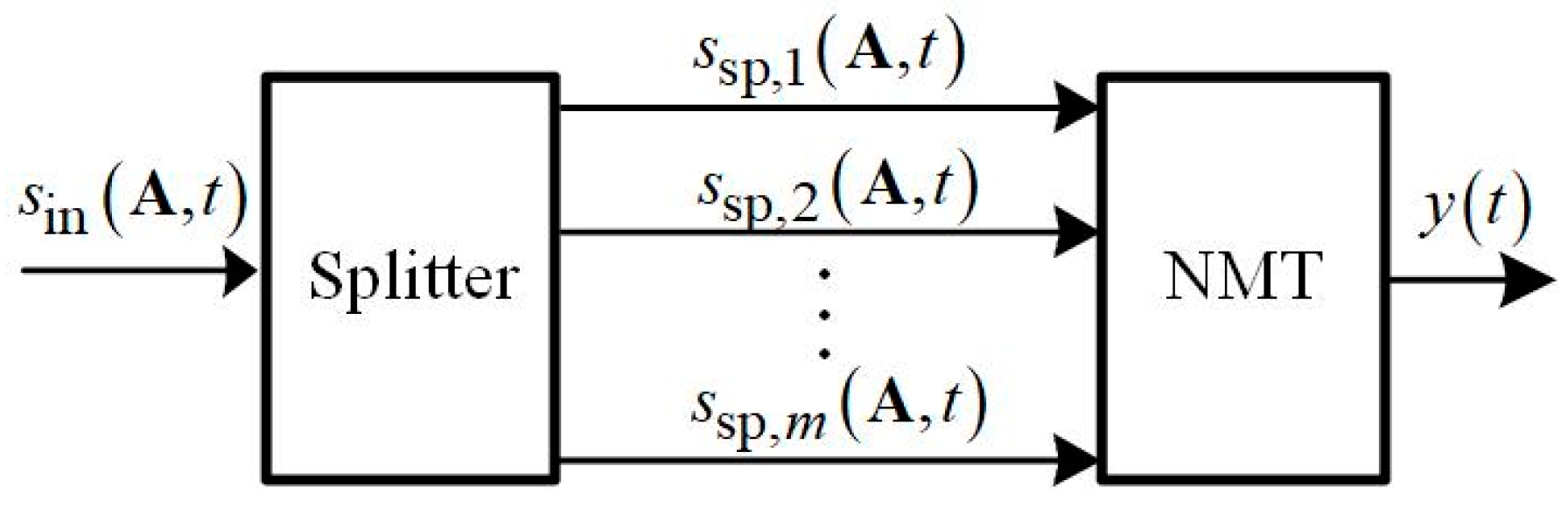
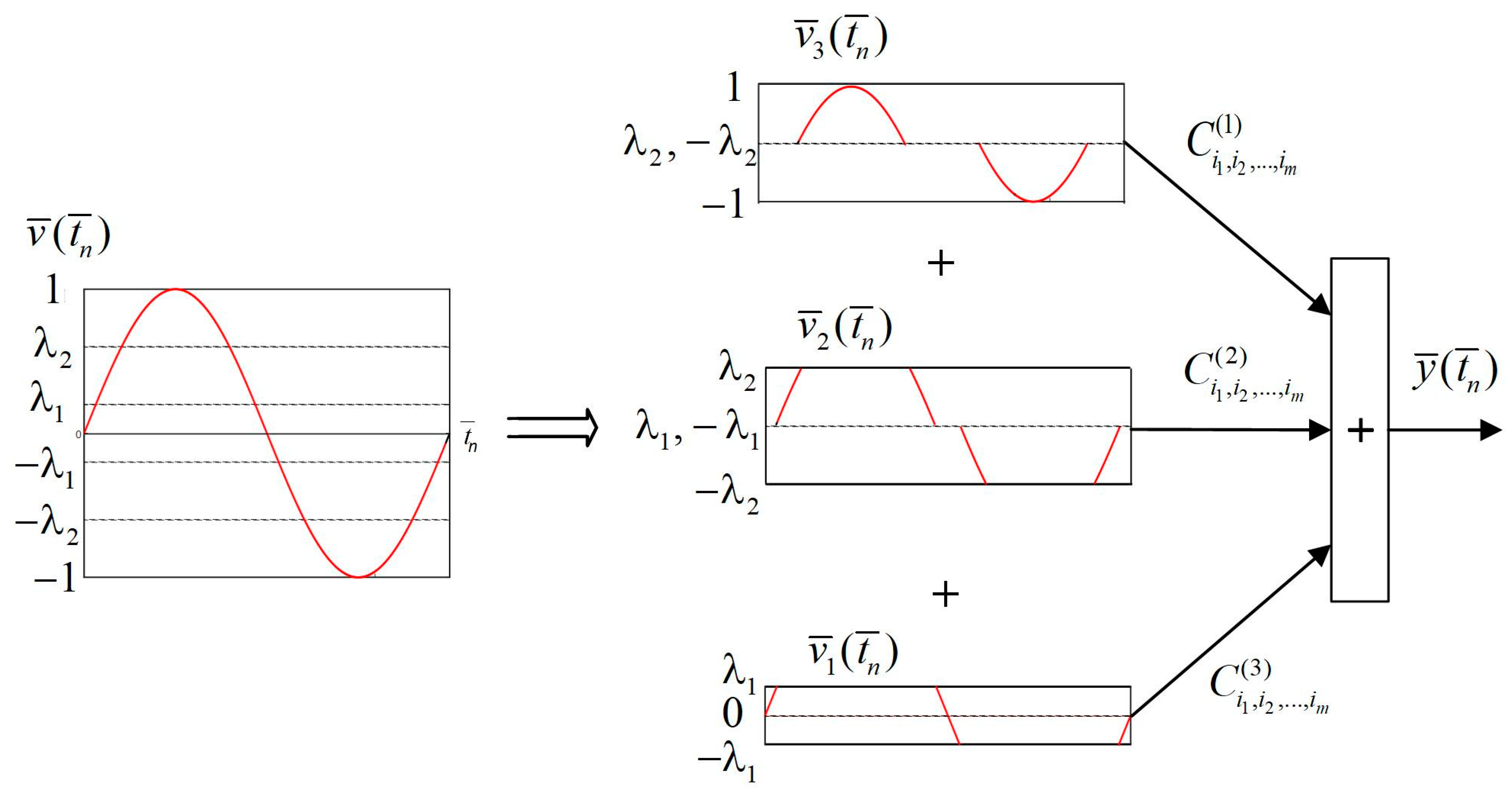
2. Multi-Dimensional Split Polynomial as a Behavioral Nonlinear Model

A split polynomial approximates the operator of a nonlinear system under an assigned error. This error is estimated in accordance with a norm. We take the well-known mean-square norm as the most popular in practice. The model maps the domain of the input signals into the corresponding domain of the output signals. The model parameters result from solving the following approximation task
s out o ( t ) s out ( t ) min C ,
where s out o ( t ) , s out ( t ) are the output signals of a nonlinear system and a model correspondingly; C is a vector of the model parameters. The solution of the optimization task (1) is determined on using the given sets of the input and output signals. This solution is global optimum in the case of linear-in-the-parameter model [31,32,33,34]. It encourages the popularity of polynomial models.
A designed split polynomial is to be unique, dynamic and nonlinear. The unique property means there is no mapping of one input signal into some output signals. The model block-scheme depicted in Figure 1 ensures the mentioned properties. The first block named Splitter transforms every scalar input signal s in ( A , t ) into the vector signal S sp ( A , t ) , named split signal:
S sp ( A , t ) = [ s sp , 1 ( A , t ) ,   s sp , 2 ( A , t ) ,   ,   s sp , m ( A , t ) ] ,
where A , A     G a is the parameters vector of the input signal s in ( A , t ) from the domain   G a of parameters;   t ,   t     G t is the time variable existing in the time domain G t .
The mentioned transformation is carried out according to the following conditions [35,36,37,38]:
  • for all A     G a , t     G t , there is an inequality
    S sp ( A , t ) 0 ;
  • for any A α A β , A α   G a , A β     G a , t α     t β , t α     G t , t β     G t , there is an inequality
    S sp ( A α , t α ) S sp ( A β , t β ) .
Equations (3) and (4) mathematically describe the situation, that the phase portraits, which are built on the axes of the elements of split vector (2), don’t cross and touch each other as well as don’t pass through zero. The splitter is a dynamic circuit that provides unique and dynamic properties of a model. Splitting signals can be implemented by linear and nonlinear, stationary and non-stationary dynamic circuits [35,36,37,38]. The main implementation criterion is, the lower the length of a split vector (2), the lower the dimensionality and consequently complexity of a model. The splitter depends on the input signal, since it splits the particular input signal. Therefore, one can say, the split model is adaptive to the input signal, thus it can be simpler in comparison with general polynomial, regression or neural models.
The splitter is followed by the block named Nonlinear Memoryless Transformer (NMT), that creates the model nonlinearity. The NMT transforms the split vector signal into the scalar output signal of a model. This nonlinearity can be described by a polynomial, a fraction and a regression, as well as neural networks. The most popular form is a polynomial, that is used for modeling in this paper. The polynomial is written
y ( t ) = j 1 = 0 J 1 j 2 = 0 J 2 j m = 0 J m C j 1 j 2 j m [ s sp , 1 ( A , t ) ]   j 1 [ s sp , 2 ( A , t ) ]   j 2 [ s sp , m ( A , t ) ]   j m .
The power of polynomial (5) equals J = r = 1 m J r . The elements of the split vector signal (2) form basis functions in (5), that is why the polynomial is multi-dimensional. The dimension of the model is the length of the split vector (2).
Further, we use the described split polynomial for the mathematical modeling of the memristor-based rectifier bridge. By simulating the rectifier bridge in the LTspice program, we obtain the sets of the input and output signals required for building this model. This program is famous for simulating a majority of analog circuits and it includes some of the well-known memristor models [43].

3. Forming the Sets of Input and Output Signals of the Memristor-Based Rectifier Bridge

The circuit of the memristor-based rectifier bridge simulated in LTspice is shown in Figure 2. A sinusoidal voltage source with variable amplitude A and frequency f acts as the excitation (the input signal). A simple 1 kΩ resistor acts as a load. The voltage of the resistive load is the output signal. At a positive half period of the sinusoidal input voltage, the memristance of the two P-xsv-N memristors (see Figure 2) is decreasing, while the memristance of the two N-xsv-P memristors is increasing until saturation is reached. At a negative half period of the input voltage the process is reversed. During one period there is a change of processes between both memristances. Thus, in the ideal case the output voltage is only positive, and this pulsed voltage has double the frequency of the input signal. In the real case there are the temporary short negative voltage-time areas in the output signal, due to the time shift in the state variable change. The circuit comprises memristors described by the Yakopcic model. The parameters of the Yakopcic model are represented in LTspice and have the following values: a 1   =   0 . 076   A , a 2   =   0 . 06   A , b   =   3   V 1 , x 0   =   0 . 001 , x p   =   0 . 15 , x n   =   0 . 25 , A p   =   0 . 1 , A n =   10 , V p   =   0 . 9   V , V n   =   0 . 2   V , α p   =   1 , α n   =   4 , η   =   1 [54,55]. The equations of the memristor model are implemented in a sub-circuit called memristor_yakopcic.sub. The Yakopcic model will be explained in detail below. The directives (.param and .tran) seen in Figure 2 are only used as an example.
For the investigation of the rectifier, we have set the input signal parameters to the amplitude/frequency pairs (12 V/1 Hz), (13 V/2 Hz), (14 V/3 Hz), (15 V/4 Hz) and (16 V/5 Hz). The time window for simulation was set depending on the frequency and the number of signal periods N p . We have chosen N p   =   3 in order to let startup transients settle. The LTspice output signal does not have equally spaced timestamps, as the program adjusts the time steps automatically dependent on the temporal derivative of the signal. Only the final period of the output voltage was kept for post-processing. For interpolation we used N s   =   2001 equally spaced samples. As a final step, all waveforms were normalized to the same angular frequency ω   =   6 π   rad . By this the different maxima and minima are aligned.

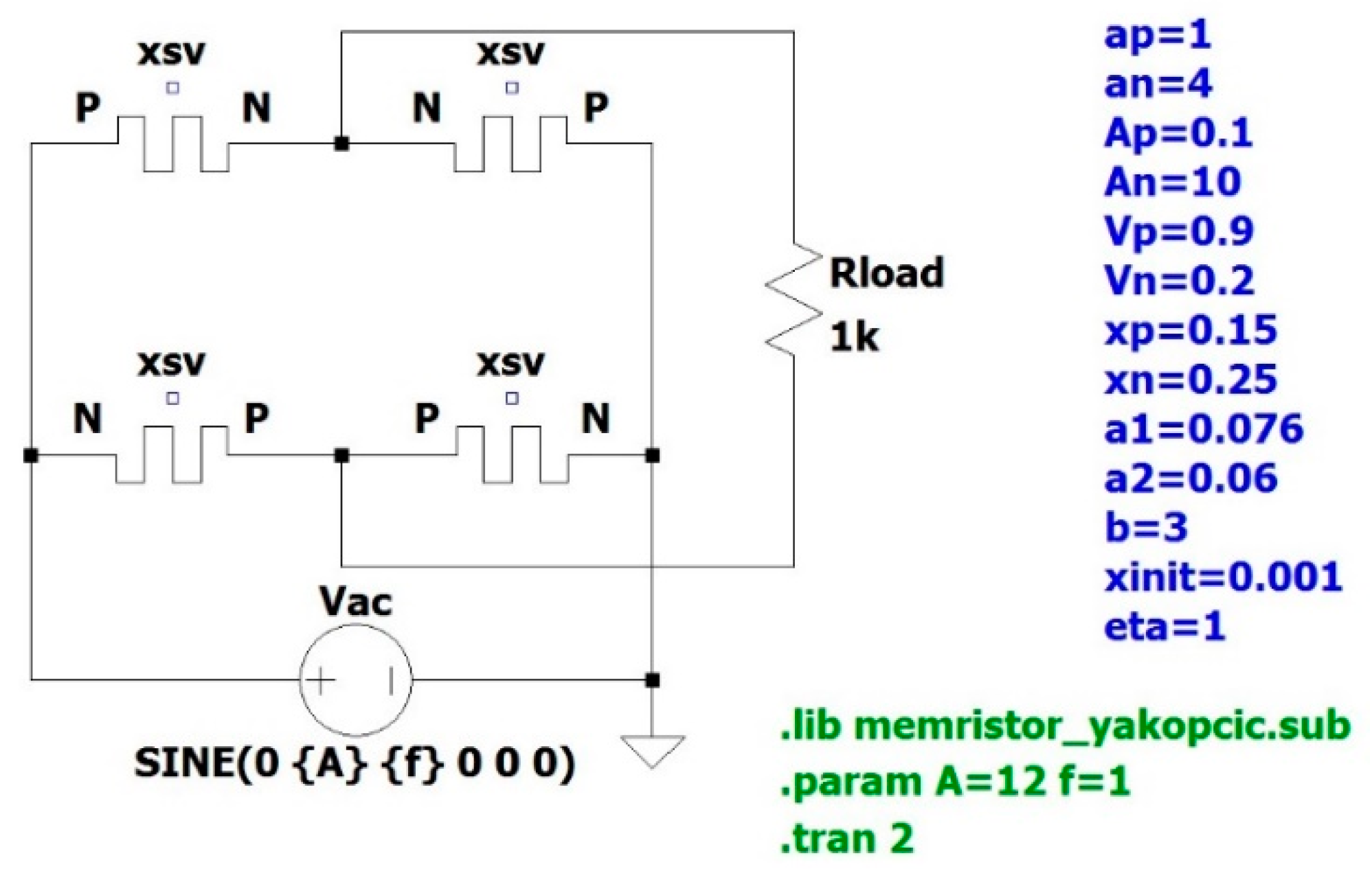
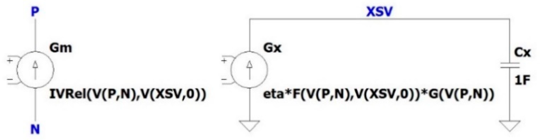
3.1. The Yakopcic Model of a Memristor in LTspice

The memristor model used in the circuit depicted in Figure 2 plays the important role for signal processing. In the past, several different mathematical memristor models were published; each of them aiming for a certain application. The first model was created by HP Laboratory in 2008 [12]. The basic current (I)–voltage (V) relationship can be found there. In 2009, the original HP model was extended by introducing the factor η , which describes the state variable motion with respect to the polarity of the applied voltage. Furthermore, a window function for the state variable motion was added [56]. The window function was modified by Biolek for a more realistic behavior of the state variable motion near the boundaries [57]. The first hardware related model was introduced by the Air Force Research Lab [58]. It does not use a state variable; the resistance change rate was defined directly. Later, models were implemented that describe a hyperbolic sine I–V relationship, like the one by the University of Michigan [59]. Previous models could only emulate sinusoidal input signal correctly, not general signal shapes. The hyperbolic sine model can approximate the I–V relationship of the MIM junction better.
For the implementation of a memristor model in LTspice we use the generalized hyperbolic sine model by Yakopcic et al. [55]. In comparison with the above-mentioned memristor models, the Yakopcic model uses more general equations for the memristor dynamics. Via fitting parameters, the model can be adapted to a variety of published memristor devices. The LTspice schematic of the sub-circuit can be seen in Figure 3.
The I–V relationship of the generalized memristor model depends on the state variable x ( t ) . Due to the MIM sandwich structure the memristive device shows an increase in conductivity beyond a certain voltage threshold. This behavior is considered by using a hyperbolic sine function.
i ( t ) = { a 1 x ( t ) sinh ( b v ( t ) ) v ( t ) 0 a 2 x ( t ) sinh ( b v ( t ) ) v ( t ) < 0 ,
where a 1 , a 2 and b are the parameters used to fit the model function to real memristive devices. The state variable x ( t ) is related to the resistance of the device, i.e., the relation of the length of the doped region to the overall length l d / l mem . In the LTspice sub-circuit, the state variable is named XSV. For the LTspice netlist Equation (6) is written as [55]
.func IVRel(V1,V2) = IF(V1 >= 0, a1*V2*sinh(b*V1), a2*V2*sinh(b*V1))
Here V1 stands for the voltage across the memristor v ( t ) and V2 stands for the state variable x ( t ) . The state variable change is described in (7) by two functions f ( x ( t ) ) and g ( v ( t ) ) :
d x ( t ) d t = η g ( v ( t ) ) f ( x ( t ) ) ,
where η is a factor which can be +1 or −1. It represents the direction of the motion of the state variable relative to the polarity of v ( t ) .
In order to get the derivative of the state variable, one can use a 1F capacitor in LTspice (Figure 3). Then the derivative of the node voltage V(XSV) is proportional to the current i x ( t ) in the capacitor which is equal to the current of the voltage dependent source Gx. Eventually, we can write:
d x ( t ) d t = 1 C i x ( t ) .
The initial state x 0 can be thought of as the voltage across the capacitor v C ( t = 0 ) [55]:
  • Cx XSV 0 {1}
  • .ic V(XSV) = xo
In order to change the state variable, a certain voltage threshold must be exceeded. The function g ( v ( t ) ) accounts for this behavior:
g ( v ( t ) ) = { A p ( e v ( t ) e V p ) v ( t ) > V p A n ( e v ( t ) e V n ) v ( t ) < V n 0 V n v ( t ) V p ,
where V p and V n are the positive and negative voltage thresholds; A p and A n are multipliers for state variable motion intensity in positive and negative direction.
The netlist implementation is as follows [55]:
.func G(V) = IF(V <= Vp, IF(V >= −Vn,0,−An*(exp(−V)−exp(Vn))),Ap*(exp(V)−exp(Vp)))
It is harder to change the state variable as it approaches the boundaries. This behavior is modeled by the second function f ( x ( t ) ) ,
f ( x ( t ) ) = { e α p ( x ( t ) x p ) w p ( x ( t ) , x p ) x ( t ) x p e α n ( x ( t ) + x n 1 ) w n ( x ( t ) , x n ) x ( t ) 1 x n 1 x ( t ) < x p x ( t ) > 1 x n ,
where x p and x n are the points at which the state variable motion is reduced; α p and α n are the rate in positive and negative direction, at which the state variable motion decays.
To assure that f ( x ( t ) ) approaches zero when x ( t )   =   1 , this function includes two window functions:
w p ( x , x p ) = x p x 1 x p + 1 ,
w n ( x , x n ) = x 1 x n .
These functions are written into the sub-circuit netlist as [55]
  • .func F(V1,V2) = IF(eta*V1 >= 0, IF(V2 >= xp,exp(−alphap*(V2−xp))*wp(V2),1), IF(V2 <= (1−xn), exp(alphan*(V2+xn−1))*wn(V2),1))
  • .func wp(V) = (xp−V)/(1−xp) + 1
  • .func wn(V) = V/(1−xn)
To complete the sub-circuit netlist, the voltage dependent current sources Gx and Gm get the values [55]
  • Gx 0 XSV value = {eta*F(V(P,N),V(XSV,0))*G(V(P,N))}
  • Gm P N value = {IVRel(V(P,N),V(XSV,0))}
Next, we describe the generation of input and output signals for the behavioral modeling of the memristor-based rectifier bridge.

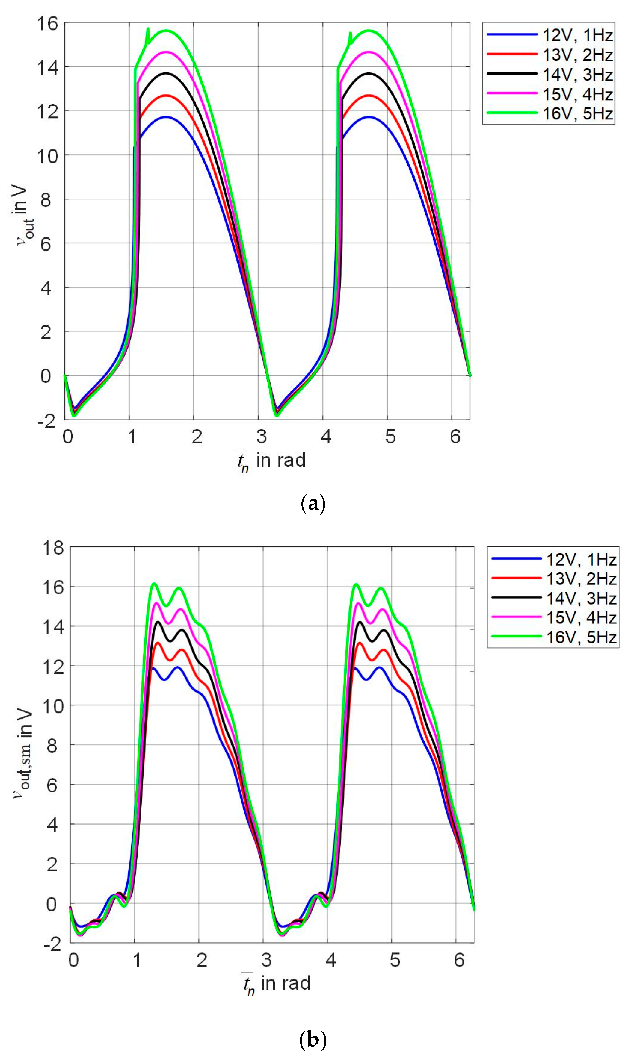
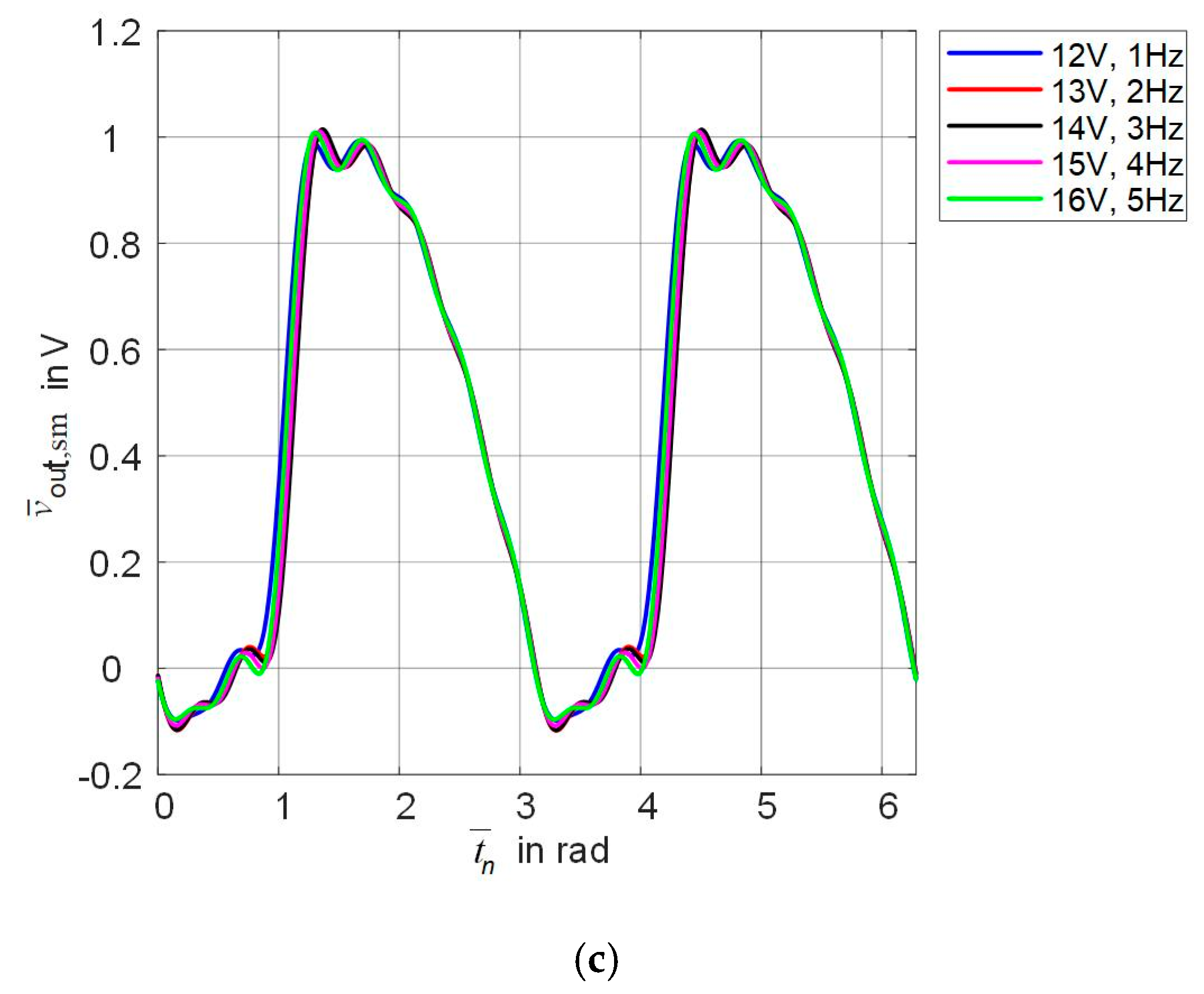
3.2. Smoothing Output Signals of the Memristor-Based Rectifier Bridge

To construct polynomial models, the set of the test input signals of the rectifier and the corresponding set of the output signals are formed. The harmonic input signal is written
v ( t ) = A sin ( ω 0 t ) ,
where A is an amplitude; ω 0 = 2 π f 0 is an angular frequency; f 0 is a frequency; t     [ 0 ,   T ) is time interval on a signal period; T is a signal period.
The set of the test input signals is generated on specifying the following vectors of amplitude and frequency:
A = [ 12 ; 13 ; 14 ; 15 ; 16 ]   V ,
F 0 = [ 1 ; 2 ; 3 ; 4 ; 5 ]   Hz ,
where A and F 0 are the amplitude and frequency vectors of the harmonic test exciters. The set of the corresponding output signals results from simulating the circuit shown in Figure 4. To build the mathematical models (a split polynomial), the number N p   =   2001 · 5 = 10,005 of the input-output pairs is used.
We use high amplitudes (9) of the input signal (8), since the rectifier bridge model based on the Yakopcic model of a memristor is severely nonlinear and the Yakopcic model requires high nonlinearity. With the given set of parameters this nonlinearity is achieved at high input amplitudes. One of our targets is to compare the split multi-dimensional polynomial of the rectifier bridge with the model based on the Yakopcic memristor model. It is well known that the memristor resistance can change for smaller voltages, leading to the so-called voltage-time dilemma and the resistance may degrade even at zero voltage [60]. It should be pointed out that the investigated “black box” approach is independent of the mentioned problem, since a behavioral model does not take the memristor model into account.
The input and output signals are sampled and normalized according to equation
ω 0 t n = 2 π f 0 t n = 2 π t n / T = t ¯ n ,
where t n ,   t n     [ 0 ,   T ) is a time sample; N = 2001 is the number of the time samples on the signal period; t n = ( n 1 ) T / ( N 1 ) ,   n   =   1 ,   2 ,   ,   N ;   t ¯ n ,   t ¯ n     [ 0 ,   2 π ) is a time-normalized sample; t ¯ n   =   2 π · ( n 1 ) / ( N 1 ) . Thus, when the frequency of the input signal (8) changes according to the vector F 0 from expression (10), we always have the time-normalized range t ¯ n     [ 0 ,   2 π ) . The rectifier outputs v out ( t ) are also converted to the time-normalized signals v out ( t ¯ n ) .
The time-normalized output signals of the rectifier at the excitation (8), in which the amplitude and frequency are assigned by the combination of elements from vectors (9) and (10), are shown in Figure 4a. As seen from Figure 4a, the output signals of the rectifier simulated with the Yakopcic model of memristors are not smooth functions. Every output signal has a point similar to discontinuity. This discontinuity is known to be generated by high-frequency harmonic components. To smooth signals, a low-pass filter, connected at the output of the rectifier, is used. Let’s apply an ideal low-pass filter. We simulate the filter action as follows. Each output signal of the rectifier is processed with the discrete Fourier transform of length N = 2001 . We keep the first 15 harmonics and zero the remaining ones. Then, we carry out the inverse discrete Fourier transform. As a result, the rectifier outputs are smoothed out. Figure 4b shows signals smoothed in comparison with those which are depicted in Figure 4a. It should be pointed out that the spectrum of the rectifier output signals contains even harmonics, since the nonlinear operator of a full-wave rectifier is even. This nonlinear operator transforms the harmonic input signal (8) into a polyharmonic one comprising only even harmonics.
Besides normalizing the time variable, the amplitude of the input signals is normalized
v ¯ ( t ¯ n ) = A sin ( t ¯ n ) / A = sin ( t ¯ n ) ,
where v ¯ ( t ¯ n ) is the discrete input signal with the normalized variables of time and amplitude, v ¯ ( t ¯ n )     [ 0 ,   1 ] ;   t ¯ n     [ 0 ,   2 π ) . Moreover, the amplitude of the output signals is normalized
v ¯ out , sm ( t ¯ n ) = v out , sm ( t ¯ n ) / A ,
where A is the amplitude of the harmonic input signal (8). The amplitude normalization is effective to compare the results obtained by different models. Figure 4c shows the smoothed signals with the amplitude- and time-normalized variables.

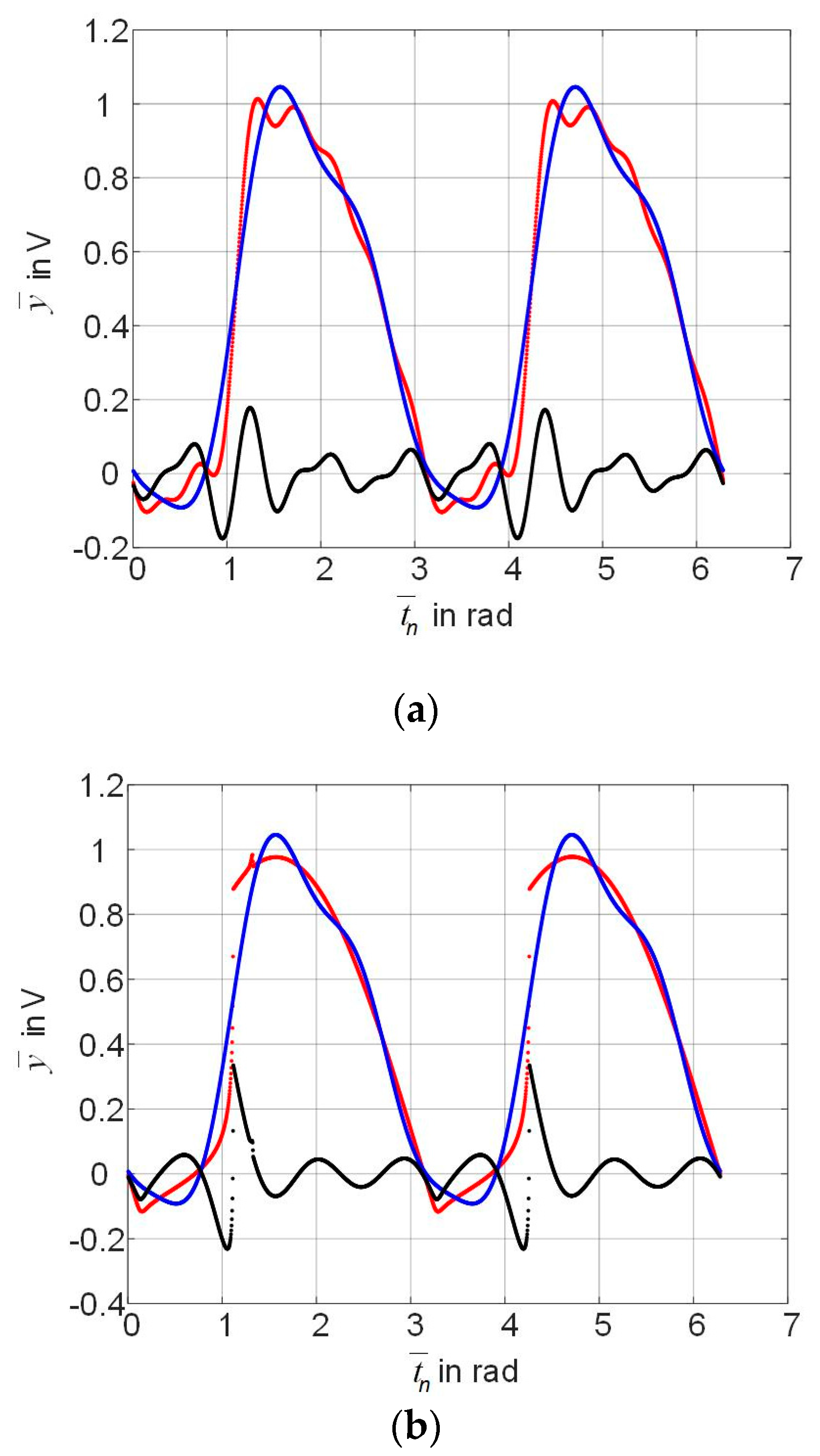
4. Results of the Rectifier Modeling Based on Multi-Dimensional Polynomials

The rectifier polynomial describes the mapping between the input signals set and the set of the smoothed rectifier output signals. The rectifier models are two-dimensional polynomials of different powers. Note there are the polynomials of the even-only degree, since the full-wave rectifier is described by an even operator. The two-dimensional polynomial of the 6th degree (the number of parameters is 15) is used as an example. The polynomial is of the form
y ¯ ( t ¯ n ) = m = 2 L i 1 = 0 I 1 i 2 = i 1 I 2 i m = i m 1 I m C i 1 i 2 i m v ¯ ( t ¯ n t ¯ i 1 ) v ¯ ( t ¯ n t ¯ i 2 ) v ¯ ( t ¯ n t ¯ i m ) ,
where C i 1 i 2 i m are the model parameters; L is the even power of the polynomial; m is an even degree; I 1 = I 2 = = I m = 1 are constants that determine the dimension of the polynomial in the corresponding coordinates. As the analysis of expression (11) shows, the presented polynomial is two-dimensional for any degree, its basis functions are the samples of the input signal at the current and previous time instants.
The model parameters result from solving the optimization problem:
v ¯ out , sm ( t ¯ n ) y ¯ ( t ¯ n ) min C ,
where v ¯ out , sm ( t ¯ n ) is discrete amplitude and time-normalized smoothed rectifier output signal, C is a vector containing the parameters of the model (8).
To estimate the accuracy of the constructed polynomials, three test input signals ( k = 1 ,   2 ,   3 ) were used, specified by expression (8) at amplitudes and frequencies from Table 1, and we calculated the following:
  • the uniform error
    Δ ¯ k ( t ¯ n ) = v ¯ out , sm , k ( t ¯ n ) y ¯ k ( t ¯ n ) ,   n = 1 , 2 , , 2001 ,   k = 1 , 2 , 3 ;
  • the maximum absolute error
    max ( | Δ ¯ ( t ¯ n ) | ) = max k = 1 , 2 , 3 ( max ( | Δ ¯ k ( t ¯ n ) | ) ) ,
    max ( | Δ ¯ k ( t ¯ n ) | ) = max t ¯ n ( 0 , 2 π ) ( | v ¯ out , sm , k ( t ¯ n ) y ¯ k ( t ¯ n ) | ) ,   n = 1 , 2 , , 2001 ;
  • the root-mean-square error
    ε k = 1 N 1 q = 1 N 1 ( v ¯ out , sm ( t ¯ q ) y ¯ k ( t ¯ q ) ) 2 ,   N = 2001 ,   k = 1 , 2 , 3 .
The maximum absolute and root-mean-square errors of modeling are represented in Table 1.
For the 3rd trial input signal, as shown in Figure 5a, the blue curve is the response y ¯ 3 ( t ¯ n ) of polynomial (11) of the 6th power, the red curve is the smoothed output signal v ¯ out , sm , 3 ( t ¯ n ) , the black curve is the uniform error Δ ¯ 3 ( t ¯ n ) from Equation (12) in the range t ¯ n     [ 0 , 2 π ) . Figure 5b shows correspondingly the response of the split polynomial, the non-smoothed load voltage v ¯ out , 3 ( t ¯ n ) , the uniform error obtained without smoothing by the low-pass filter. By comparing Figure 5a with Figure 5b, it can be seen that the non-smoothed output signal is described with a significantly greater error (black curve) than the smoothed output signal.
As follows from the analysis of Table 1 and Figure 5a,b, the higher the polynomial power, the higher the modeling accuracy. However, high-power polynomials are known to lead to ill-conditioned solutions when approximating a nonlinear operator; therefore, high-power polynomials are not constructive in practice. In this regard, we turn to piecewise polynomial models to achieve high modeling accuracy using the set of the low-power polynomials.

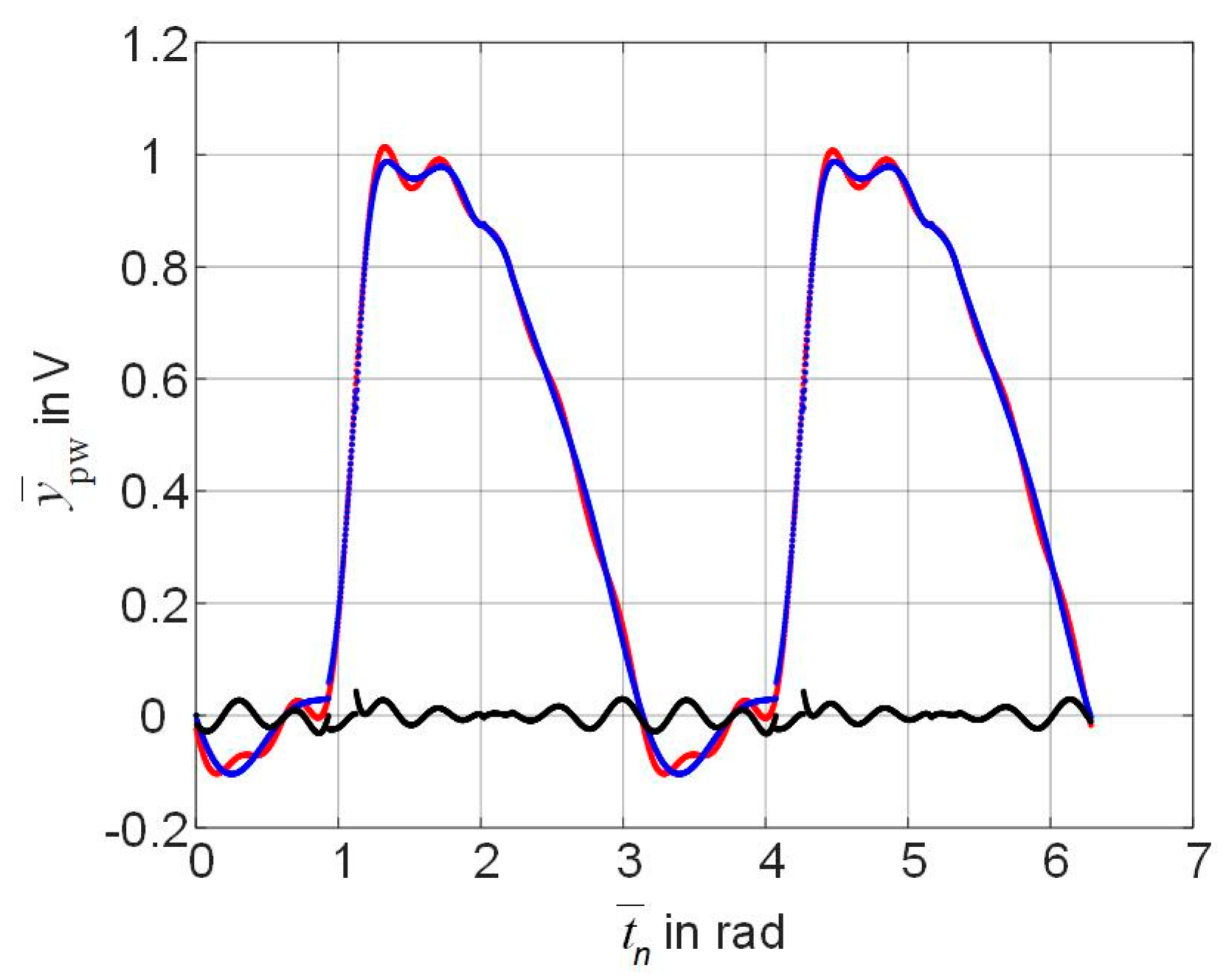
5. Results of the Rectifier Modeling Based on Piecewise Multi-Dimensional Polynomials

To construct a piecewise polynomial model of the rectifier, we divide the range of the normalized modulus of the input signal amplitude into several sub-ranges. The thresholds of the sub-ranges we denote as λ j 1 ; j = 1 , 2 , , J ; 0 < λ j 1 < 1 ; λ 0 = 0 ; λ J = 1 . The input sub-signals correspond to the mentioned amplitude sub-ranges, and every input signal is described by the sum
v ¯ ( t ¯ n ) = j = 1 J v ¯ ( j ) ( t ¯ n )
where v ¯ ( j ) ( t ¯ n ) is the input sub-signal with the normalized amplitude and time variables,
v ¯ ( j ) ( t ¯ n ) = { 0 | v ¯ ( j ) ( t ¯ n ) | λ j 1 | v ¯ ( t ¯ n ) | λ j 1 < | v ¯ ( j ) ( t ¯ n ) | λ j 0 | v ¯ ( j ) ( t ¯ n ) | > λ j
As a result, we form the sub-sets from the input sub-signals v ¯ ( j ) ( t ¯ n ) , t ¯ n [ 0 ,   2 π ) ,   j   =   1 ,   2 ,   ,   J . The sub-sets of the output sub-signals v ¯ out , sm ( j ) ( t ¯ n ) ,   t ¯ n [ 0 ,   2 π ) ,   j   =   1 ,   2 ,   ,   J correspond to the sub-sets of the input sub-signals.
The block-scheme of dividing the input signal into sub-signals according to the amplitudes and the formation of the response of the split piecewise-polynomial model is shown in Figure 6.
In the root-mean-square norm, using the sub-sets of the input sub-signals v ¯ ( j ) ( t ¯ n ) , t ¯ n [ 0 ,   2 π ) ,   j   =   1 ,   2 ,   ,   J . and the output sub-signals v ¯ out , sm ( j ) ( t ¯ n ) , we build models:
y ¯ pw ( j ) ( t ¯ n ) = m = 2 L i 1 = 0 I 1 i 2 = i 1 I 2 i m = i m 1 I m C i 1 i 2 i m ( j ) v ¯ ( j ) ( t ¯ n t ¯ i 1 ) v ¯ ( j ) ( t ¯ n t ¯ i 2 ) v ¯ ( j ) ( t ¯ n t ¯ i m )
where y ¯ pw ( j ) ( t ¯ n ) and C i 1 i 2 i m ( j ) ;   j   =   1 ,   2 ,   ,   J are the output sub-signals and parameters of the piecewise model on the sub-sets of the input signal respectively; L is the even power of the polynomial; m is an even degree.
The output signal of the piecewise model results from the following summation
y ¯ pw ( t ¯ n ) = j = 1 J y ¯ pw ( j ) ( t ¯ n )
where y ¯ pw ( j ) ( t ¯ n ) is described in (13).
Table 2 demonstrates the errors of modeling the memristive rectifier with the split piecewise-polynomial of the 6th power at three trial excitations. We used three sub-ranges of the normalized amplitude of the input signal, the thresholds of sub-ranges are λ 0   =   0 ,   λ 1   =   0 . 8 ,   λ 2   =   0 . 9 ,   λ 3   =   1 . The total number of the model parameters is 45.
As shown in Figure 7, the blue curve is the response of the polynomial (14) of the 6th power, the red curve is the smoothed output signal v ¯ out , sm , 3 ( t ¯ n ) of the circuit depicted in Figure 2, the black curve is the uniform error Δ ¯ 3 ( t ¯ n ) .
Comparison of the errors noted in Table 1 and Table 2, as well as in Figure 5a and Figure 7 results in the fact, that the piecewise-polynomial model ensures lower errors than a general polynomial model does.

6. Conclusions

Following previous research, we demonstrate the capabilities of the behavioral model in the form of the multi-dimensional split polynomial for the memristor-based rectifier bridge. This model describes the nonlinear input-output mapping of the device. The behavioral model is built with the help of the sets of the input and output signals which are calculated by the LTspice software. The rectifier bridge is represented as an electrical circuit with memristive elements described by the Yakopcic model at a harmonic excitation. For smoothing the output signals of the rectifier simulated in LTspice, an ideal low-pass filter is used. Then, both amplitude and time samples of the signals from the obtained input and output sets are normalized.
The behavioral model is represented as a multi-dimensional polynomial of split signals. The scalar input signal is converted to a vector by splitting. Further, the vector signal elements are used as base functions for constructing the multi-dimensional polynomial. The model parameters result from solving the approximation problem of a nonlinear rectifier operator in the mean-square norm. The advantages of the multi-dimensional split polynomial are as follows:
  • The form of the model and the method of its construction are universal, because they do not depend on the technology of memristor implementation.
  • Since a polynomial is linear-in-parameters, these parameters are defined as globally optimal by solving the approximation problem.
  • The splitting property allows the polynomial to be adapted to the assigned signal class, hence to construct a simpler model than other behavioral models.
To improve the accuracy of the modeling, the power of the split multi-dimensional polynomial should be increased. However, this operation leads to the problem of poor condition of the approximation problem when finding the model parameters. Therefore, the split piecewise-polynomial model free of this problem is proposed. Moreover, the piecewise-polynomial model is useful under the switching variability in memristors. As a result, we observe a significant reduction in the error of the rectifier bridge modeling.
The memristor-based rectifier bridge relates to, so-called, imperfect uncertain dynamic systems [61,62], since its working conditions affect the device parameters, the threshold and switching effects, robustness, etc. and, eventually, the device behavior. Thus, we face the problem of control taking into account the device limits. This problem can be solved in the framework of the control paradigm of imperfect and uncertain dynamic systems to gain a satisfactory trade-off between behavior and performance of the device [61,62].

Author Contributions

Conceptualization, E.S.; methodology, E.S.; software, E.S. and S.S.; validation, E.S. and S.S.; formal analysis, E.S. and S.S.; investigation, E.S. and S.S.; resources, E.S.; data curation, E.S. and S.S.; writing—original draft preparation, E.S. and S.S.; writing—review and editing, E.S., S.S. and H.H.; visualization, E.S., S.S. and H.H.; supervision, E.S.; project administration, E.S.; funding acquisition, E.S. All authors have read and agreed to the published version of the manuscript.

Funding

This research received no external funding.

Institutional Review Board Statement

Not applicable.

Informed Consent Statement

Not applicable.

Data Availability Statement

Not applicable.

Conflicts of Interest

The authors declare no conflict of interest.

References

  1. Corinto, F.; Forti, M.; Chua, L.O. Nonlinear Circuits and Systems with Memristors: Nonlinear Dynamics and Analogue Computing via the Flux-Charge Analysis Method; Springer Nature Switzerland AG: Cham, Switzerland, 2021; p. 438. [Google Scholar]
  2. Mladenov, V. Advanced Memristor Modeling: Memristor Circuits and Networks; MDPI: Basel, Switzerland, 2019; p. 170. [Google Scholar]
  3. Rahma, F.; Muneam, S. Memristive Nonlinear Electronic Circuits: Dynamics, Synchronization and Applications; Springer Nature Switzerland AG: Cham, Switzerland, 2019; p. 98. [Google Scholar]
  4. Vaidyanathan, S.; Volos, C. Advances in Memristors, Memristive Devices and Systems; Springer International Publishing AG: Cham, Switzerland, 2017; p. 511. [Google Scholar]
  5. Chua, L.O. Memristor—The missing circuit element. IEEE Trans. Circuit Theory 1971, CT-18, 507–519. [Google Scholar] [CrossRef]
  6. Kund, M.; Beitel, G.; Pinnow, C.U.; Roehr, T.; Schumann, J.; Symanczyk, R.; Ufert, K.D.; Mueller, G. Conductive bridging RAM (CBRAM): An emerging non-volatile memory technology scalable to sub 20nm. In Proceedings of the IEEE International Electron Devices Meeting, Washington, DC, USA, 5 December 2005; pp. 754–757. [Google Scholar]
  7. Kozicki, M.N.; Yun, M.; Hilt, L.; Singh, A. Applications of programmable resistance changes in metal-doped chalcogenides. Electrochem. Soc. 1999, 298, 298–309. [Google Scholar]
  8. Terabe, K.; Hasegaw, T.; Nakayama, T.; Aono, M. Quantum point contact switch realized by solid electrochemical reaction. Riken Rev. 2001, 37, 7–8. [Google Scholar]
  9. Beck, A.; Bednorz, J.G.; Gerber, C.; Rossel, C.; Widmer, D. Reproducible switching effect in thin oxide films for memory applications. Appl. Phys. Lett. 2000, 77, 139–141. [Google Scholar] [CrossRef]
  10. Jeong, D.S.; Schroeder, H.; Waser, R. Impedance spectroscopy of TiO thin films showing resistive switching. Appl. Phys. Lett. 2006, 89, 082909. [Google Scholar] [CrossRef] [Green Version]
  11. Szot, K.; Speier, W.; Bihlmayer, G.; Waser, R. Switching the electrical resistance of individual dislocations in single-crystalline SrTiO. Nat. Mater. 2006, 5, 312–320. [Google Scholar] [CrossRef] [PubMed]
  12. Strukov, D.B.; Snider, G.S.; Stewart, D.R.; Williams, R.S. The missing memristor found. Nature 2008, 453, 80–83. [Google Scholar] [CrossRef]
  13. Linn, E.; Siemon, A.; Waser, R.; Menzel, S. Applicability of well-established memristive models for simulations of resistive switching devices. IEEE Trans. Circuits Syst. I Regul. Pap. 2014, 61, 2402–2410. [Google Scholar] [CrossRef] [Green Version]
  14. Vourkas, I.; Sirakoulis, G.C. Memristor-Based Nanoelectronic Computing Circuits and Architectures; Springer International Publishing: Cham, Switzerland, 2016; p. 241. [Google Scholar]
  15. Zheng, N.; Mazumder, P. Learning in Energy-Efficient Neuromorphic Computing: Algorithm and Architecture Co-Design; John Wiley & Sons Ltd: Hoboken, NJ, USA, 2020; p. 276. [Google Scholar]
  16. Gao, Y.; Ranasinghe, D.; Al-Sarawi, S. Memristive crypto primitive for building highly secure physical unclonable functions. Sci. Rep. 2015, 5, 1–14. [Google Scholar] [CrossRef] [Green Version]
  17. Reuben, J.; Pechmann, S. A Parallel-friendly majority gate to accelerate in-memory computation. In Proceedings of the 2020 IEEE 31st International Conference on Application-specific Systems, Architectures and Processors (ASAP), Manchester, UK, 6–8 July 2020; pp. 93–100. [Google Scholar]
  18. Maan, A.K.; Jayadevi, D.A.; James, A.P. A survey of memristive threshold logic circuits. IEEE Trans. Neural Netw. Learn. Syst. 2016, 28, 1734–1746. [Google Scholar] [CrossRef] [Green Version]
  19. Vourkas, I.; Sirakoulis, G.C. Emerging memristor-based logic circuit design approaches: A review. IEEE Circuits Syst. Mag. 2016, 16, 15–30. [Google Scholar] [CrossRef]
  20. Zhang, Y.; Wang, X.; Li, Y.; Friedman, E.G. Memristive model for synaptic circuits. IEEE Trans. Circuits Syst. II Express Briefs 2017, 64, 767–771. [Google Scholar] [CrossRef]
  21. Corinto, F.; Torcini, A. Nonlinear Dynamics in Computational Neuroscience; Springer International Publishing AG: Cham, Switzerland, 2019; p. 152. [Google Scholar]
  22. Hu, X.; Feng, G.; Duan, S.; Liu, L. A memristive multilayer cellular neural network with applications to image processing. IEEE Trans. Neural Netw. Learn. Syst. 2017, 28, 1889–1902. [Google Scholar] [CrossRef] [PubMed]
  23. Wen, S.; Xiao, S.; Yang, Y.; Yan, Z.; Zeng, Z.; Huang, T. Adjusting learning rate of memristor-based multilayer neural networks via fuzzy method. IEEE Trans. Comput. Aided Des. Integr. Circuits Syst. 2019, 38, 1084–1094. [Google Scholar] [CrossRef]
  24. Wang, H.; Duan, S.; Huang, T.; Wang, L.; Li, C. Exponential stability of complex-valued memristive recurrent neural networks. IEEE Trans. Neural Netw. Learn. Syst. 2017, 28, 766–771. [Google Scholar] [CrossRef] [PubMed]
  25. Li, T.; Duan, S.; Liu, J.; Wang, L.; Huang, T. A spintronic memristor-based neural network with radial basis function for robotic manipulator control implementation. IEEE Trans. Syst. Manand Cybern. Syst. 2016, 46, 582–588. [Google Scholar] [CrossRef]
  26. James, A.P. Deep Learning Classifiers with Memristive Networks. Theory and Applications; Springer Nature Switzerland AG: Cham, Switzerland, 2020; p. 213. [Google Scholar]
  27. Pham, V.T.; Vaidyanathan, S.; Volos, C.; Kapitaniak, T. Nonlinear Dynamical Systems with Self-Excited and Hidden Attractors; Springer International Publishing AG: Cham, Switzerland, 2018; p. 506. [Google Scholar]
  28. Corinto, F.; Krulikovskyi, O.V.; Haliuk, S.D. Memristor-based chaotic circuit for pseudo-random sequence generators. In Proceedings of the 2016 18th Mediterranean Electrotechnical Conference (MELECON), Lemesos, Cyprus, 18–20 April 2016; pp. 1–3. [Google Scholar]
  29. Ascoli, A.; Tetzlaff, R.; Biey, M. Memristor and memristor circuit modelling based on methods of nonlinear system theory. In Nonlinear Dynamics in Computational Neuroscience; Corinto, F., Torcini, A., Eds.; Springer International Publishing AG: Cham, Switzerland, 2019; pp. 99–132. [Google Scholar]
  30. Abunahla, H.; Mohammad, B. Memristor Technology: Synthesis and Modeling for Sensing and Security Applications; Springer International Publishing: Cham, Switzerland, 2018; p. 106. [Google Scholar]
  31. Jing, X.; Lang, Z. Frequency Domain Analysis and Design of Nonlinear Systems Based on Volterra Series Expansion. A Parametric Characteristic Approach; Springer Science + Business Media: New York, NY, USA, 2015; p. 331. [Google Scholar]
  32. Ogunfunmi, T. Adaptive Nonlinear System Identification: The Volterra and Wiener Model Approaches; Springer Science + Business Media: New York, NY, USA, 2007; p. 229. [Google Scholar]
  33. Janczak, A. Identification of Nonlinear Systems Using Neural Networks and Polynomial Models. A Block-Oriented Approach; Springer-Verlag: Berlin/Heidelberg, Germany, 2005; p. 197. [Google Scholar]
  34. Mathews, V.J.; Sicuranza, G.L. Polynomial Signal Processing; John Wiley & Sons: New York, NY, USA, 2000; p. 452. [Google Scholar]
  35. Solovyeva, E. A split signal polynomial as a model of an impulse noise filter for speech signal recovery. J. Phys. Conf. Ser. (JPCS) 2017, 803, 012156. [Google Scholar] [CrossRef]
  36. Solovyeva, E. Cellular neural network as a non-linear filter of impulse noise. In Proceedings of the 20th Conference of Open Innovation Association FRUCT (FRUCT20), Saint-Petersburg, Russia, 3–7 April 2017; pp. 420–426. [Google Scholar]
  37. Solovyeva, E. Types of recurrent neural networks for non-linear dynamic system modelling. In Proceedings of the 2017 IEEE International Conference on Soft Computing and Measurements (SCM2017), Saint-Petersburg, Russia, 24−26 May 2017; pp. 1–4. [Google Scholar]
  38. Solovyeva, E. Operator approach to nonlinear compensator synthesis for communication systems. In Proceedings of the International Siberian Conference on Control and Communications (SIBCON) 2016, Moscow, Russia, 12−14 May 2016; pp. 1–5. [Google Scholar]
  39. Billings, S.A. Nonlinear System Identification: NARMAX Methods in the Time, Frequency, and Spatio-Temporal Domains; John Wiley & Sons: Chichester, UK, 2013; p. 574. [Google Scholar]
  40. Bittanti, S. Model Identification and Data Analysis; John Wiley & Sons Inc.: Hoboken, NJ, USA, 2019; p. 416. [Google Scholar]
  41. Graupe, D. Principles of Artificial Neural Networks; World Scientific Publishing Co. Pte. Ltd.: Singapore, 2013; p. 363. [Google Scholar]
  42. International Standard IEC 61000-3-2: Electromagnetic Compatibility (EMC)—Part 3-2: Limits—Limits for Harmonic Current Emissions (Equipment Input Current ≤ 16 A per Phase), 5th ed.; BSI: London, UK, 2018.
  43. Pabst, O.; Schmidt, T. Sinusoidal analysis of memristor bridge circuit-rectifier for low frequencie. arXiv 2012, arXiv:1208.3620. [Google Scholar]
  44. Wu, C.; Yang, N.; Xu, C.; Jia, R.; Liu, C. A novel generalized memristor based on three-phase diode bridge rectifier. Complex. J. 2019, 2019, 1084312. [Google Scholar] [CrossRef]
  45. Adhikari, S.P.; Yang, C.; Kim, H.; Chua, L.O. Memristor bridge synapse-based neural network and its learning. IEEE Trans. Neural Netw. Learn. Syst. 2012, 23, 1426–1435. [Google Scholar] [CrossRef]
  46. Pabst, O.; Schmidt, T. Frequency dependent rectifier memristor bridge used as a programmable synaptic membrane voltage generator. J. Electr. Bioimpedance 2013, 4, 23–32. [Google Scholar] [CrossRef] [Green Version]
  47. Yu, Y.; Yang, N.; Yang, C.; Nyima, T. Memristor bridge-based low pass filter for image processing. J. Syst. Eng. Electron. 2019, 30, 448–455. [Google Scholar] [CrossRef]
  48. González-Cordero, G.; González, M.B.; García, H.; Campabadal, F.; Dueñas, S.; Castán, H.; Jiménez-Molinos, F.; Roldán, J.B. A physically based model for resistive memories including a detailed temperature and variability description. Mircoelectron. Eng. 2017, 178, 26–29. [Google Scholar] [CrossRef]
  49. Puglisi, F.M.; Larcher, L.; Padovani, A.; Pavan, P. Bipolar resistive RAM based on HfO2: Physics, compact modeling, and variability control. IEEE J. Emerg. Sel. Top. Circuits Syst. 2016, 6, 171–184. [Google Scholar] [CrossRef]
  50. Bengel, C.; Siemon, A.; Cüppers, F.; Hoffmann-Eifert, S.; Hardtdegen, A.; Witzleben, M.; Helllmich, L.; Waser, R.; Menzel, S. Variability-aware modeling of filamentary oxide-based bipolar resistive switching cells using SPICE level compact models. IEEE Trans. Circuits Syst. I Regul. Pap. 2020, 67, 4618–4630. [Google Scholar] [CrossRef]
  51. Menzel, S.; Böttger, U.; Waser, R. Simulation of multilevel switching in electrochemical metallization memory cells. J. Appl. Phys. 2012, 111, 014501. [Google Scholar] [CrossRef] [Green Version]
  52. Guan, X.; Yu, S.; Wong, H.-S.P. A SPICE compact model of metal oxide resistive switching memory with variations. IEEE Electron Device Lett. 2012, 33, 1405–1407. [Google Scholar] [CrossRef]
  53. Bocquet, M.; Deleruyelle, D.; Aziza, H.; Muller, C.; Portal, J.M.; Cabout, T.; Jalaguier, E. Robust compact model for bipolar oxide-based resistive switching memories. IEEE Trans. Electron Devices 2014, 61, 674–681. [Google Scholar] [CrossRef]
  54. Majetta, K.; Clauss, C.; Schmidt, T. Towards a memristor model in Modelica. In Proceedings of the 9th International Modelica Conference, Munich, Germany, 3–5 September 2012; pp. 507–512. [Google Scholar]
  55. Yakopcic, C.; Taha, T.M.; Subramanyam, G.; Pino, R.E. Memristor SPICE Modeling. Advances in Neuromorphic Memristor Science and Applications; Springer: Berlin, Germany, 2012; pp. 211–244. [Google Scholar]
  56. Joglekar, Y.N.; Wolf, S.J. The elusive memristor: Properties of basic electrical circuits. Eur. J. Phys. 2009, 30, 661. [Google Scholar] [CrossRef] [Green Version]
  57. Biolek, Z.; Biolek, D.; Biolková, V. Spice model of memristor with nonlinear dopant drift. Radioengineering 2009, 18, 210–214. [Google Scholar]
  58. Pino, R.E.; Bohl, J.W.; McDonald, N.; Wysocki, B.; Rozwood, P.; Campbell, K.A.; Oblea, A.; Timilsina, A. Compact method for modeling and simulation of memristor devices: Ion conductor chalcogenide-based memristor devices. In Proceedings of the 2010 IEEE/ACM International Symposium on Nanoscale Architectures, Anaheim, CA, USA, 17–18 June 2010; pp. 1–4. [Google Scholar]
  59. Chang, T.; Jo, S.H.; Kim, K.H.; Sheridan, P.; Gaba, S.; Lu, W. Synaptic behaviors and modeling of a metal oxide memristor device. Appl. Phys. A 2011, 102, 857–863. [Google Scholar] [CrossRef]
  60. Menzel, S.; Böttger, U.; Wimmer, M.; Salinga, M. Physics of the switching kinetics in resistive memories. Adv. Funct. Mater. 2015, 25, 6306–6325. [Google Scholar] [CrossRef]
  61. Bucolo, M.; Buscarino, A.; Famoso, C.; Fortuna, L.; Frasca, M. Control of imperfect dynamical systems. Nonlinear Dyn. 2019, 98, 2989–2999. [Google Scholar] [CrossRef]
  62. Fortuna, L.; Buscarino, A.; Frasca, M.; Famoso, C. Control of Imperfect Nonlinear Electromechanical Large Scale Systems. From Dynamics to Hardware Implementation; World Scientific Publishing Co. Pte. Ltd.: Singapore, 2017; p. 148. [Google Scholar]
Figure 1. The block-scheme of the behavioral model based on split signals.
Applsci 11 02908 g001
Figure 2. The circuit of the memristor-based rectifier bridge with resistive load.
Applsci 11 02908 g002
Figure 3. The LTspice schematic of the internal memristor model.
Applsci 11 02908 g003
Figure 4. For the test input signals, the load voltages obtained sequentially after simulated in LTspice (a), after smoothing by the low-pass filter (b), after normalizing (c).
Applsci 11 02908 g004aApplsci 11 02908 g004b
Figure 5. For the 3rd trial input signal, the normalized output signals (the red curve is the load voltage of the circuit, the blue curve is the response of the split polynomial) and the uniform error (the black curve) in the case of smoothing by the low-pass filter (a) and without smoothing (b).
Applsci 11 02908 g005
Figure 6. The block-scheme of dividing the input signal into sub-signals and the formation of the response of the split piecewise-polynomial model.
Applsci 11 02908 g006
Figure 7. For the 3rd trial input signal, the normalized output signals (the red curve is the load voltage of the circuit, the blue curve is the response of the split piecewise-polynomial) and the uniform error (the black curve).
Applsci 11 02908 g007
Table 1. The errors obtained by the polynomial of the 6th power.
Signal NumberAmplitude and Frequency
of Trial Input Signal
Errors
max ( | Δ ¯ ( t ¯ n ) | ) ε
112.5 V, 1.5 Hz1.5616 × 10−13.4918 × 10⁻³
214.5 V, 3.6 Hz2.1941 × 10−14.9062 × 10⁻³
315.5 V, 4.6 Hz1.7786 × 10−13.9771 × 10⁻³
Table 2. The errors obtained by the piecewise-polynomial of the 6th power.
Signal NumberAmplitude and Frequency
of Trial Input Signal
Errors
max ( | Δ ¯ ( t ¯ n ) | ) ε
112.5 V, 1.5 Hz3.0720 × 10−26.8692 × 10⁻⁴
214.5 V, 3.6 Hz1.0967 × 10−12.4522 × 10⁻³
315.5 V, 4.6 Hz1.0967 × 10−19.6150 × 10⁻⁴
Publisher’s Note: MDPI stays neutral with regard to jurisdictional claims in published maps and institutional affiliations.

