Evolving a Multi-Classifier System for Multi-Pitch Estimation of Piano Music and Beyond: An Application of Cartesian Genetic Programming
Abstract
1. Introduction
1.1. Previous Approaches to Multi-Pitch Estimation
Evolutionary Algorithms and Genetic Programming in Multi-Pitch Estimation
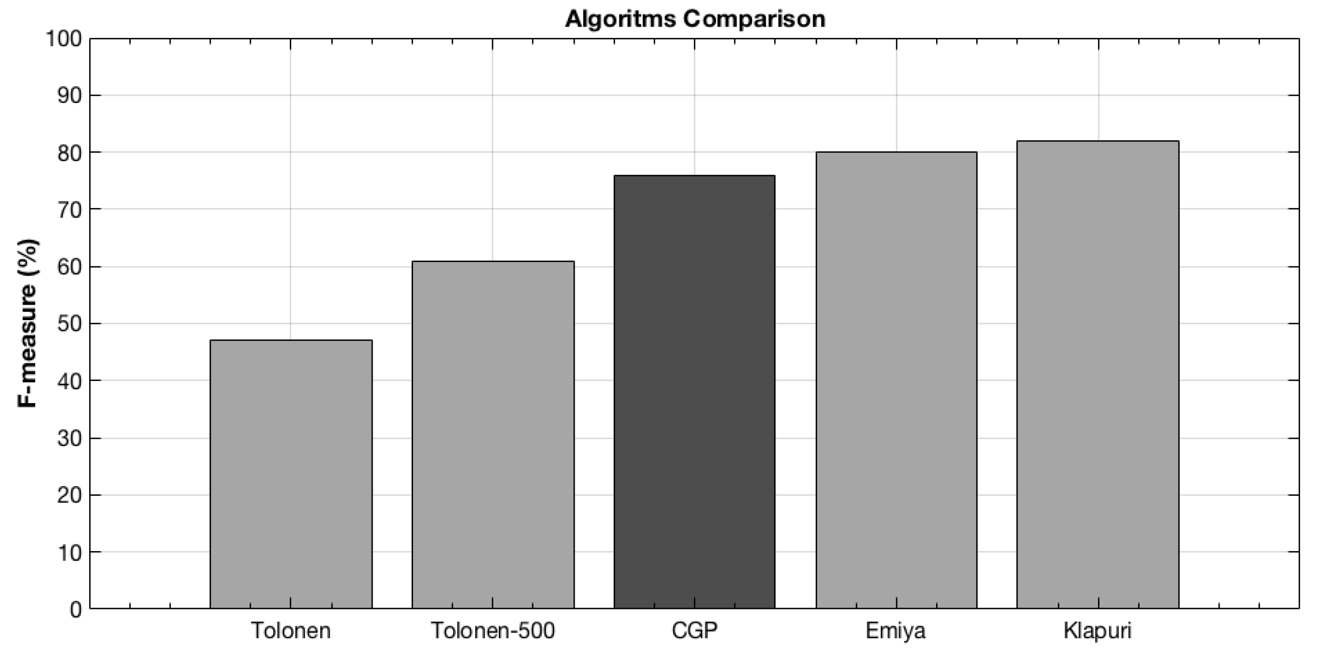
- The accuracy results are in line with the state-of-the-art approaches that use other non-evolutionary methodologies.
- It works with different piano models (upright and grand pianos) and with both digital and acoustic pianos.
- It does not depend on harmony rules, western music rules, or chords construction rules, which was typically the case for previous approaches.
- It uses improved onset detection.
- It provides white-box analyses, which allow other researchers to study the generated models and to use them as an optimization baseline.
- It achieves real-time computing performance.
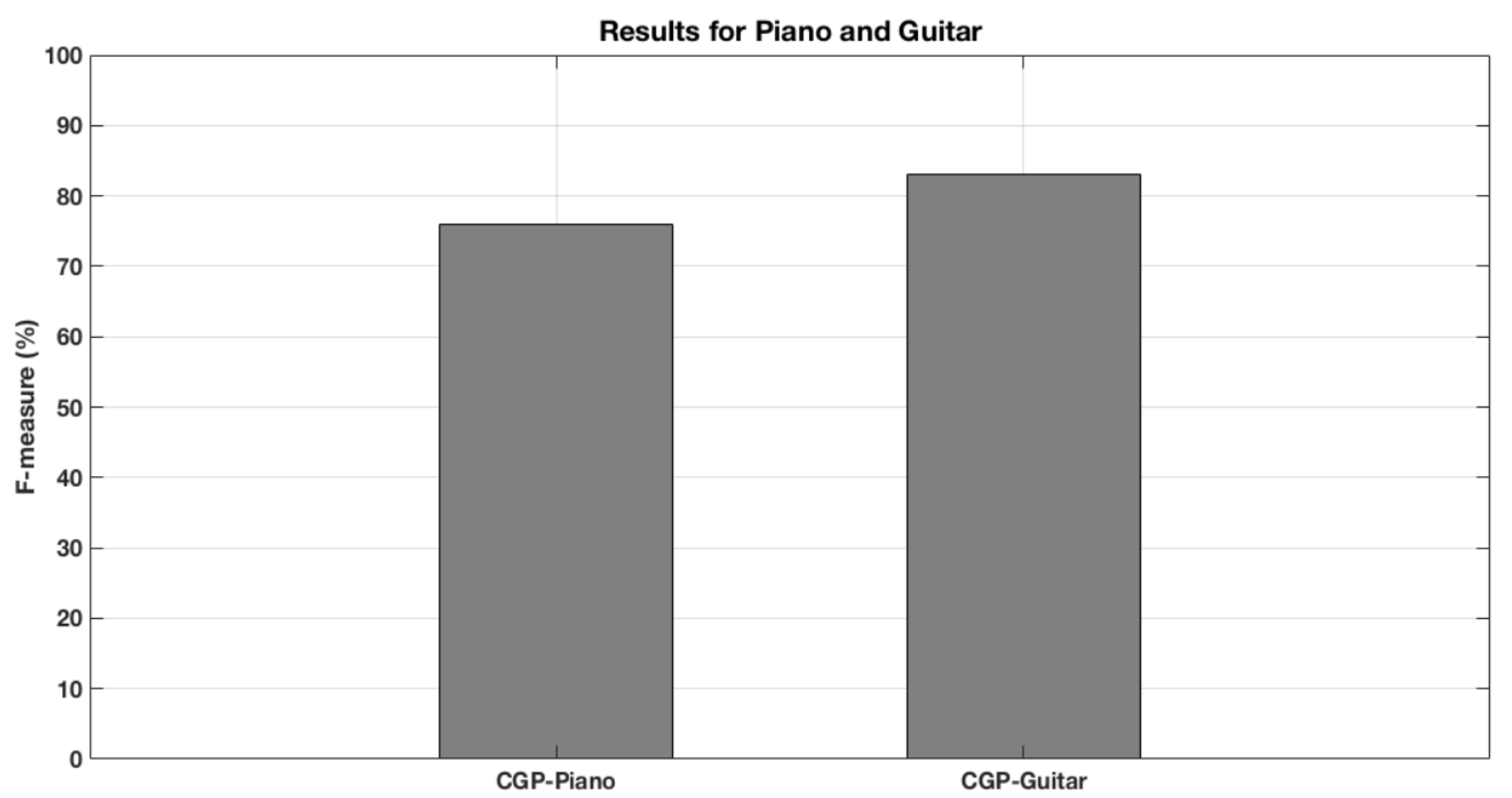
- The technique allows us to perform MPE for other instruments besides piano.
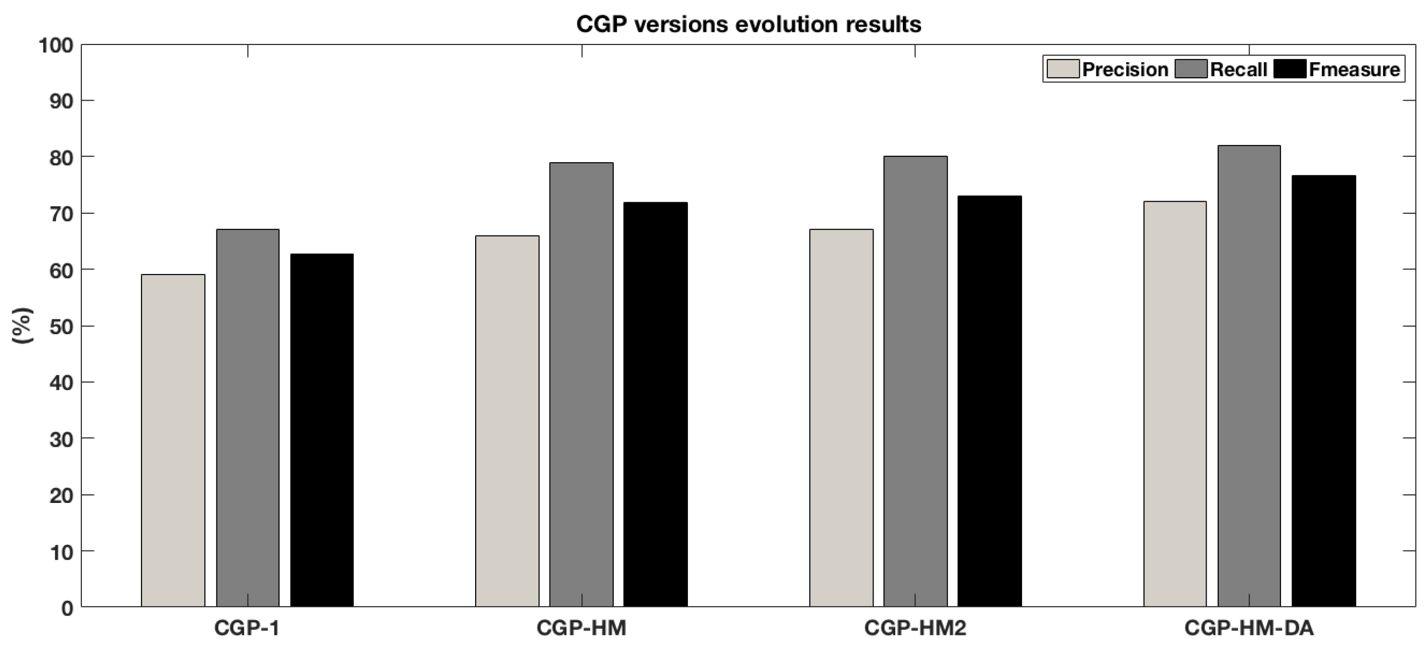
- The significant accuracy results improved compared to our previous approach.
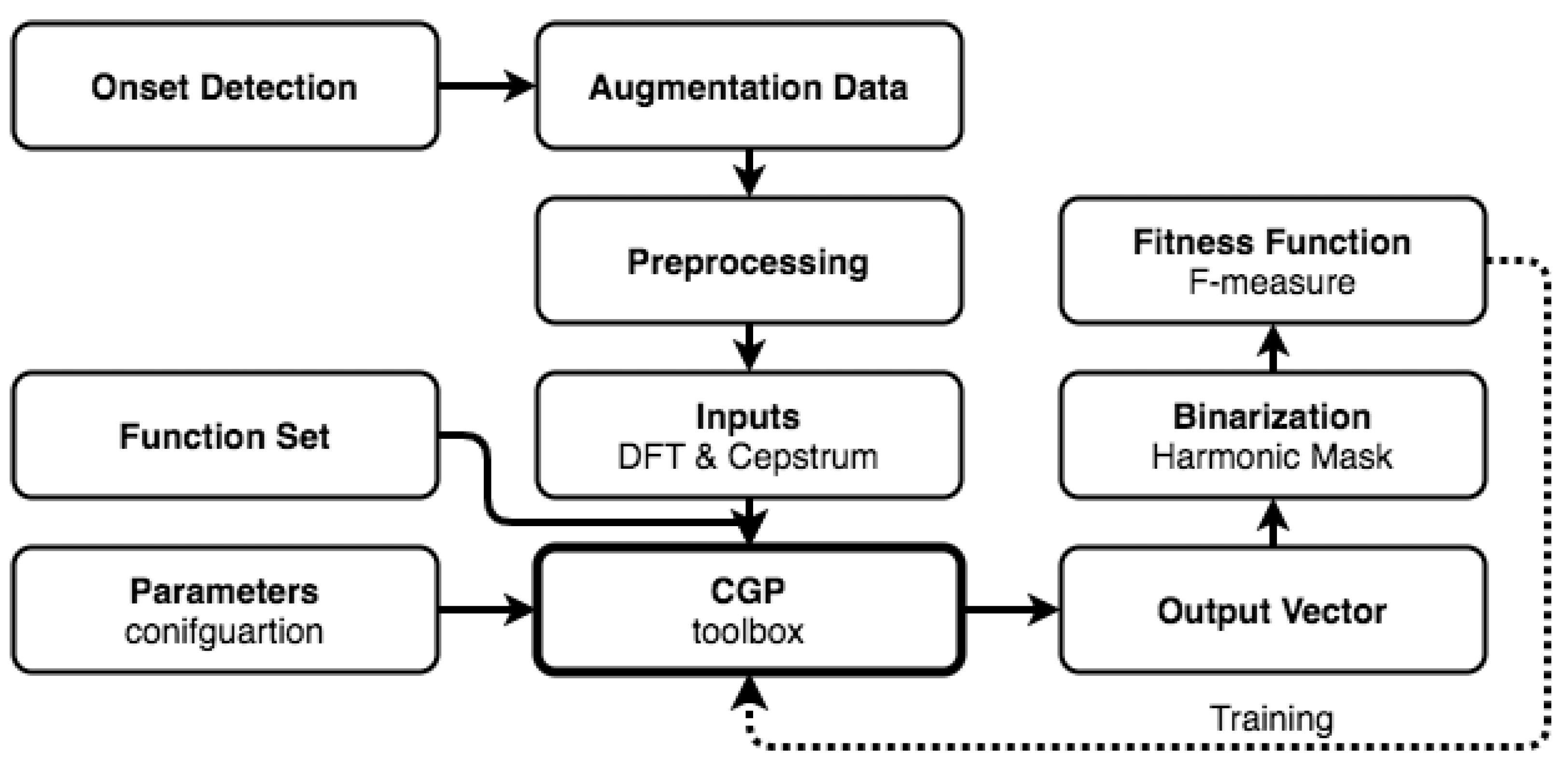
2. System Overview
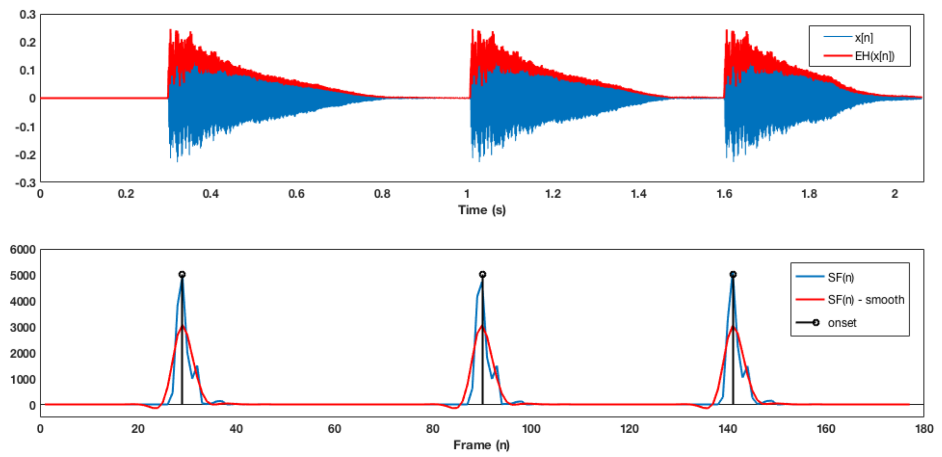
3. Onset Detection
4. Cartessian Genetic Programming
| Algorithm 1 General CGP algorithm. |
|
5. Proposed CGP System
5.1. Training
5.2. Data Augmentation
5.3. Preprocessing
5.4. Inputs
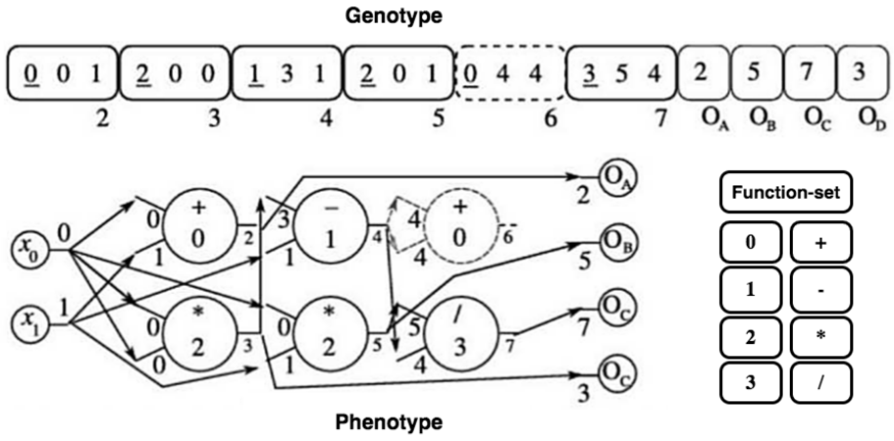
5.5. Individual Encoding
5.6. Mutation
5.7. Evolutionary Strategy
| Algorithm 2 Algorithm . |
|
5.8. Binarization
5.9. Fitness Evaluation
6. Experiments and Results
6.1. Validating the Proposed Methodology
6.2. Classifier Training
6.3. Testing
6.4. White-Box Optimization
6.5. Comparing to Other Approaches
6.6. Reaching for the Piano and Beyond
6.7. Discussion
7. Conclusions and Future Work
Author Contributions
Funding
Institutional Review Board Statement
Informed Consent Statement
Data Availability Statement
Acknowledgments
Conflicts of Interest
Abbreviations
| AMT | Automatic Music Transcription |
| MIR | Music Information Retrieval |
| MIDI | Musical Instrument Digital Interface |
| CGP | Cartegian Genetic Programming |
| MPE | Multi-Pitch Estimation |
| EA | Evolutionary Algorithm |
| CGP4Matlab | Cartesian Genetic Programming for Matlab |
| DFT | Discrete Fourier Transform |
| IDFT | Inverse Discrete Fourier Transform |
| FFT | Fast Fourier Transform |
| STFT | Short Time Fourier Transform |
| HM | Harmonic Mask |
| DA | Data Augmentation |
Appendix A. Function Set
| Index | Function | Description |
|---|---|---|
| 1 | SPAbs | Absolute value |
| 2 | SPBPGaussFilter | Band-pass Gaussian filter |
| 3 | SPCceps | Cepstrum transform |
| 4 | SPConvolution | Convolution |
| 5 | SPCos | Cosine |
| 6 | SPDivide | Point-to-point Division |
| 7 | SPEnvelopeHilbert | Hilbert envelope |
| 8 | SPFFT | Absolute value of the DFT |
| 9 | SPGaussfilter | Gaussian filter |
| 10 | SPHighPassFilter | High-pass filter |
| 11 | SPIFFT | Absolute value of inverst DFT |
| 12 | SPLog | Natural logarithm |
| 13 | SPLog10 | Common logarithm |
| 14 | SPLowPassFilter | Low-pass filter |
| 15 | SPMedFilter | Median filter |
| 16 | SPMod | Remainder after division |
| 17 | SPMulConst | Multiplication by constant |
| 18 | SPNormalizeMax | Normalization maximum |
| 19 | SPNormalizeSum | Normalization sum |
| 20 | SPPeaks | Find peaks |
| 21 | SPPowe | Power |
| 22 | SPSin | Sine |
| 23 | SPSubtract | Subtraction |
| 24 | SPSum | Sum |
| 25 | SPSumConst | Sum with a constant |
| 26 | SPThreshold | Tresholding |
| 27 | SPTimes | Multiplication |
References
- Casey, M.A.; Veltkamp, R.; Goto, M.; Leman, M.; Rhodes, C.; Slaney, M. Content-based music information retrieval: Current directions and future challenges. Proc. IEEE 2008, 96, 668–696. [Google Scholar] [CrossRef]
- Shields, V. Separation of Additive Speech Signals by Digital Comb Filtering. Master’s Thesis, Department of Electrical Engineering and Computer Science, MIT, Cambridge, MA, USA, 1970. [Google Scholar]
- Moorer, J.A. On the transcription of musical sound by computer. Comput. Music J. 1977, 1, 32–38. [Google Scholar]
- Piszczalski, M.; Galler, B.A. Automatic music transcription. Comput. Music J. 1977, 1, 24–31. [Google Scholar]
- Emiya, V. Transcription Automatique de la Musique de Piano. Ph.D. Thesis, Télécom ParisTech, Paris, France, 2008. [Google Scholar]
- Olson, H.F. Music, Physics and Engineering; Courier Corporation: Chelmsford, MA, USA, 1967; Volume 1769. [Google Scholar]
- Lee, C.T.; Yang, Y.H.; Chen, H.H. Multipitch estimation of piano music by exemplar-based sparse representation. IEEE Trans. Multimed. 2012, 14, 608–618. [Google Scholar]
- Yeh, C.; Roebel, A.; Rodet, X. Multiple fundamental frequency estimation and polyphony inference of polyphonic music signals. IEEE Trans. Audio Speech Lang. Process. 2009, 18, 1116–1126. [Google Scholar]
- Goldberg, D.E.; Holland, J.H. Genetic Algorithms and Machine Learning. Kluwer Academic Publishers-Plenum Publishers; Kluwer Academic Publishers: Alphen aan den Rijn, The Netherlands, 1988. [Google Scholar]
- Miller, J.F.; Harding, S.L. Cartesian genetic programming. In Proceedings of the 10th Annual Conference Companion on Genetic and Evolutionary Computation, Atlanta, GA, USA, 12–16 July 2008; pp. 2701–2726. [Google Scholar]
- Harding, S.; Leitner, J.; Schmidhuber, J. Cartesian Genetic Programming for Image Processing. In Genetic Programming Theory and Practice X; Springer: New York, NY, USA, 2013; pp. 31–44. [Google Scholar]
- Benetos, E.; Dixon, S.; Giannoulis, D.; Kirchhoff, H.; Klapuri, A. Automatic music transcription: Challenges and future directions. J. Intell. Inf. Syst. 2013, 41, 407–434. [Google Scholar] [CrossRef]
- Wang, D.; Brown, G.J. Computational Auditory Scene Analysis: Principles, Algorithms, and Applications; Wiley-IEEE Press: Hoboken, NJ, USA, 2006. [Google Scholar]
- Christensen, M.G.; Jakobsson, A. Multi-pitch estimation. Synth. Lect. Speech Audio Process. 2009, 5, 1–160. [Google Scholar] [CrossRef]
- Klapuri, A.P. Multiple fundamental frequency estimation based on harmonicity and spectral smoothness. IEEE Trans. Speech Audio Process. 2003, 11, 804–816. [Google Scholar] [CrossRef]
- Bello, J.P.; Daudet, L.; Sandler, M.B. Automatic piano transcription using frequency and time-domain information. IEEE Trans. Audio Speech Lang. Process. 2006, 14, 2242–2251. [Google Scholar] [CrossRef]
- Saito, S.; Kameoka, H.; Takahashi, K.; Nishimoto, T.; Sagayama, S. Specmurt analysis of polyphonic music signals. IEEE Trans. Audio Speech Lang. Process. 2008, 16, 639–650. [Google Scholar] [CrossRef]
- Dressler, K. Pitch estimation by the pair-wise evaluation of spectral peaks. In Proceedings of the 42nd International Conference: Semantic Audio, Ilmenau, Germany, 22–24 July 2011. [Google Scholar]
- Indefrey, H.; Hess, W.; Seeser, G. Design and evaluation of double-transform pitch determination algorithms with nonlinear distortion in the frequency domain-preliminary results. In Proceedings of the ICASSP ’85. IEEE International Conference on Acoustics, Speech, and Signal Processing, Tampa, FL, USA, 26–29 April 1985; Volume 10, pp. 415–418. [Google Scholar]
- Tolonen, T.; Karjalainen, M. A computationally efficient multipitch analysis model. IEEE Trans. Speech Audio Process. 2000, 8, 708–716. [Google Scholar] [CrossRef]
- Kraft, S.; Zölzer, U. Polyphonic Pitch Detection by Iterative Analysis of the Autocorrelation Function. In Proceedings of the 17th Int. Conference on Digital Audio Effects (DAFx-14), Erlangen, Germany, 1–5 September 2014; pp. 271–278. [Google Scholar]
- Klapuri, A. Multipitch analysis of polyphonic music and speech signals using an auditory model. IEEE Trans. Audio Speech Lang. Process. 2008, 16, 255–266. [Google Scholar] [CrossRef]
- Zhang, W.; Chen, Z.; Yin, F. Multi-Pitch Estimation of Polyphonic Music Based on Pseudo Two-Dimensional Spectrum. IEEE/ACM Trans. Audio Speech Lang. Process. 2020, 28, 2095–2108. [Google Scholar] [CrossRef]
- Goto, M. A predominant-F0 estimation method for polyphonic musical audio signals. In Proceedings of the 18th International Congress on Acoustics, Kyoto, Japan, 4–9 April 2004; pp. 1085–1088. [Google Scholar]
- Cemgil, A.T.; Kappen, H.J.; Barber, D. A generative model for music transcription. IEEE Trans. Audio Speech Lang. Process. 2006, 14, 679–694. [Google Scholar] [CrossRef]
- Kameoka, H.; Nishimoto, T.; Sagayama, S. A multipitch analyzer based on harmonic temporal structured clustering. IEEE Trans. Audio Speech Lang. Process. 2007, 15, 982–994. [Google Scholar] [CrossRef]
- Emiya, V.; Badeau, R.; David, B. Multipitch estimation of piano sounds using a new probabilistic spectral smoothness principle. IEEE Trans. Audio Speech Lang. Process. 2009, 18, 1643–1654. [Google Scholar] [CrossRef]
- Duan, Z.; Pardo, B.; Zhang, C. Multiple fundamental frequency estimation by modeling spectral peaks and non-peak regions. IEEE Trans. Audio Speech Lang. Process. 2010, 18, 2121–2133. [Google Scholar] [CrossRef]
- Peeling, P.H.; Godsill, S.J. Multiple pitch estimation using non-homogeneous Poisson processes. IEEE J. Sel. Top. Signal Process. 2011, 5, 1133–1143. [Google Scholar] [CrossRef]
- Koretz, A.; Tabrikian, J. Maximum a posteriori probability multiple-pitch tracking using the harmonic model. IEEE Trans. Audio Speech Lang. Process. 2011, 19, 2210–2221. [Google Scholar] [CrossRef]
- Yoshii, K.; Goto, M. A nonparametric Bayesian multipitch analyzer based on infinite latent harmonic allocation. IEEE Trans. Audio Speech Lang. Process. 2011, 20, 717–730. [Google Scholar] [CrossRef]
- Vincent, E.; Bertin, N.; Badeau, R. Adaptive harmonic spectral decomposition for multiple pitch estimation. IEEE Trans. Audio Speech Lang. Process. 2009, 18, 528–537. [Google Scholar] [CrossRef]
- Benetos, E.; Dixon, S. A shift-invariant latent variable model for automatic music transcription. Comput. Music J. 2012, 36, 81–94. [Google Scholar] [CrossRef]
- Benetos, E.; Cherla, S.; Weyde, T. An Efficient Shift-Invariant Model for Polyphonic Music Transcription. In Proceedings of the MML 2013: 6th International Workshop on Machine Learning and Music, ECML/PKDD, Prague, Czech Republic, 23 September 2013. [Google Scholar]
- O’Hanlon, K.; Nagano, H.; Plumbley, M.D. Structured sparsity for automatic music transcription. In Proceedings of the 2012 IEEE International Conference on Acoustics, Speech and Signal Processing (ICASSP), Kyoto, Japan, 25–30 March 2012; pp. 441–444. [Google Scholar]
- Keriven, N.; O’Hanlon, K.; Plumbley, M.D. Structured sparsity using backwards elimination for automatic music transcription. In Proceedings of the 2013 IEEE International Workshop on Machine Learning for Signal Processing (MLSP), Southampton, UK, 22–25 September 2013; pp. 1–6. [Google Scholar]
- Fuentes, B.; Badeau, R.; Richard, G. Harmonic adaptive latent component analysis of audio and application to music transcription. IEEE Trans. Audio Speech Lang. Process. 2013, 21, 1854–1866. [Google Scholar] [CrossRef]
- Marolt, M. A connectionist approach to automatic transcription of polyphonic piano music. IEEE Trans. Multimed. 2004, 6, 439–449. [Google Scholar] [CrossRef]
- Sigtia, S.; Benetos, E.; Dixon, S. An end-to-end neural network for polyphonic piano music transcription. IEEE/ACM Trans. Audio Speech Lang. Process. 2016, 24, 927–939. [Google Scholar] [CrossRef]
- Böck, S.; Schedl, M. Polyphonic piano note transcription with recurrent neural networks. In Proceedings of the 2012 IEEE International Conference on Acoustics, Speech and Signal Processing (ICASSP), Kyoto, Japan, 25–30 March 2012; pp. 121–124. [Google Scholar]
- Garcia, G. A Genetic Search Technique for Polyphonic Pitch Detection; ICMC: Geneva, Switzerland, 2001. [Google Scholar]
- Lu, D. Automatic Music Transcription Using Genetic Algorithms and Electronic Synthesis. Bachelor’s Thesis, University of Rochester, Rochester, NY, USA, 2006. [Google Scholar]
- MIDI Manufacturers Association. The Complete MIDI 1.0 Detailed Specification; The MIDI Manufacturers Association: Los Angeles, CA, USA, 1996. [Google Scholar]
- Reis, G.; Fonseca, N.; Ferndandez, F. Genetic algorithm approach to polyphonic music transcription. In Proceedings of the 2007 IEEE International Symposium on Intelligent Signal Processing, Alcala de Henares, Spain, 3–5 October 2007; pp. 1–6. [Google Scholar]
- Reis, G.; De Vega, F.F.; Ferreira, A. Automatic transcription of polyphonic piano music using genetic algorithms, adaptive spectral envelope modeling, and dynamic noise level estimation. IEEE Trans. Audio Speech Lang. Process. 2012, 20, 2313–2328. [Google Scholar] [CrossRef]
- Inácio, T.; Miragaia, R.; Reis, G.; Grilo, C.; Fernandéz, F. Cartesian genetic programming applied to pitch estimation of piano notes. In Proceedings of the 2016 IEEE Symposium Series on Computational Intelligence (SSCI), Athens, Greece, 6–9 December 2016; pp. 1–7. [Google Scholar]
- Miller, J.F.; Thomson, P. Cartesian genetic programming. In Genetic Programming; Springer: Berlin/Heidelberg, Germany, 2000; pp. 121–132. [Google Scholar]
- Miragaia, R.; Reis, G.; Fernandéz, F.; Inácio, T.; Grilo, C. CGP4Matlab-A Cartesian Genetic Programming MATLAB Toolbox for Audio and Image Processing. In International Conference on the Applications of Evolutionary Computation; Springer: Berlin/Heidelberg, Germany, 2018; pp. 455–471. [Google Scholar]
- Miragaia, R.; Reis, G.; de Vega, F.F.; Chávez, F. Multi Pitch Estimation of Piano Music using Cartesian Genetic Programming with Spectral Harmonic Mask. In Proceedings of the 2020 IEEE Symposium Series on Computational Intelligence (SSCI), Canberra, Australia, 1–4 December 2020; pp. 1800–1807. [Google Scholar]
- Martins, L.G. A Computational Framework for Sound Segregation Music Signals. Ph.D. Thesis, University of Porto, Porto, Portugal, 2008. [Google Scholar]
- Rao, K.S.; Prasanna, S.R.M.; Yegnanarayana, B. Determination of Instants of Significant Excitation in Speech Using Hilbert Envelope and Group Delay Function. IEEE Signal Process. Lett. 2007, 14, 762–765. [Google Scholar] [CrossRef]
- Koza, J.R. Genetic Programming: On the Programming of Computers by Means of Natural Selection; MIT Press: Cambridge, MA, USA, 1992; Volume 1. [Google Scholar]
- Koza, J.R. Genetic Programming II: Automatic Discovery of Reusable Subprograms; MIT Press: Cambridge, MA, USA, 1994. [Google Scholar]
- Miller, J.F. Gecco 2013 tutorial: Cartesian genetic programming. In Proceedings of the 15th Annual Conference Companion on Genetic and Evolutionary Computation, Amsterdam, The Netherlands, 6–10 July 2013; pp. 715–740. [Google Scholar]
- Shorten, C.; Khoshgoftaar, T.M. A survey on image data augmentation for deep learning. J. Big Data 2019, 6, 60. [Google Scholar] [CrossRef]
- Emiya, V.; Bertin, N.; David, B.; Badeau, R. Maps-A Piano Database for Multipitch Estimation and Automatic Transcription of Music. Research Report. 2010. Available online: https://hal.inria.fr/inria-00544155 (accessed on 21 March 2021).
- Noll, A.M.; Schroeder, M.R. Real Time Cepstrum Analyzer. U.S. Patent 3,566,035, 23 February 1971. [Google Scholar]
- Hansen, N.; Arnold, D.V.; Auger, A. Evolution Strategies. In Springer Handbook of Computational Intelligence; Kacprzyk, J., Pedrycz, W., Eds.; Springer: Berlin/Heidelberg, Germany, 2015; pp. 871–898. [Google Scholar] [CrossRef]
- Goldman, B.W.; Punch, W.F. Analysis of cartesian genetic programming’s evolutionary mechanisms. IEEE Trans. Evol. Comput. 2015, 19, 359–373. [Google Scholar] [CrossRef]
- Miragaia, R.; Reis, G.; de Vega, F.F.; Chávez, F. Evolving a Multi-Classifier System with Cartesian Genetic Programming for Multi-Pitch Estimation of Polyphonic Piano Music. In Proceedings of the 36th ACM/SIGAPP Symposium Om Applied Computing, Gwangju, Korea, 22–26 March 2021. [Google Scholar]
- Kehling, C.; Abeßer, J.; Dittmar, C.; Schuller, G. Automatic Tablature Transcription of Electric Guitar Recordings by Estimation of Score-and Instrument-Related Parameters; DAFx: Erlangen, Germany, 2014; pp. 219–226. [Google Scholar]
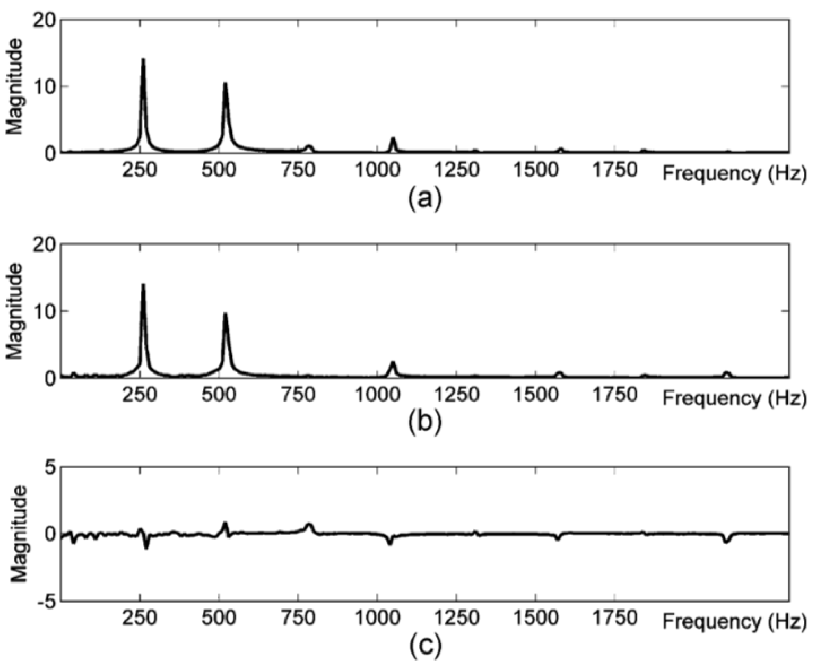



| Parameter | Value |
|---|---|
| K-folds | 5 |
| Data Augmentation | 3 |
| Positive Test Cases | 250 |
| Negative Test Cases | 250 |
| Frame Size | 4096 |
| Fitness Initial Threshold | 1.5 |
| Outputs | 1 |
| Rows | 1 |
| Columns | 100 |
| Levels Back | 100 |
| (E.S. 1 + λ) | 4 |
| Mutation Probability | 5% |
| Threshold Mutation Probability | 6% |
| Harmonic Mask | 2 |
| Runs | 10 |
| Generations | 10,000 |
| Algorithm | Real-Time | Other Instruments | White Box | Piano FM (%) | Guitar FM (%) |
|---|---|---|---|---|---|
| Tolonem | √ | x | x | 47% | - |
| Tolonen-500 | √ | x | x | 61% | - |
| CGP | √ | √ | √ | 76% | 83% |
| Emiya | x | √ | x | 80% | - |
| Klapuri | x | √ | x | 82% | - |
Publisher’s Note: MDPI stays neutral with regard to jurisdictional claims in published maps and institutional affiliations. |
© 2021 by the authors. Licensee MDPI, Basel, Switzerland. This article is an open access article distributed under the terms and conditions of the Creative Commons Attribution (CC BY) license (http://creativecommons.org/licenses/by/4.0/).
Share and Cite
Miragaia, R.; Fernández, F.; Reis, G.; Inácio, T. Evolving a Multi-Classifier System for Multi-Pitch Estimation of Piano Music and Beyond: An Application of Cartesian Genetic Programming. Appl. Sci. 2021, 11, 2902. https://doi.org/10.3390/app11072902
Miragaia R, Fernández F, Reis G, Inácio T. Evolving a Multi-Classifier System for Multi-Pitch Estimation of Piano Music and Beyond: An Application of Cartesian Genetic Programming. Applied Sciences. 2021; 11(7):2902. https://doi.org/10.3390/app11072902
Chicago/Turabian StyleMiragaia, Rolando, Francisco Fernández, Gustavo Reis, and Tiago Inácio. 2021. "Evolving a Multi-Classifier System for Multi-Pitch Estimation of Piano Music and Beyond: An Application of Cartesian Genetic Programming" Applied Sciences 11, no. 7: 2902. https://doi.org/10.3390/app11072902
APA StyleMiragaia, R., Fernández, F., Reis, G., & Inácio, T. (2021). Evolving a Multi-Classifier System for Multi-Pitch Estimation of Piano Music and Beyond: An Application of Cartesian Genetic Programming. Applied Sciences, 11(7), 2902. https://doi.org/10.3390/app11072902


