1. Introduction
High lift devices such as leading edge (LE) slats and trailing edge (TE) flaps have been effectively employed for many years to increase the lifting performance of aircraft wings during take-off and landing. Conventional slats and flaps used by the aviation industry today consist of movable, split, or hinged mechanical sections with or without slotted surfaces. A modern alternative to the abovementioned articulated multi-element high lift devices is based on shape morphing concept, like the droop nose LE and the morphed TE. Morphed wings can attain similar aerodynamic performance characteristics to those of conventional high lift devices by tailoring the shape (both mean-line curvature and local thickness distribution) of the wing airfoil sections through the deployment of smart material elements at the LE and TE regions.
Smart materials have the property of altering their shape when variable external conditions are imposed (e.g., Shape Memory Alloys—SMAs—deform through heating and cooling). In this way, varying LE and TE shapes can be achieved using lightweight distributed actuators, acting locally on the smart material elements. By following the above approach vulnerable complex and heavy mechanical parts can be avoided. Additionally, a seamless surface geometry is attained eliminating large gaps or slots of multi-element devices, which constitute the main source of high frequency noise emission during take-off and landing. A typical example of morphing control is the droop nose airfoil, which compared to the traditional slat, exhibits lower drag levels (better aerodynamic performance) and better stall characteristics. However, the sole use of the droop nose wing cannot ensure as high levels of the maximum lift coefficient (CL,max) and the stall angle of attack (AoA) as those obtained by two- or three-elements slats.
Research on high-lift devices has been carried out for several decades. Gillis and McKee [
1] studied the behavior of NACA23012 airfoil in a wind tunnel, using a Maxwell LE slat and a slotted and a split flap. Their target was to determine the optimum slot gap and investigate the aerodynamic characteristics of the airfoil for several deflection angles of both types of flap. The optimum slot gap of 0.0175% of the chord increased the C
L,max and stall AoA considerably. The effectiveness of the slat, however, dropped off with increasing flap deflection. Axelson and Stevens [
2] investigated the aerodynamic performance of NACA 64A010 with slat in a wide range of Mach and Reynolds numbers. Two families of slats were employed, one with the LE slat extended forward along the airfoil chord line, and the other with the slat extended forward and displaced below the chord line. At lower Mach number tests, the highest maximum lift values were measured with the slat nose displaced below the wing chord line. However, at Mach numbers higher than 0.7, adverse effects such as a large increase in drag and in the zero lift angle of attack resulted with the slat nose below the airfoil chord line.
Until the beginning of 1990, substantial research effort focused on the determination of the optimum position for the different flap and slat types. Investigations included many different experiments, using either flap or slat or their combination. Moreover, the effect of high lift devices at different flight stages, speeds, and altitudes was analyzed. Rudolph [
3] made an extensive review of the available high-lift devices, their functions, and design criteria. He appraised the high-lift systems of the commercial aircrafts of his time, presented personal study results, and developed a weight and cost model. He concluded that there was still margin for improvement in terms of weight, cost, and aerodynamic performance, pointing to the direction of reduced complexity, increased reliability, and lower weight, while maintaining or improving aerodynamic performance. Monner et al. [
4] developed the concept of a “smart” slat without slot as an alternative to the conventional droop nose utilized on A380 aircraft. The main emphasis of the new device was on realizing a structure/system solution for a smooth leading surface, which can be deflected into a typical high lift application. The approach employed flexible panels on the upper and lower surface of the device in order to provide a continuous curvature distribution over the device chord. The simulation results proved the feasibility of the device and pointed out the need for materials with improved strength for morphing applications.
Burnazzi and Radespiel [
5] evaluated the potential of gapless droop nose devices designed for improving the aerodynamics of airfoils with active high lift. Flexible droop nose configurations were obtained by smoothly morphing the baseline LE shape. Increasing the stall angle of attack and reducing the power required by the active high-lift system were the main objectives. The most promising droop nose configurations were compared with a conventional slat device as well as with the clean LE. Another droop nose investigation was carried out by Wang et al. [
6], who performed CFD simulations to study the aerodynamic characteristics of the two-element airfoil with droop nose, based on the British NHLP 2-D L1T2 three-element airfoil with slat. Numerical results showed that the three-element airfoil with slat produced a higher C
L at the tail-scrape angle, as well as a much higher C
L,max than the two-element airfoil with droop nose. On the other hand, the two-element airfoil with droop nose had a much higher critical aerodynamic factor at the second-segment climb stage (lift to drag ratio when C
L = C
L,max/1.13
2). By deflecting the Fowler flap and the spoiler, the aerodynamic characteristics of the two-element airfoil with droop nose were improved; C
L at the tail-scrape angle surpassed that of the three-element airfoil with slat, maintaining at the same time a higher lift-to-drag ratio. However, the three-element airfoil still exhibited a higher C
L,max due to larger stall AoA. Tian et al. [
7] introduced the flexible variable camber TE flap to improve flight efficiency during take-off, cruise, and landing. A multi-objective optimization with a numerical simulation method indicated that, compared to the traditional flap, C
L was considerably increased during take-off and landing (8% and 1.3% respectively), whilst under cruise state, the lift to drag ratio reached a maximum increment of about 30% over a wide range of C
L. Finally, in their recent research, Magrini and Benini [
8] performed an aerodynamic optimization of a morphing leading edge based on the class/shape transformation technique, incorporating a procedure to keep the arc length of the curve constant in order to limit the axial stress of the deformed shapes. The main benefit of the morphing leading edge was a substantial drag reduction, whereas the lift was less positively affected. A metamodel-assisted optimization loop through the use of an artificial neural network was proven suitable for reducing the computational effort.
In previous investigations, morphing is applied and assessed either on the LE or on the TE region of an airfoil. In the present work, combined morphing of both LE and TE regions is applied and the potential of increasing the CL,max of a typical aircraft airfoil is investigated. The target of the work is twofold: First, the development of a fast methodology capable of delivering the optimum morphed airfoil designs in terms of the CL,max increase and second, the physical understanding of the effect of morphing on the CL,max and the stall AoA through a detailed flow field inspection. As baseline airfoil, the typical in aircraft applications, NACA 64A010, has been selected. Morphed LE and TE shapes are approximated using Bezier curves derived from a number of 11 and 9 control points, locally defined in the vicinity of the LE and TE regions, respectively. The vertical positions of the control points constitute the design variables of a design optimization loop, which is thereafter followed in order to obtain the LE and TE shapes, which provide maximum CL and stall AoA. The procedure of defining the search space of the control points is described in detail and may constitute a guideline for future works on design optimization.
In the optimization process, candidate morphed solutions are requested to satisfy certain geometrical constraints regarding smoothness of the surface curvature, while their aerodynamic performance characteristics (lift and drag polars) are obtained using Foil2w, a fast viscous-inviscid interaction in-house solver [
9]. The objective function of the optimization process is the maximum lift coefficient C
L,max. In order to reduce the computational cost and render the entire process efficient, three different categories of optimization algorithms are tested. Apart from the traditional and most commonly used in design problems, Genetic Algorithm, the alternative of Evolutionary Strategies and the more modern Particle Swarm Optimizer are applied and evaluated. Optimum designs stemming from the design optimization loop are verified through simulations using the in-house Unsteady Reynolds Averaged Navier-Stokes (URANS) solver MaPFLow [
10]. In addition to the verification purpose, CFD aerodynamic simulations (a) provide better understanding and physical insight of the local flow characteristics over the modified portions of the airfoil section, which are directly linked to the resulting distributed and overall aerodynamic loads and (b) estimate the change in the aerodynamic performance (C
L/C
D) using the morphed airfoils. Hence, CFD simulations serve the scope of interpreting the results obtained, but also ensure the overall aerodynamic effectiveness of the design.
The following text is organized as follows: In
Section 2, the optimization procedure along with the solvers employed for the flow simulations are described. The application and the results of the methodology are presented in
Section 3.
Section 4 refers to the verification of the aerodynamic results obtained through the optimization chain for selected morphing designs using the CFD solver. Finally, in the last section, the main conclusions of the work are reported and discussed.
2. Methodology
Three representative stochastic algorithms are integrated into the optimization process, all included in the Inspyred library of Python [
11]: Genetic Algorithm (GA), Evolution Strategies (ES) and Particle Swarm Optimizer (PSO). All of them are members of the Evolutionary Algorithms (EA) [
12,
13] and share a great number of common features. They are population-based performing with best-to-survive criteria. EA algorithms are considered suitable for design optimization of airfoils, therefore they have been selected in the present work instead of other methods, such as deterministic gradient-based algorithms, which may present convergence difficulties during the optimization process. GA [
14] is the most traditional category, especially in the fields of Aerodynamics and Turbomachinery. It resembles the members of population with chromosomes and applies the typical operators of crossover and mutation to evolve to the next generation. ES algorithm [
15] applies the mutation and recombination operators not only on the design variables, but also on endogenous strategic parameters such as the mutation strength. It usually employs encoding of design variables in the field of real and not binary numbers as GA does. PSO algorithm [
16] has been in application for the last two decades. It represents each solution as a particle and the population of solutions is called a swarm of particles. The best positions of each particle and of the swarm are continuously updated and the velocities are adjusted based on the experiences of the particles. The procedure stops when the position of the swarm satisfies the criterion for the objective function.
In the following the optimization problem is outlined. This requires definition of the objective function, the design variables of the problem and the necessary geometric design constraints, which ensure that physically acceptable solutions are obtained, while at the same time prevent unnecessary computations for geometrically inconsistent candidate solutions. In the present analysis, as objective function the maximum lift coefficient (CL,max) of the morphing airfoil shape is chosen, under specific conditions with respect to the freestream, i.e., specific values of Reynolds (Re) and Mach (Ma) numbers. The baseline airfoil (undeformed shape of wing cross section) is chosen as the starting design of the optimization process and its coordinates are normalized with respect to the chord. In order to maximize CL,max, the shape of the baseline airfoil is modified at the LE and TE regions, defined by the intervals (0, 0.25) and (0.8, 1) of the x-coordinate, respectively. The design variables are the y-coordinates of the control points of the Bezier curves used in approximating the airfoil morphing shapes. The control points are only allowed to move vertically. In the present work, the Bezier curves approximation method has been chosen due to its flexibility in representing smooth geometries, such as airfoil deformations, by altering the positions of the control points.
Curvature and slope constraints are imposed to avoid irregularities and discontinuities of the derived geometries and to ensure a smooth connection between deformed and undeformed parts. These constraints are related to:
- (a)
The slope variations of the airfoil geometry. Large changes in the geometry gradients should not be permitted and this is checked by the product of the gradients (first derivatives) of consecutive segments of the discretized geometry. In the case that negative values of this product less than −10−3, are obtained, the current airfoil geometry is rejected.
- (b)
The maximum curvature of the LE geometry, which undergoes the highest deformations. An upper limit is set for the curvature of the upper and lower parts of the deformable LE geometry. The curvature is calculated with respect to the second and the first derivative.
The viscous-inviscid flow solver used for the prediction of C
L and C
D polars of the designed shapes during the optimization procedure is the in-house Foil2w code [
9]. It is a low-cost viscous-inviscid interaction model, formulated on the basis of a standard panel method combined with a vortex blob approximation of the wake, in which the “equivalent inviscid flow (EIF)” velocity
is expressed in the form:
where
is the velocity of the purely potential flow and
is the correction term that needs to be added in order to account for viscous effects. The potential flow part
is simulated on the basis of a standard panel formulation by distributing singularities along the airfoil geometry (piecewise constant sources and constant vorticity), while the wake is represented by free vortex particles, which are convected with the local flow velocity. The modeling of the viscous correction part
is also based on an integral representation (integration over the airfoil
and the wake
):
where
is the normal correction velocity on
and
the normal correction velocity jump on
, while
is the tangential correction velocity on
(note that tangential correction velocity jump in the wake is omitted).
The viscous flow solution (the integral boundary layer quantities, displacement thickness, and momentum thickness) is obtained by solving the unsteady integral boundary layer equations as formulated in steady-state form by Drela and Giles [
17] and re-casted in their unsteady form by Riziotis and Voutsinas [
9]. The viscous-inviscid interaction coupling is achieved through the normal to the wall and the wake shear layer transpiration velocity distribution that represents the mass flow difference between the real viscous flow and the equivalent inviscid flow within the boundary layer, given by:
As seen in Equation (3), in the wake, the transpiration velocity jump is calculated by summing up the mass deficit of the upper and lower side of the wake shear layer. The boundary layer solution is supplemented by a transition prediction model based on the e
N spatial amplification theory [
18]. It is noted that Foil2w has been thoroughly validated against measurements on an airfoil undergoing harmonic pitching motion [
9].
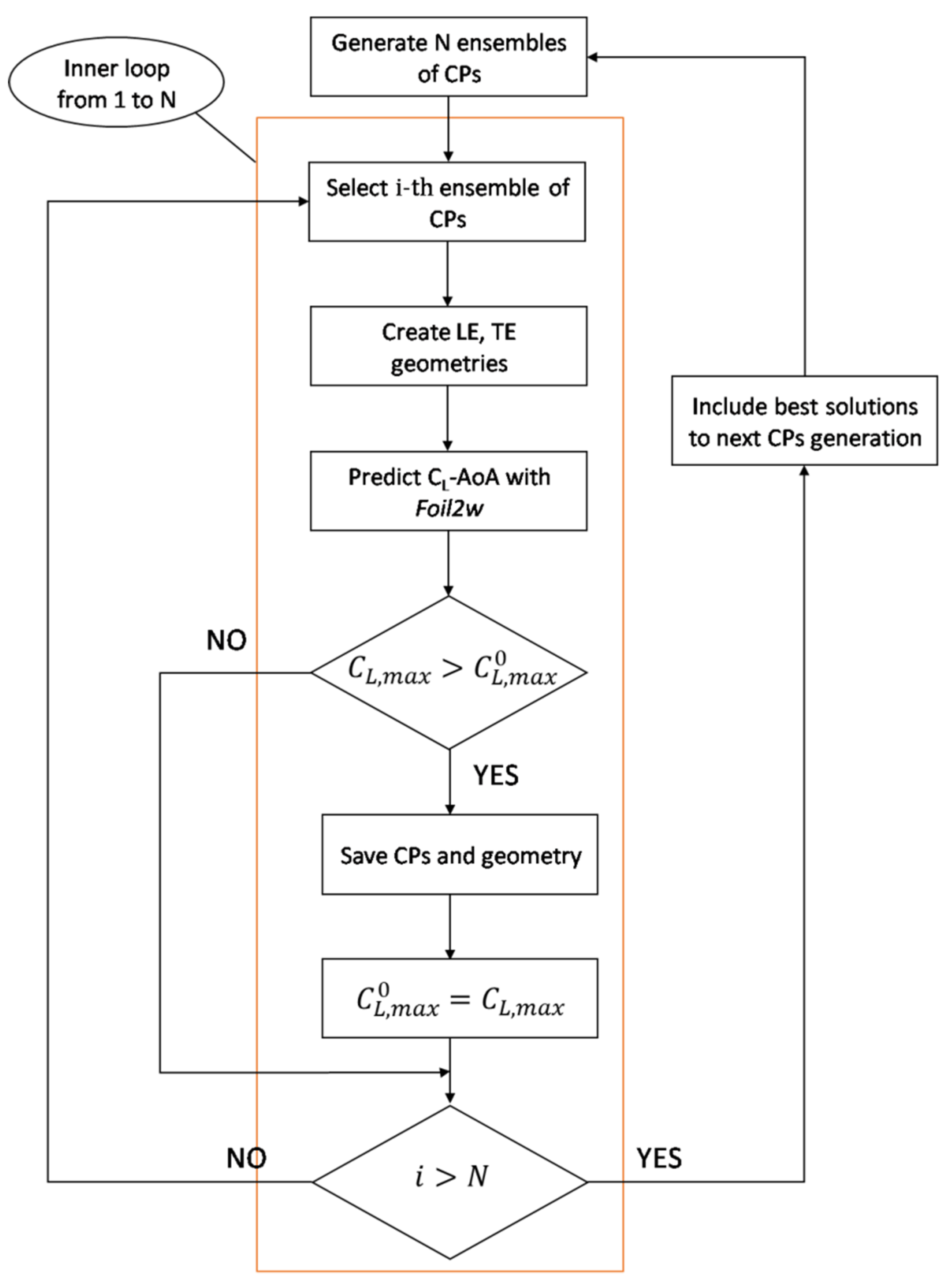
The flow chart of the optimization process is illustrated in
Figure 1. Random combinations (ensembles) of control points are generated and create Bezier curves that approximate the LE and TE regions. They represent an initial population of solutions (geometries). Every single airfoil is evaluated using Foil2w: the polar C
L-AoA is predicted and the maximum lift coefficient value C
L,max is compared to the one of the previous airfoil (starting value of C
L,max is that of the baseline airfoil). If C
L,max increases, geometry and control points (design variables) are saved and a new population (generation) is generated, based on the best solutions of the current set studied.
The final morphing shapes selected through the optimization process are verified through high fidelity CFD simulations. The URANS CFD solver employed for the validation of the Foil2w predictions is the in-house MaPFlow code [
10]. It is a multi-block MPI enabled compressible solver equipped with the Eriksson’s preconditioner [
19] to handle regions of low Mach flow. The discretization scheme for the convective fluxes is cell centered and makes use of the Roe approximate Riemann solver [
20]. In space, the scheme is 2nd-order accurate defined for unstructured grids and applies the Venkatakrishnan’s limiter [
21]. In time, the scheme is 2nd-order accurate and implicit utilizing dual time stepping to facilitate convergence. The solver is equipped with the Spalart-Allmaras (SA) [
22] and the k-ω SST [
23] eddy viscosity turbulence models. Regarding transition, three models have been implemented, the correlation γ-Re
θ model of Menter [
24], the Granville/Schlichting transition method described in [
25], and the e
N model described in [
26]. MaPFlow has been thoroughly validated against experimental data in many steady and unsteady airfoil simulations including simulation of flow control devices such as vortex generators [
27] and TE flaps [
28]. In [
28] both MaPFlow and Foil2w, predictions were validated against measurements in static (steady) and oscillating (unsteady) TE flap cases.
3. Optimization Results
For the optimization process, NACA 64A010 is used, as it is a common airfoil for aircraft applications. The ambient flow conditions employed in the numerical analyses are M = 0.22 and Re = 6 × 10⁶, corresponding to typical take-off and landing conditions of a short to medium range aircraft with flight speed of 75 m/s and a chord length of 1.2 m (close to the tip of the aircraft wing).
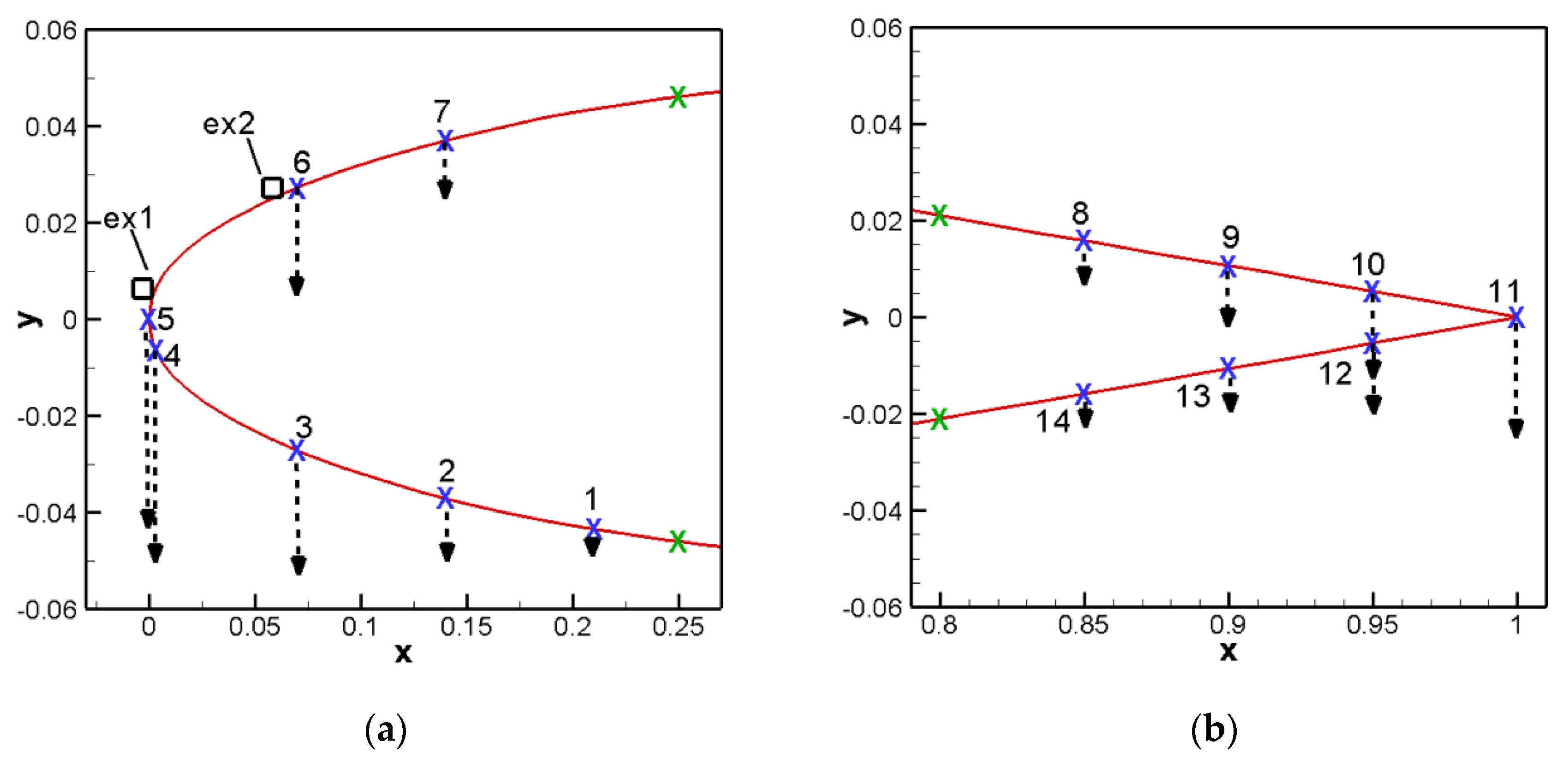
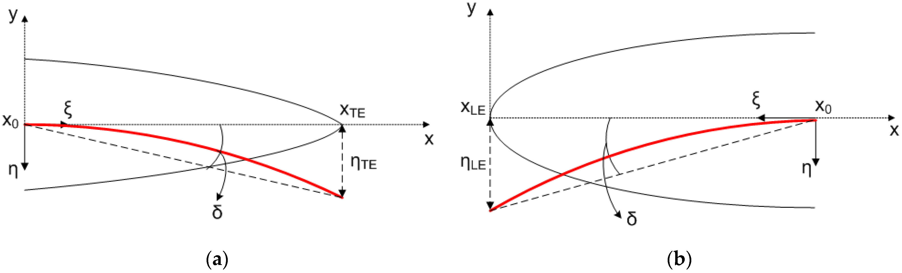
Separate Bezier curves are produced for the TE and the LE regions considering a separate group of control points for each one of them. Both the suction and pressure side geometry, either of the LE or the TE region, are represented by the same curve. The x-coordinates of the control points used in the present analysis are pre-selected as illustrated in
Figure 2 and they are not modified throughout the optimization procedure. A preliminary study is made to determine the optimum number of control points for the LE and TE regions. A total of nine control points is found sufficient for reproducing the sharp TE shape of the airfoil section with reasonable detail. Less points result in significant geometrical irregularities, demanding additional constraints that is not obvious to determine. More points increase the possible combinations and the computational cost of the optimization procedure. Two of the control points are placed at the connections between the undeformed and the morphing parts of the airfoil (one on the upper and another on the lower side respectively) and remain fixed throughout the optimization process. The remaining points are divided between the upper and lower side (three on the upper side, three on the lower side, and one at the TE point) and they are only allowed to move vertically. As shown in
Figure 2b, expected deflections in the TE region will be relatively small and therefore it is sufficient to simply distribute control points at equal distances along the
x-axis (
Figure 2b). The y-coordinates of the seven movable control points constitute the design variables of the optimization loop for the TE morphing shape.
A similar approach is followed for the LE region. Again, two control points remain fixed, connecting the undeformed with the morphing part, and seven control points are distributed on the two sides, three on the upper and four on the lower side, as shown in (
Figure 2a). Again, the y-coordinates of the seven control points constitute the design variables of the optimization loop. However, there are some differences compared to the approach followed at the TE region: First, more control points are needed close to the LE in order to maintain the rounded shape of the LE region. Therefore, the control point 4 of the lower side (CP4) must be located very close to the LE control point (CP5). Furthermore, on the upper side two extra control points ex1, ex2 are added (
Figure 2a). The x,y-coordinates of the ex1 additional control point are derived through linear extrapolation to the x,y-coordinates of CP4 and CP5. The x,y-coordinates of the ex2 additional control point are defined so that the curvature of the lower side (points CP3,CP4,CP5) is similar to that of the upper side (points CP5,ex1,ex2), maintaining thus the roundness of the LE. Since the y-coordinates of the ex1, ex2 points depend on the y-coordinates of the control points 3, 4, 5, they are not considered as independent design variables. Second, an additional control point, CP1, is needed at the lower side, close to the quarter of chord, in order to avoid abrupt gradient changes between the morphing and the undeformed geometries that may cause flow disturbances. An overall number of 11 control points are used for determining the Bezier curve of the LE region (
Figure 2a).
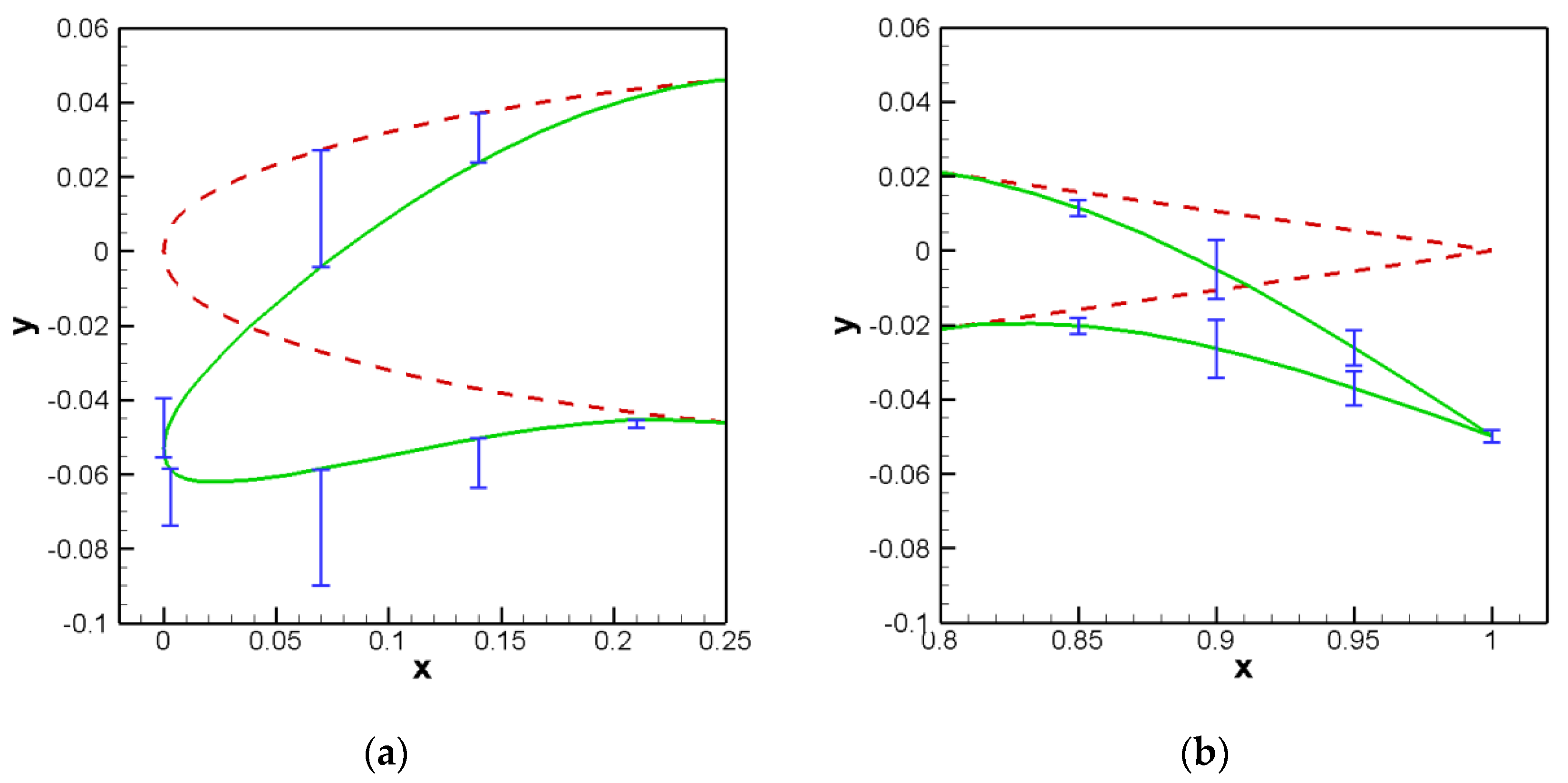
The y-coordinates of the 14 variable control points (7 for the TE and 7 for the LE regions) vary within specific ranges, which constitute an input parameter of the design process. A proper selection of the above ranges ensures that acceptable LE and TE shapes are generated during the optimization loop and that no redundant computational cost is added to the computations. Proper selection consists in choosing the smallest possible intervals through which overlapping of the allowable y-coordinate range of neighboring control points is avoided. In this way the number of non-physical solutions, such as “wavy” geometries is reduced. Even though non-physical solutions may be finally excluded through the geometrical constraints, unnecessary design computations are added when large intervals are considered. An initial estimation of the intervals level is obtained using a reference deformation shape of the original airfoil geometry for given LE and TE deployment angles: The mean airfoil line is deformed through a polynomial relationship with respect to the distance from the LE (or TE) (see
Appendix A), whilst the initial thickness at each x-position is retained. In the present work, the LE and TE deployment angles are chosen as 12° and 14° respectively.
In the TE region, the shape of the reference deformation is used to define the mean value of each control point’s interval. For CPs 8, 9, 13, and 14 (numbering of points is shown in
Figure 2b), the difference between the y-coordinates of the baseline (undeformed) and the deformed airfoil is used as the interval width. For the TE point 11, the interval width is kept small and corresponds to a ±3% deviation with respect to the TE deployment angle of 14°. For points 10 and 12, the interval width is set 1.5 times larger than that of the TE point 11. The selected ranges for the TE control points are depicted in
Figure 3b. In the LE region, higher overall deformations are required in order to substantially affect the overall loading of the airfoil. On the upper side the shape of the reference deformation is used to define the lower bound of each control point’s interval, whilst on the lower side the reference deformation is used to define the upper bound of each control point’s interval. For CPs 1, 2, 3, 6, and 7 (numbering of points is shown in
Figure 2a), the difference between the y-coordinates of the baseline (undeformed) and the deformed airfoil is used as the interval width. For LE points 4 and 5, the interval width corresponds to a 25% deviation with respect to the LE deployment angle of 12°. The selected ranges for the LE control points are depicted in
Figure 3a.
In the following, the three optimization algorithms described in
Section 2 are tested for the case of combined LE and TE morphing. In
Table 1, the C
L,max values obtained by the three algorithms are provided as a function of the number of generations of the optimization process. The optimization setup is the same for all three algorithms, meaning that the same number of initial airfoils are created and the same number of offspring are produced at each generation. In the present work, the default number of offspring is used, defined as 8 times the number of the design variables (8 × 14 = 112). Therefore, the number of total fitness evaluations equals the product of the total generations multiplied by the number of offspring at each generation, plus the initial population. As an example, for the maximum number of generations (17), the number of fitness evaluations is 17 × 112 + 112 = 2016. For the current setup, PSO algorithm outperforms the other two algorithms as it predicts the solution with the maximum C
L,max, while it requires the minimum number of generations (4). ES algorithm requires a significantly larger number of generations (17) to reach about the same C
L,max level (2% lower). On the other hand, the optimum design predicted by the GA algorithm after 17 generations, has a maximum C
L,max value 7% lower than that of the PSO algorithm. Comparing ES against GA, it is observed that the ES algorithm achieves a higher C
L,max value at the expense of computational time, as it requires 17 generations in order to reach that solution. GA reaches a solution with a slightly higher C
L,max (2.5% difference) at a lower number of generations (after only eight generations).
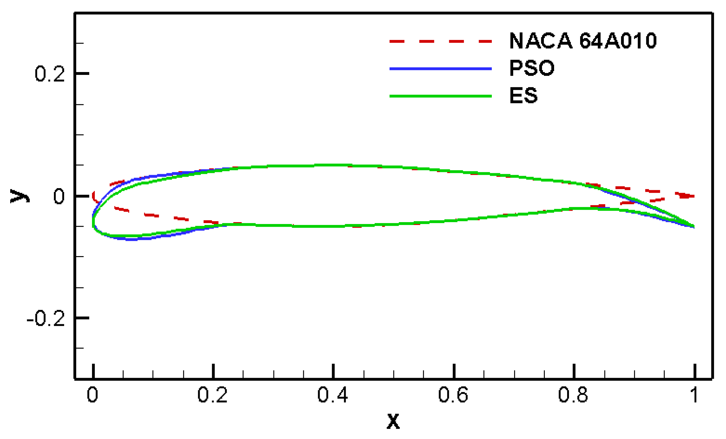
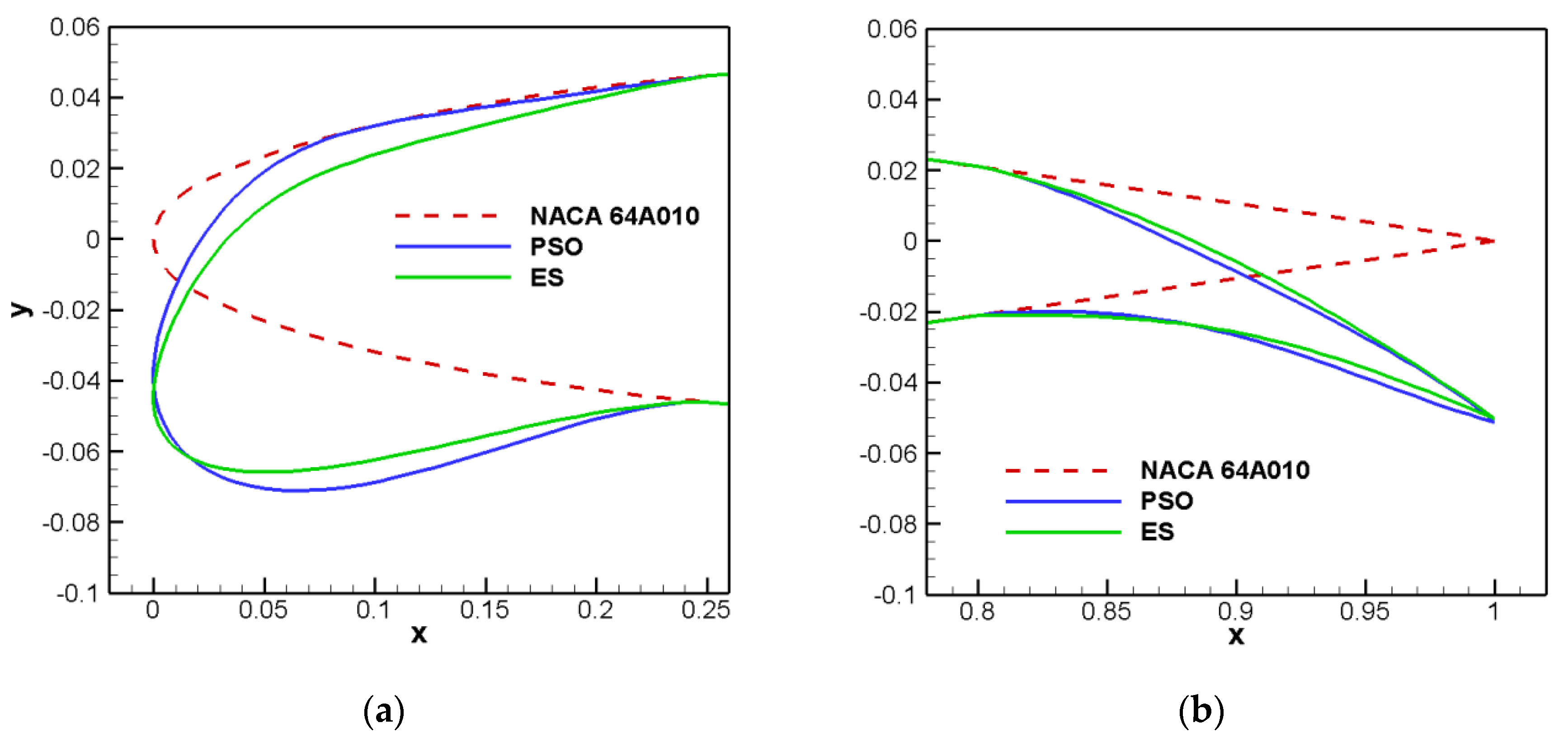
The resulting optimum morphing shapes produced by the three algorithms are then compared in terms of the required airfoil shape deformation in order to reach their maximum C
L,max. Shape deformation is measured in terms of the percentage of increase of the airfoil skin length at the morphing regions with respect to the corresponding lengths of the baseline undeformed airfoil.
Table 2 summarizes these percentages separately at the LE and TE regions as well as for the overall skin length. In general, two shape types of geometries are produced by the three algorithms, the first type with the highest C
L,max (>2.2) presenting larger deformations at the LE region (≈5.7%), and the second type with C
L,max ≈ 2.1 presenting smaller deformations at the LE region (≈4.5%). Similar TE deformations are predicted for both types of morphed designs.The solution of GA after eight generations and the solution of ES after eight generations belong to the first type. The solution of ES after 17 generations and the solution of PSO after 4 generations belong to the 2nd type.
Figure 4 presents one morphed geometry per airfoil type; the PSO first type after four generations and the ES second type after eight generations. In the subsequent analysis, the ES solution is preferred instead of the corresponding GA solution, since it is considered as more representative of the second type (smaller deformation at the LE region). Differences between the two shapes are highlighted in the focus plot of
Figure 5. The second type solution could qualify as preferred design, e.g., in the case of an upper limit on allowable LE deformation, imposed by constraints on material properties (maximum stress level) or actuator limitations.
It is noted that in the current setup, a rather “aggressive” design has been chosen in terms of the permitted deformations. At the LE region, the droop nose part corresponds to the 25% of the chord length, both on the upper and lower sides, whilst at the TE region the deformable flap corresponds to the 20% of the chord length. In some of the previous investigations [
4,
5,
6], more conservative approaches have been adopted to avoid possible discontinuities, especially on the upper side of the droop nose part. The present algorithm can be easily adapted to such approaches by keeping the control points 1 and 7 fixed at the LE part (
Figure 2a), as well as the points 8 and 14 at the TE part (
Figure 2b). In this way, the deformable parts of the LE and TE regions are restricted to 20% and 15%, respectively. Moreover, an even smaller deformation is permitted for the upper side of the droop nose part.
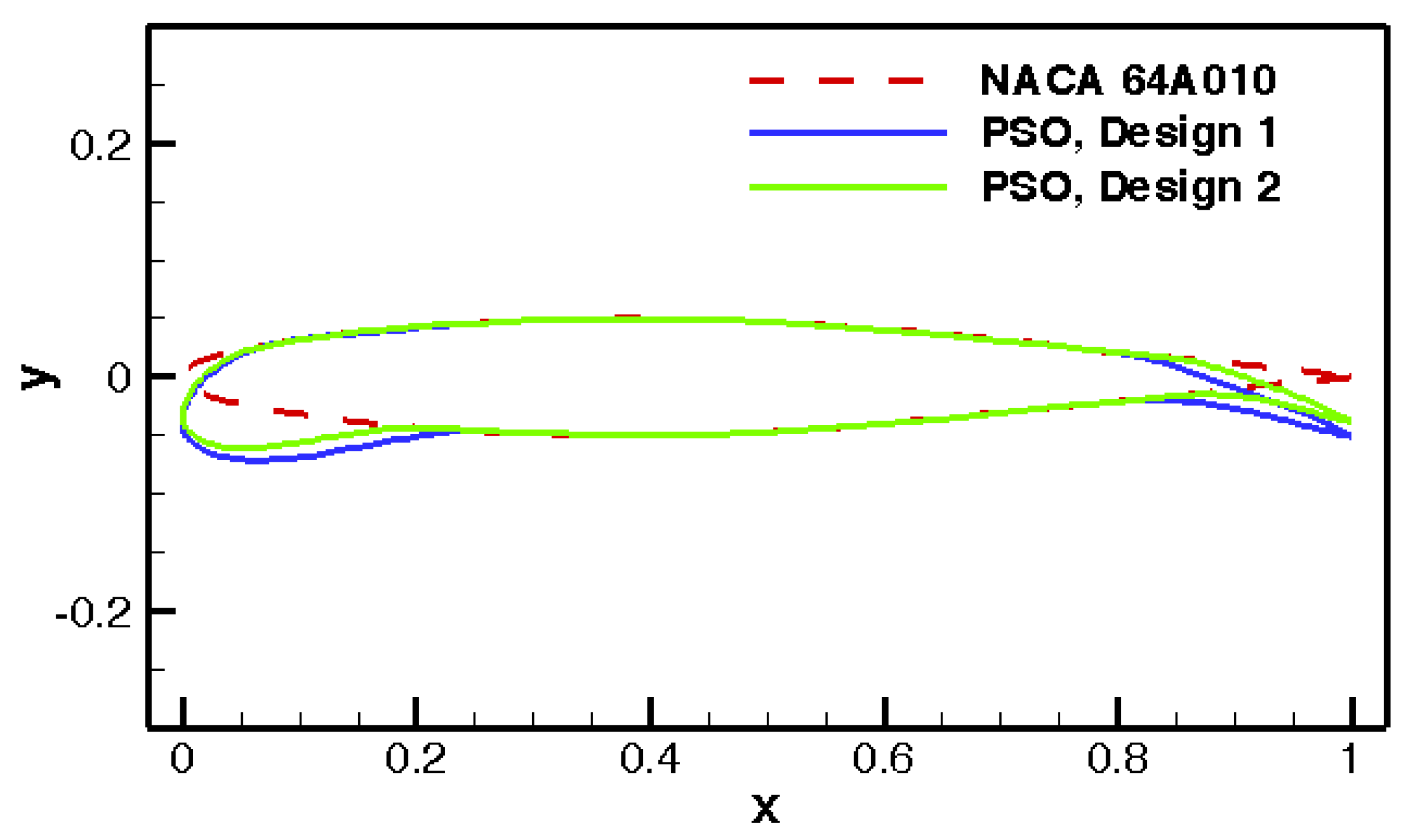
The results of this more conservative approach for the three optimization algorithms are summarized in
Table 3. It can be observed that, keeping the same number of generations, the PSO algorithm again provides the airfoil with the maximum C
L,max. Compared to the more “aggressive” approach, there is a 2.25% reduction in the C
L,max plus the fact that the double number of generations are needed to reach the optimum design. On the other hand, smaller deformations are required to achieve that C
L,max, as shown in
Table 4.
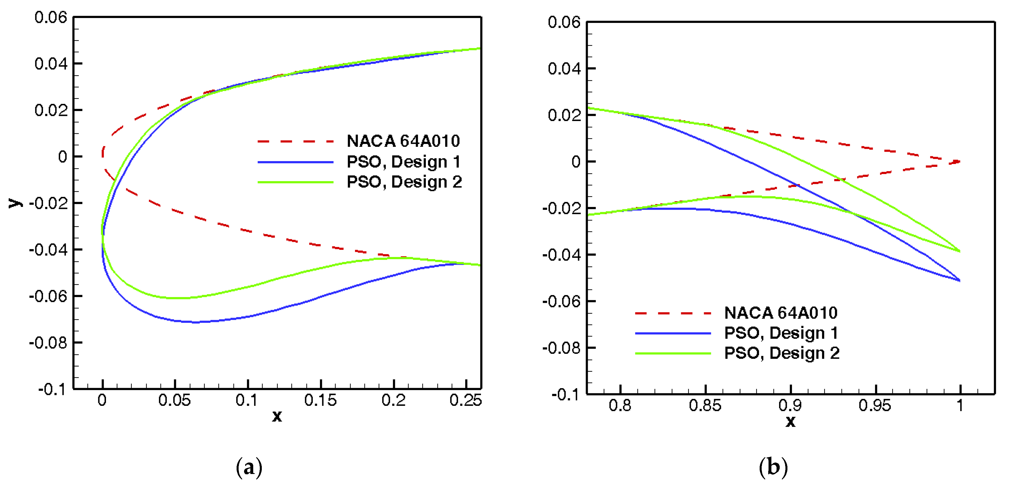
Figure 6 compares the two different designs, whilst
Figure 7a,b focuses on the deformed parts at the LE and TE regions, respectively. These plots confirm the smallest deformations when the more conservative setup is used. It should be noted though, that in both setups, proper constraints ensuring the continuity of the geometry have been imposed, as described in
Section 2. The more conservative design could prove to be more efficient in cases where limitations of the permitted deformations are imposed by structural analysis. In the present work, such an analysis is not included, therefore the more aggressive design (design 1) with the higher C
L,max is adopted in the sequel.
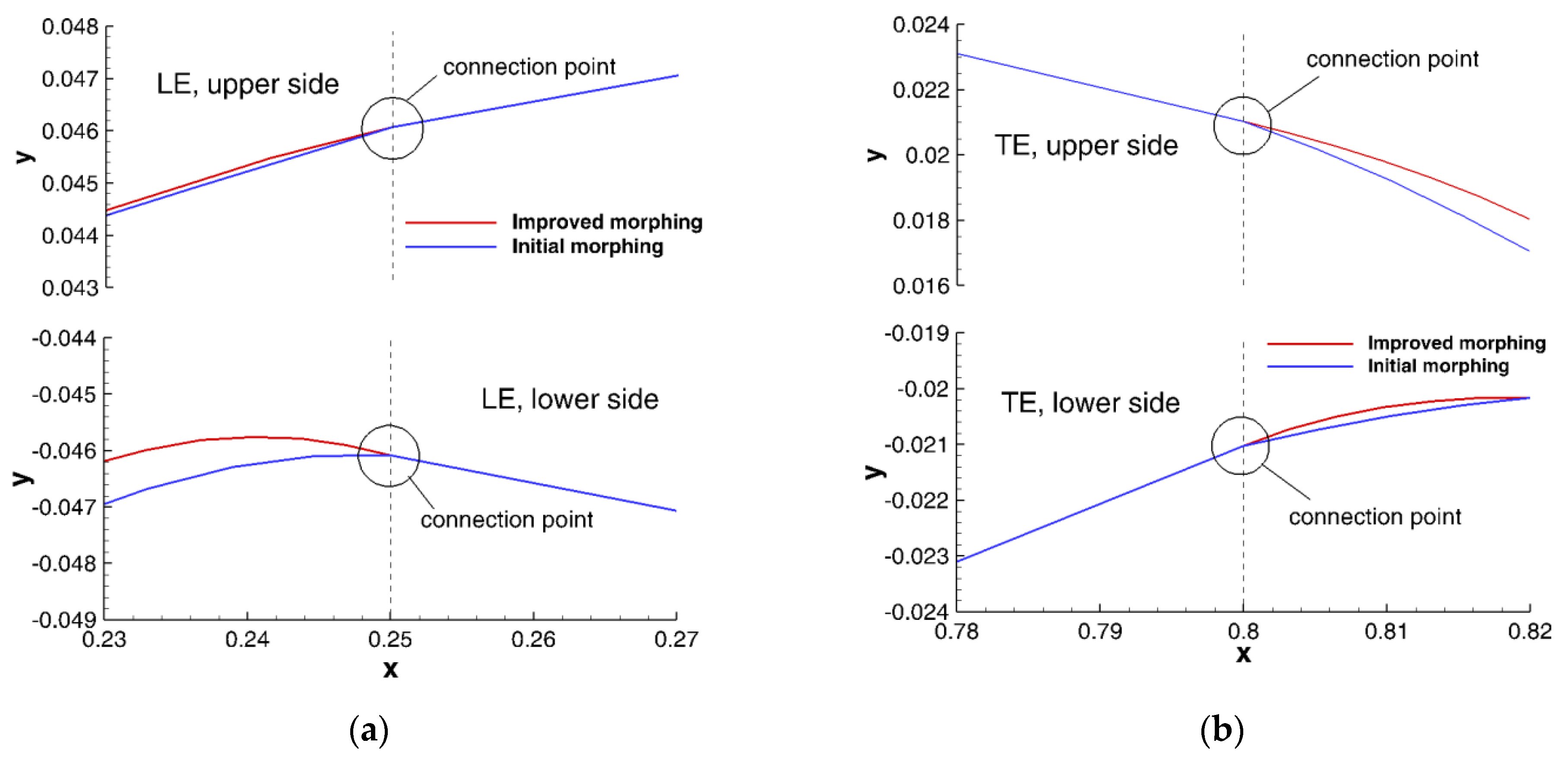
A closer look at the connection points between the morphing and the undeformed parts of the airfoil reveals small discontinuities of the geometry, more evident at the lower side of the LE region and the upper side of the TE region. These discontinuities can be smoothed out by imposing additional fixed control points between those already fixed (green points in
Figure 2) and the points with numbers 1, 7, 8, and 14 (
Figure 2). The effect of such a treatment is shown in
Figure 8. It is observed that a smoother geometry is achieved locally, through the addition of the intermediate control points, which keep the continuity of the first derivative at the connections. As expected, the effect is more pronounced at the lower side of the LE and the upper side of the TE, where the larger discontinuities were present.
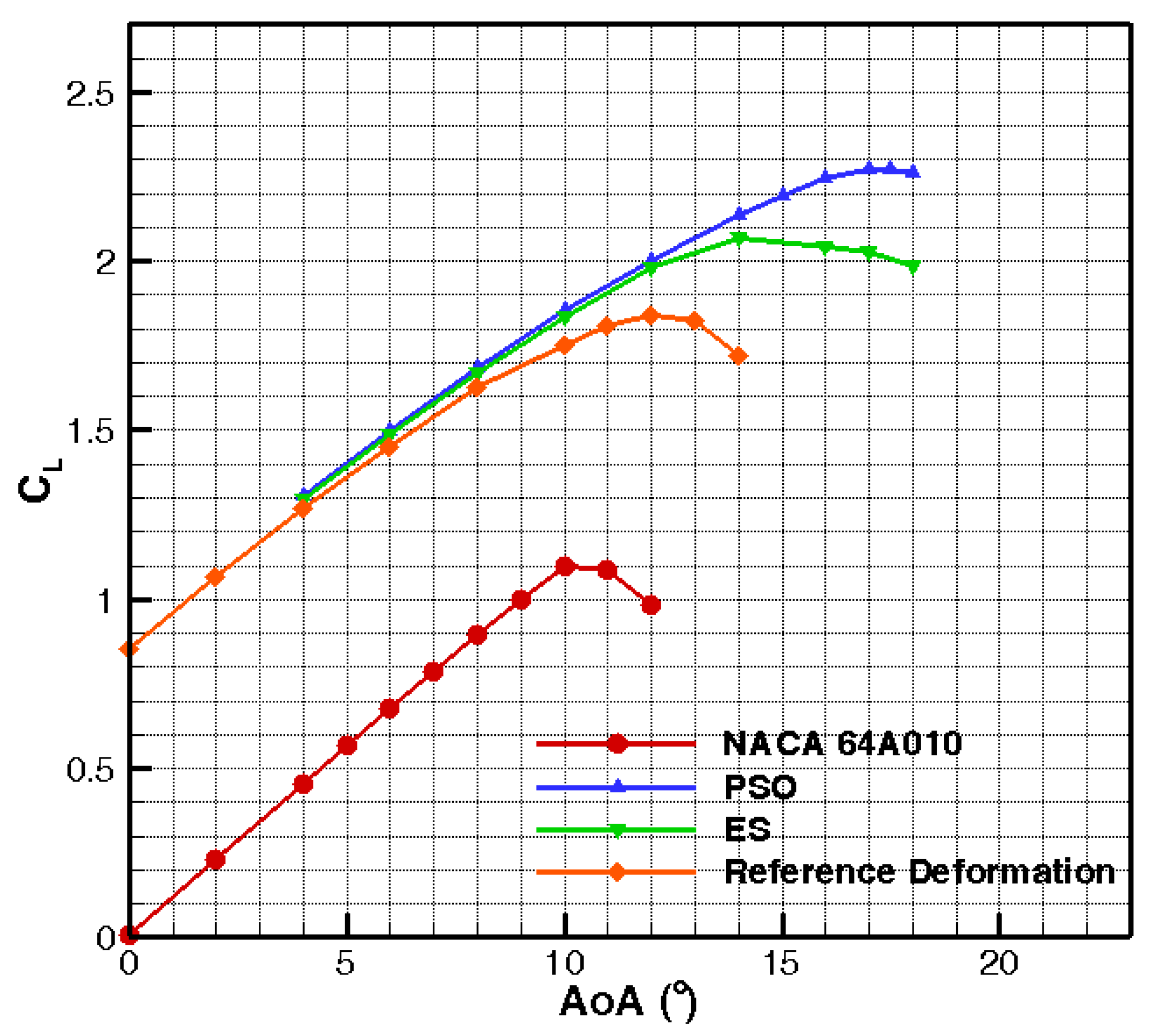
The effect of the combined LE/TE morphing on the C
L-AoA polars is depicted in
Figure 9. The airfoils designed from the PSO and ES algorithms are compared against the initial NACA 64A010 airfoil and the one with the reference deformation, which was used as a starting point for the definition of the control points’ intervals (
Figure 3). First, stall is delayed, occurring at a higher angle of attack, in comparison to both the original NACA 64A010 and the reference deformation airfoils (17° for PSO, 14° for ES, 12° for reference deformation, 10° for original NACA 64A010). Second, C
L,max increases considerably, from 1.1 (original NACA 64A010) to 2.27 and 2.07 for the PSO and the ES airfoils, respectively. A significant increase is also observed with respect to the reference deformation airfoil that presents a C
L,max of 1.84.
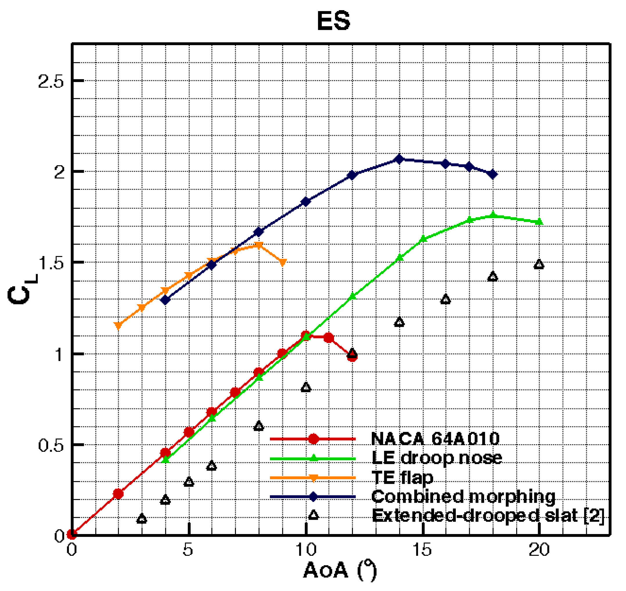
In order to distinguish the effect of LE and TE morphing on the overall lift change, additional optimizations are performed applying each one of the two morphings separately. Both PSO and ES algorithm are employed, while the maximum number of generations is kept the same with the previous analyses (four generations for PSO and eight generations for ES), to derive results directly comparable with those of the combined LE/TE shape optimization.
When only LE droop nose is applied, stall is significantly delayed (20° for PSO-airfoil and at 18° for ES-airfoil compared to 10° for the original airfoil), whilst the zero-lift angle of attack remains almost unchanged (similar to the effect of a multi-element slat). As a result, a 60–80% increase (depending on the optimization method used) of the CL,max is achieved.
When only TE flap is applied, the effective camber line increase at the TE region results in the shifting of the entire CL polar towards lower AoA (similar again to the effect of a multi element flap). In this case, stall occurs at a lower angle of attack (8° for both airfoils). Furthermore, the slowing down in the rate of the lift increase starts earlier in the morphed airfoil as compared to the baseline undeformed shape. This is an indication of an earlier separation of the flow at the TE region, triggered by the local effect on pressure by the high geometric curvature. The CL,max increase in this case is limited to 45%.
When both morphing mechanisms are applied, the two effects are superimposed (though not linearly) and the overall increase in CL,max is maximized (88–107%).
Measurements of the lift coefficient polar for an extended and drooped slat configuration on the same NACA 64A010 are also presented in
Figure 10 and
Figure 11. The Mach number and the flap deployment of the experiment [
1] are 0.25 and 14.5°, respectively, very close to the simulated setup. The comparison shows a significant improvement of the C
L,max when the suggested droop nose morphing is applied, even if the lower Reynolds number of the experiment is considered (3.5 × 10
6).
Percentages of C
L,max increase for the individual LE droop nose and TE flap, as well as for the combined morphing are summarized in
Table 5. The C
L,max increase with respect to the reference deformation airfoil (combined morphing) is 23.5% and 12.3% for the PSO and ES airfoils, respectively.
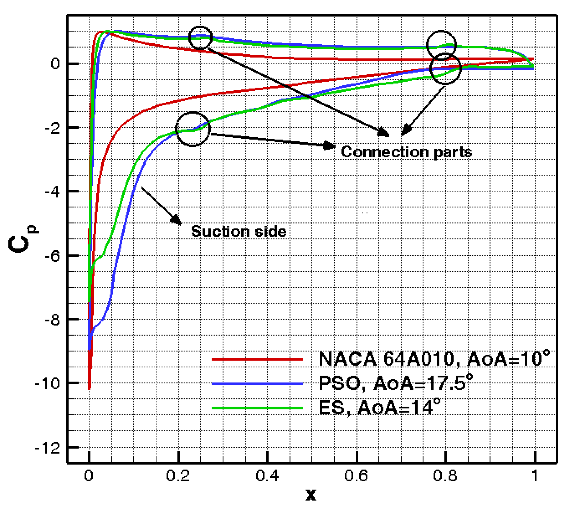
A closer look at the pressure distribution (presented in
Figure 12) around the morphed shapes and the undeformed baseline NACA 64A010 can provide information for the physical interpretation of the attained C
L,max increase. Pressure distributions are plotted for AoAs corresponding to the maximum value of the lift coefficient. This is at 17.5° and 14° for the morphed shapes predicted by PSO and ES algorithms, respectively, and 10° for the baseline NACA 64A010 (see
Figure 9). Apparently, the larger extent of the high under-pressure pocket on the suction side in the vicinity of the LE region drives the increase in the maximum C
L. The PSO airfoil exhibits a suction pressure peak of about 25% higher than that of the ES airfoil. This explains the higher C
L,max value obtained by this airfoil. Although the suction peak of the baseline airfoil is larger than those of both morphed shapes, the pressure of the baseline airfoil quickly recovers within a very short distance (less than 5%) from the LE point. The under-pressure of the morphed shapes remains high up to 10% of the chord distance from the LE. It is noted that for both morphed shapes, at the C
Lmax AoA, the flow remains almost attached over the whole suction side. A limited separation is obtained for both morphed airfoils at about 80% of the chord (seen as a plateau of the pressure coefficient beyond this chordwise position). Another interesting observation is related to the pressure variation at the connection points between the deformed and undeformed airfoil parts, where it is desirable to avoid steep flow disturbances. The plots of the pressure coefficient in
Figure 12 do not present significant irregularities, confirming that the imposed curvature and slope constraints, integrated into the optimization procedure, prevent the occurrence of significant geometric discontinuities. Moreover, in the PSO airfoil, the additional fixed control points between the morphed and the undeformed part improve the continuity of the geometry at the connections (see
Figure 8), and this effect is also reflected on the C
P distribution (at least at the two connection points of the suction side and the TE connection point of the pressure side). It is noted that compared to the ES, the PSO airfoil presents a smoother pressure distribution in the vicinity of the LE connection point on both sides (upper and lower), despite the larger deformation undergone by the PSO morphed airfoil at the LE region.
4. Validation with a High Fidelity Solver
To verify the results obtained by Foil2w, the flow around the modified geometries is also simulated using MaPFlow, a CFD URANS solver. In both codes, transition modeling is realized using the same model e
N. For the CFD simulations, the computational grid is generated using the ANSYS ICEM software [
29]. Special care is taken to generate a grid sufficiently dense within the boundary layer region and in the vicinity of the LE and TE regions. The distance of the first node from the surface is 10
−6 chords (y
+ ≈ 1). In
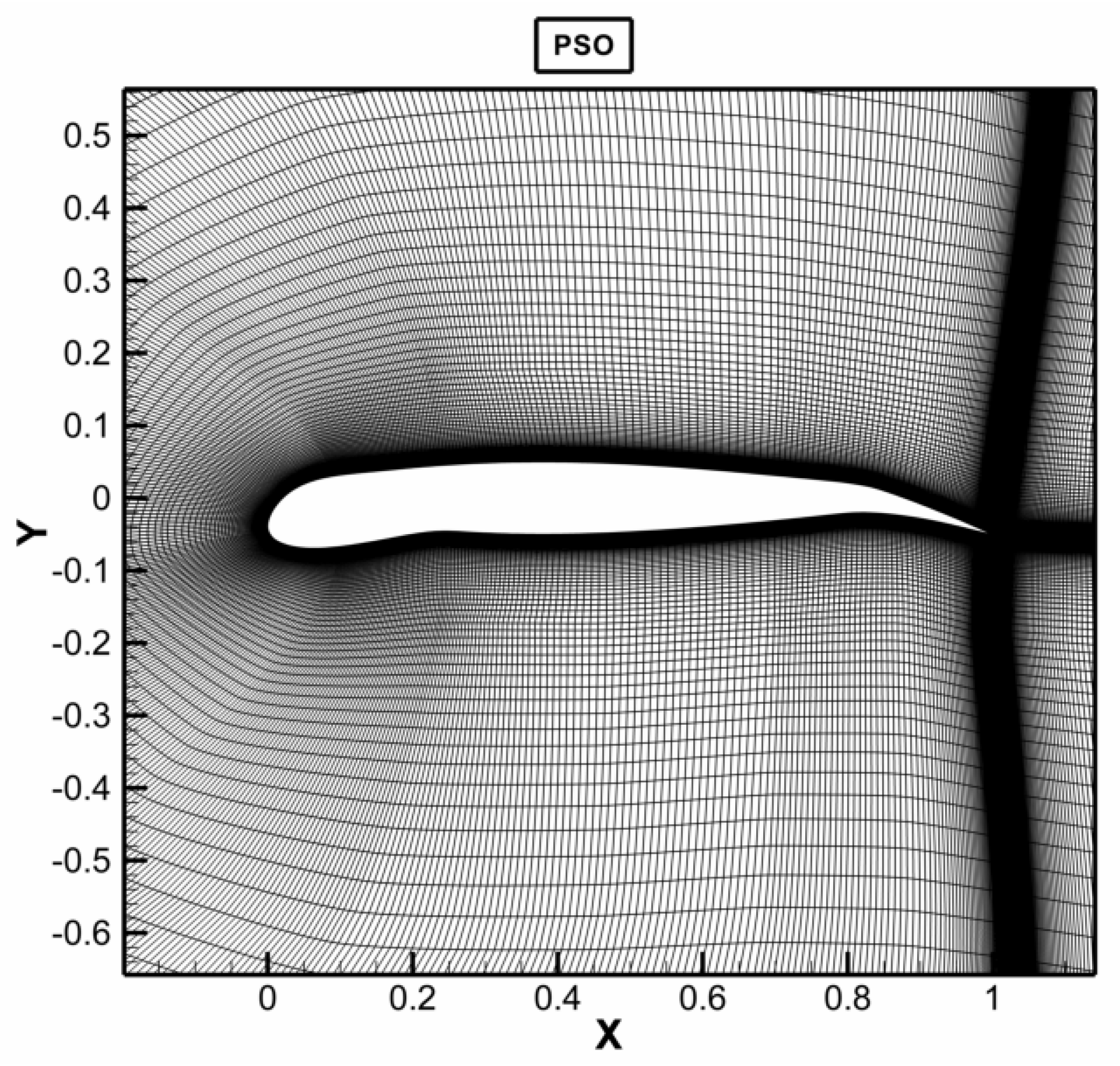
Figure 13, the mesh for the PSO-airfoil is depicted, whilst a similar mesh was created for the ES-airfoil. It consists of 606 wrap around nodes and 180 nodes in the normal to the surface direction. Out of the 180 nodes in the normal direction, 120 are distributed from the surface up to a distance of 0.13 chords using a geometrical progress with ratio 1.08.
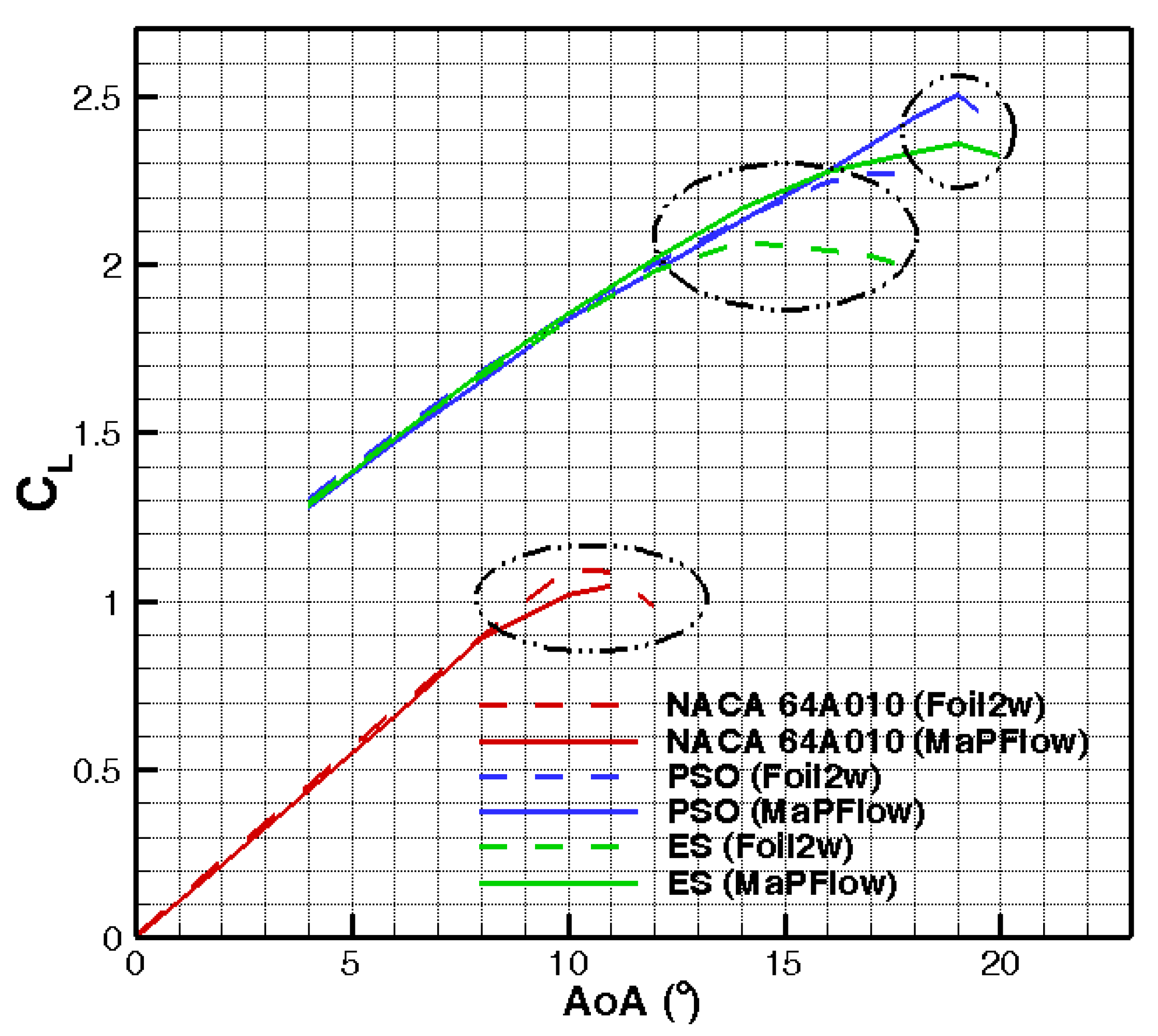
Figure 14 compares the MaPFlow and Foil2w predictions of the C
L-AoA polars for the optimized morphed airfoils. The MaPFlow and Foil2w polars for the original airfoil are also presented in the plot. Higher C
L,max values are systematically predicted by the CFD solver for the morphed airfoils, although the opposite applies for the baseline NACA 64A010. In general, compared to the original airfoil, the differences between the two codes increase, as the airfoil geometry is deformed. This is due to the fact that, as the geometry becomes more complex, and taking into account that transitional effects are included, the results become more sensitive to the simulation of viscous flow phenomena, such as the prediction of the transition locations and the appearance of separation. The maximum lift coefficient increases from 1.1 to 2.5 and 2.3 for the PSO and ES airfoils, respectively. This is due to the fact that in the CFD simulations stall takes place at higher angles of attack (19° for both PSO and ES). It is noticeable that in MaPFlow predictions the ES airfoil exhibits higher C
L values than the PSO airfoil at AoAs in the range 5–15°, below the C
L,max AoA. In aeronautical applications, this region is outside the operation points of interest and it is probable that morphing is applied differently at the lower AoAs. In the case of wind energy applications, though, the operational region is broader indicating that a larger part of the polar should be taken into account.
In
Table 6, percentages of the maximum lift coefficient increase for the designed airfoils, as predicted using Foil2w and MaPFlow, are summarized and compared. It is underlined that CFD predictions indicate that PSO-airfoil reaches a 140% increase in C
L,max, while ES-airfoil reaches a 125% increase. Therefore, MaPFlow exhibits an even higher increase in C
L,max (more than 100%), suggesting that the results of the optimization using the lower fidelity Foil2w solver are conservative at least for the particular airfoil studied in the present work. It is worth noting that contrary to the morphed airfoils, the C
Lmax predicted by the CFD code for the baseline airfoil is slightly lower than the one provided by Foil2w.
Velocity contour plots around the PSO airfoil are depicted in
Figure 15, at the AoA where the maximum value of lift coefficient occurs (19°). The flow patterns of
Figure 15 confirm the discussion made in the previous section. The concurrent drooping and thickening of the airfoil nose over its forward 10% leads to a smoother acceleration of the boundary layer (lower pressure gradient), which is retained over a larger portion of the suction side forming a high velocity pocket (flow velocities 2.5 times higher than the free stream velocity) up to 10–20% of the chord. Furthermore, the overall flattening of the whole suction surface, driven by the thickening of the forward 7–20% of the LE region leads to retarded separation of the flow, which, as also predicted by Foil2w code, at this high AoA (19°) is limited to the aft 20% of the airfoil section (low velocity pocket in the vicinity of the morphed TE part). Flow velocities depicted in the contour plot of
Figure 15 exhibit a smooth variation at the connection parts, confirming again that the geometric constraints imposed in the optimization loop prevent geometric irregularities.
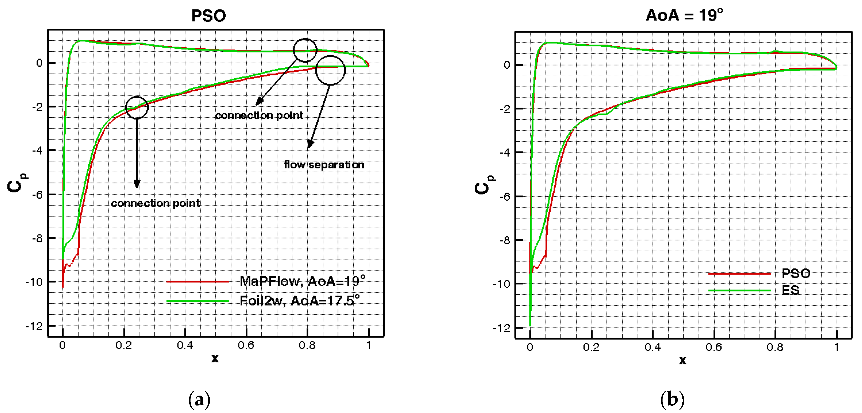
In
Figure 16a, the pressure coefficient distributions predicted by Foil2w and MaPFlow code at the C
Lmax AoA of the PSO airfoil are compared (19° for MaPFlow and 17.5° for Foil2w). Comparing the two distributions, two differences are distinct: (a) MaPFlow predicts slightly higher suction peak resulting in a higher C
L,max and (b) Foil2w predicts a slightly more extended flow separation at the TE region (pressure plateau at the rear part of the airfoil) even at the lower angle of attack of 17.5°. In
Figure 16b, the pressure distribution predicted by MaPFlow is presented for the two optimized airfoils at the C
L,max AoA (angle of C
L,max 19° for both the PSO and the ES airfoils). Results of
Figure 16b (predicted by MaPFlow code) are qualitatively very similar to those of
Figure 12 (predicted by Foil2w). The main difference is that Foil2w predicts much lower suction peak for the ES airfoil, which justifies the lower C
L,max predicted by the same code for the particular airfoil. MaPFlow predictions confirm that disturbance of the pressure at the connection points is lower for the PSO airfoil.
The whole design process has been based on the C
L,max optimization, which is critical during the take-off and landing segments of the flight. However, another important factor, especially during the take-off procedure, is the aerodynamic performance (C
L/C
D), which is related directly to the fuel consumption of the aircraft. Most commercial transport aircraft are optimized to fly with a small incidence at an altitude close to 11,000 m. While climbing to or descending from this optimal altitude the aircraft will travel with a large incidence, therefore, will operate inefficiently and as a result will consume a lot of fuel. It is expected that the designed airfoils will produce increased drag because of the highly deformed shape at the droop nose LE. This is confirmed by the MaPFlow predictions (
Table 7) which suggest larger C
D values for the morphed airfoils at the C
L,max AoA. However, the substantial lift increase mentioned in the above analysis compensates for the drag increase, resulting in improved aerodynamic performance as reported in
Table 7. This confirms the overall aerodynamic effectiveness of the designed airfoils.
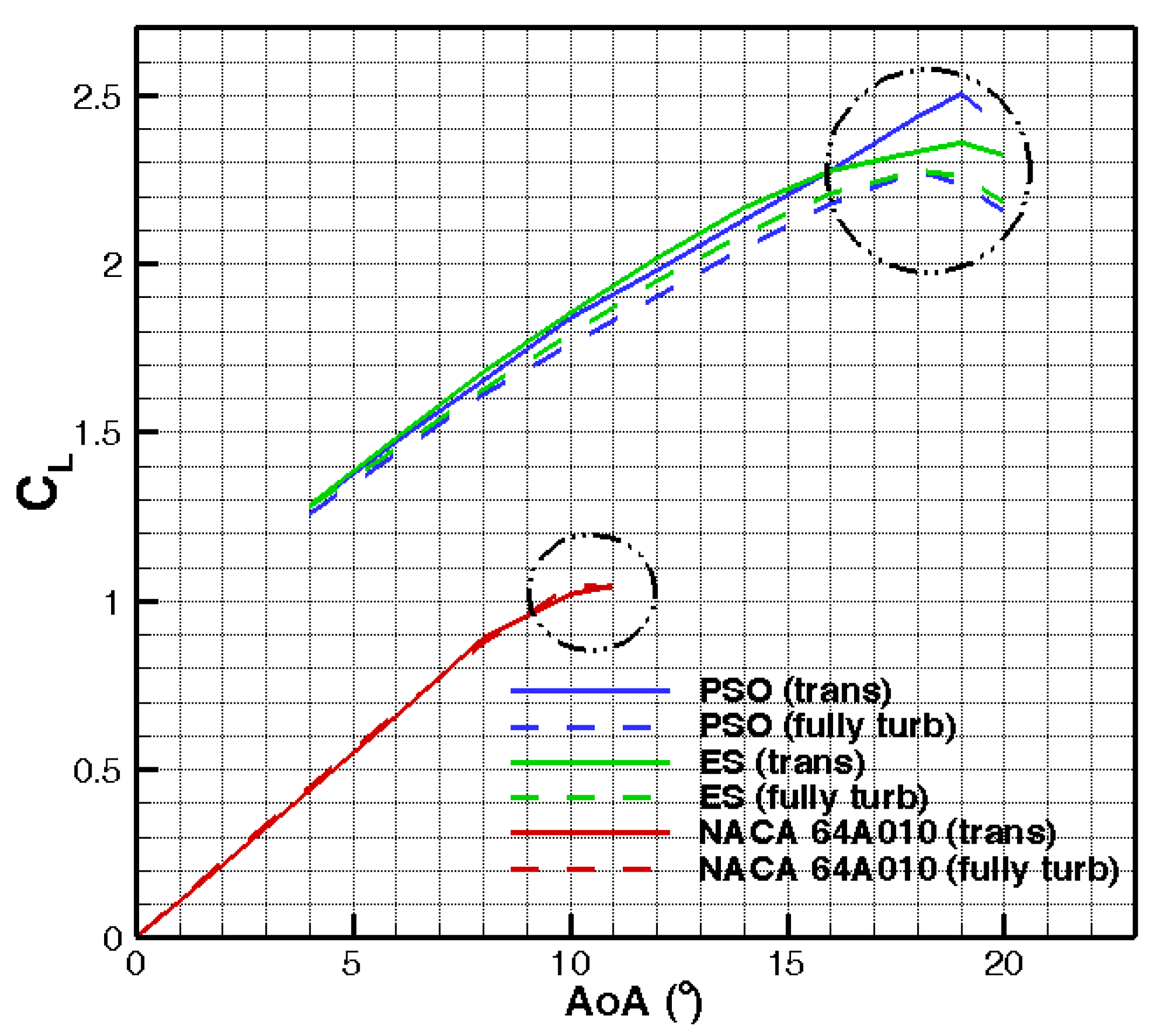
In all aforementioned simulations, transitional conditions are considered. Potential increase of the surface roughness would force transition of the flow from laminar to turbulent to occur earlier, which generally leads to reduced maximum lift. In order to assess performance deterioration of the morphed sections due to earlier (forced) transition, fully turbulent flow simulations are performed with MaPFlow code. As seen in the marked regions of
Figure 17 changing flow conditions from transitional to fully turbulent does not significantly affect the C
L,max value of the baseline NACA 64A010 airfoil, but causes an appreciable reduction in the C
L,max of both PSO and ES optimized morphed airfoils. Moreover, the C
L,max AoA decreases by 1° for both airfoils. Overall, as opposed to the transitional case, in turbulent flow conditions the ES airfoil outperforms the PSO airfoil over the whole range of the simulated AoAs. As noted above, this effect could be important to wind energy applications, in which the blade airfoil encounters a broad range of AoAs.
Table 8 summarizes the C
L,max predictions for transitional and turbulent conditions and the relative increase with respect to the baseline airfoil. Changing from transitional to fully turbulent conditions mitigates the relative increase of 139% and 126%, for the PSO and ES airfoils, respectively, to the same level of 118% for both airfoils.
5. Discussion
In the present study, a methodology for designing high-lift mechanisms for aircraft wings is developed, applying a combination of LE droop nose and TE flap morphing. Airfoils of increased maximum lift are produced through an optimization process, where smooth polynomial curves approximate the morphing parts in the LE and TE regions of the airfoil, while a viscous-inviscid fast interaction code is used for the prediction of the aerodynamic characteristics. Results indicate that significant increase in maximum lift coefficient and stall angles of attack are achievable. The contribution of each morphing mechanism (LE droop nose, TE flap) to the total CL,max increase is investigated. When only LE droop nose is applied stall is delayed and, as a result, lift coefficient increases allowing the airfoil to operate at higher angles of attack. On the other hand, when only TE flap is applied the effective camber line increase at the TE region results in the shifting of the entire CL polar towards lower AoA. The entire level of the CL curve increases, but stall occurs at lower AoA. The combined effect is a delayed stall along with a shift of the CL curve to a higher level.
The above conclusions are verified using a high fidelity CFD solver. CFD predictions exhibit an even higher CL,max increase due to delayed stall and higher pressure peaks at the suction side of the LE, suggesting that the optimization results derived with the fast viscous-inviscid interaction code are conservative at least for the current airfoil study. The imposed curvature and inclination constraints prevent the appearance of geometric irregularities and flow disturbances at the connections between the undeformed and the morphing parts. This is reflected on the predicted smooth pressure distributions and the velocity contours. The present work focuses on the achievable increase of the maximum lift, which is desirable during take-off and landing flight procedures; aerodynamic performance is not considered in the optimization process. However, the predictions of the CFD solver demonstrate that although morphing airfoils produce an increased drag, they are still capable of operating with much higher aerodynamic performance (CL/CD). This interesting outcome ensures the overall aerodynamic effectiveness of the designed airfoils and indicates the potential of the developed optimization methodology to be applied to other contiguous technologies, such as wind energy, where maximization of CL/CD is likely to be the most relevant design objective for maximum energy yield.
Finally, fully turbulent flow simulations are performed to investigate the effect of a potential increase of the surface roughness. As expected, fully turbulent calculations predict lower values of the maximum lift. It is observed that in fully turbulent conditions, PSO and ES optimized airfoils produce a similar CL,max, whilst in transitional conditions, the PSO airfoil produces a considerably higher CL,max. Therefore, changing from transitional to turbulent conditions mitigates maximum lift increase to the same level for both airfoils.


 ,
, 


