
Kernel Point Convolution LSTM Networks for Radar Point Cloud Segmentation


Abstract
1. Introduction
- Radar signals are affected significantly less by rain or fog than lidar [3].
- Radar sensors measure the radial velocity of surrounding objects directly.
- The spatial resolution of production radar sensors is lower than that of lidar [3].
- Current production radar sensors do not measure the elevation component of the radar returns.
- Several processing steps are necessary to obtain a radar point cloud from the raw sensor signals. These processing steps are based on additional assumptions, e.g., prioritizing moving objects, which may not lead to the desired point cloud signal in all environmental conditions.
- The paper adapts KPConv network architectures for radar point cloud data processing.
- The paper proposes modified LSTM network architectures to process irregular radar point cloud input data. The advantages and disadvantages of different time modelling and association techniques are discussed. However, an empirical study on public radar data does not motivate a preferred network architecture.
- The paper analyzes publicly available radar data for autonomous driving. It concludes that the data quality of the public data is not sufficient. Furthermore, it proposes which key points to consider when composing a radar data set for autonomous driving research.
- The code for this research is released to the public to make it adaptable to further use cases.
2. Related Work
2.1. Lidar Point Cloud Segmentation
2.2. Lidar Object Detection
2.3. Radar Point Cloud Processing
3. Methodology
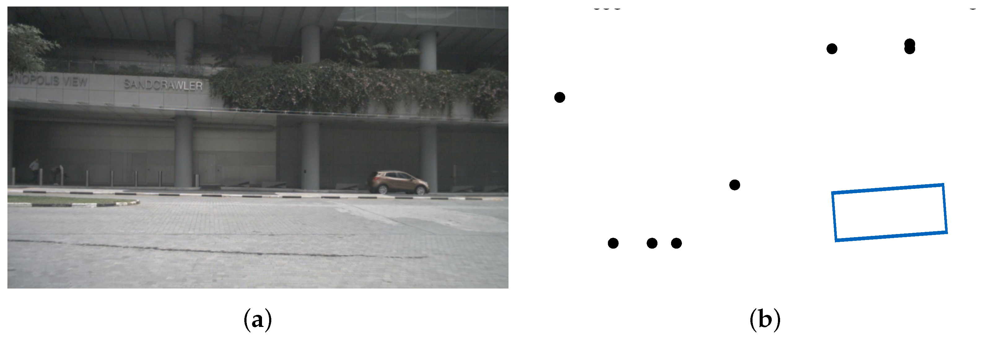
- Data Availability: In contrast to lidar research, where a vast amount of labeled data is publicly available, the access to radar data is more restricted. Accurately labeled data is the basis for any successful supervised learning model, which means that reduced data availability could be one reason for the smaller amount of research work in this area. A more detailed view of radar data available to the public is given in Section 5.2.
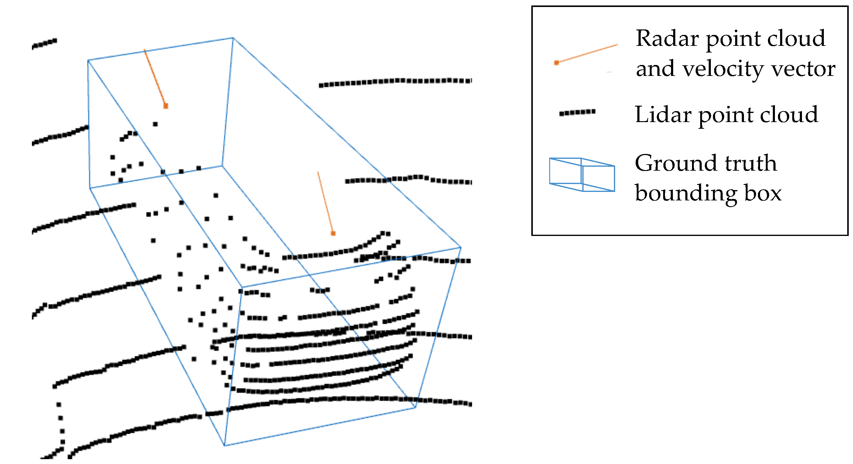
- Data Level: Due to the sensor principle of the radar, a variety of intermediate processing stages occur before the raw receive signal is converted into object proposals.The unprocessed low-level raw antenna signals theoretically contain the most information; however, there are no methods of labeling data on this abstraction level for object categories. Additionally, depending on the antenna characteristics and configuration, the data would differ a lot for different radar types, which would require a specific learning approach for different sensor hardware designs. Consequently, to the best of our knowledge, no one-step learning approach exists for classifying objects directly on the raw antenna signals.One can perform object detection at the radar cube level or on any of its 2D projections, e.g., range-azimuth plot. However, data labeling of this 3D representation (2D location + velocity) would still be a tedious task. [22] performs the labeling by extracting data from the cube at manually labeled point target locations. However, in this way the label quality can only approximate the ground-truth, as the point target might not include all raw signals that originate from an object. Furthermore, the point targets only represent a compression of the radar signal, which means that the point signal cannot be re-projected precisely on the cube-level signal. To our knowledge, no full 3D cube-level radar data set has been released to the public. However, due to the high informativeness and the similarity to image data, which is heavily processed with learning-based techniques, the cube-level data is an interesting use case for future deep-learning research on radar data.Point level data is the most explored data level for deep learning on radar data. It represents a compromise between data informativeness and data amount. Due to the similarity to lidar point cloud data, algorithms can be transferred from the lidar domain to the radar domain. This work operates on point level radar data. We benchmark our models on the public nuScenes data set [2], which includes labeled point cloud radar data.
- Data Sparsity: For lidar data processing, both grid and point-based approaches, are used in the state of the art. Similar to [20], we argue that for radar data, a point-based approach is more feasible than the intermediate grid representation as most of the grid cells would remain empty. For fusion approaches of radar data with denser data such as images or lidar both grid-based and point-based approaches [24,25,26], might be suitable. This work presents a point-based approach. To the best of our knowledge, we are the first to adapt the KPConv architecture for radar point cloud data.
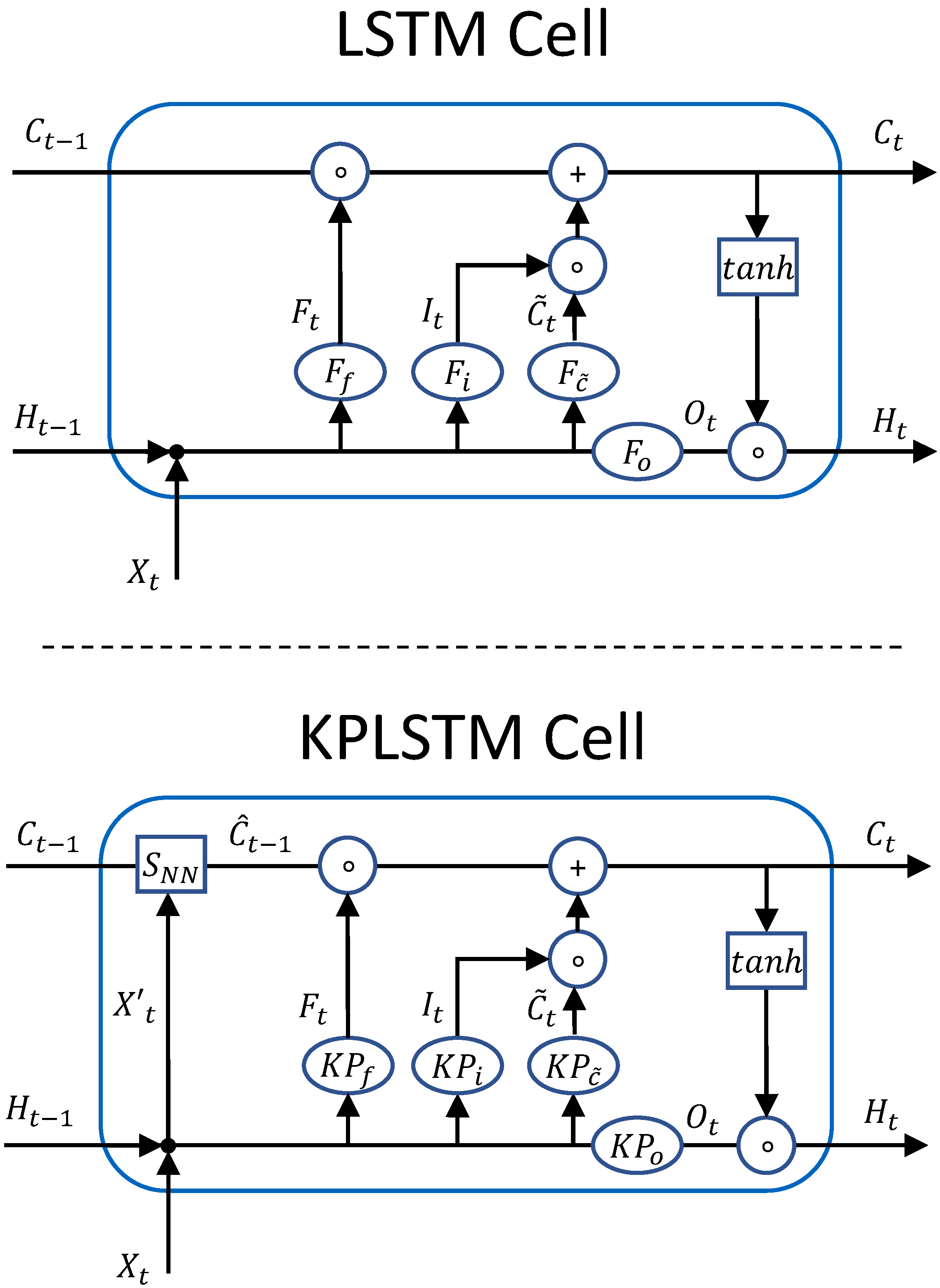
- Time Dependency: Due to the low spatial resolution of radar sensors, the time domain plays an important role in radar processing. Current production radar systems track point level detections over several timeframes before recognizing a track as an object. This decreases the number of false positive object detections due to clutter. These false positives would otherwise be harmful to driver assistant systems such as adaptive cruise control (ACC) or emergency brake assist. In the literature, approaches that use the time domain in learning models such as simple LSTM cells or memory point clouds have proven successful for radar data processing. This paper integrates KPConv layers into an LSTM cell, which we call KPConv-based LSTM (KPLSTM). In this way, we can encode the time dependency for points individually. Additionally, we combine KPConv encoding with LSTM and ConvLSTM cells [27] in the latent space to integrate the time domain in the model on a global feature level.
- Moving Object Recognition: In addition to the time dependency, production applications only react to moving objects, as the amount of clutter among the static points causes additional challenges for the processing. It is desired to bring radar processing to a level of maturity to detect static objects just as with the lidar sensor. However, the research above shows that the focus is still mainly on the moving object case. Even in the simplified moving objects scenario, the detections are only reliable enough for simplified use cases, such as vehicle following in the ACC case. In this work, we evaluate our network for both static and dynamic cases and show the disadvantages of the radar for the complex static scenarios.
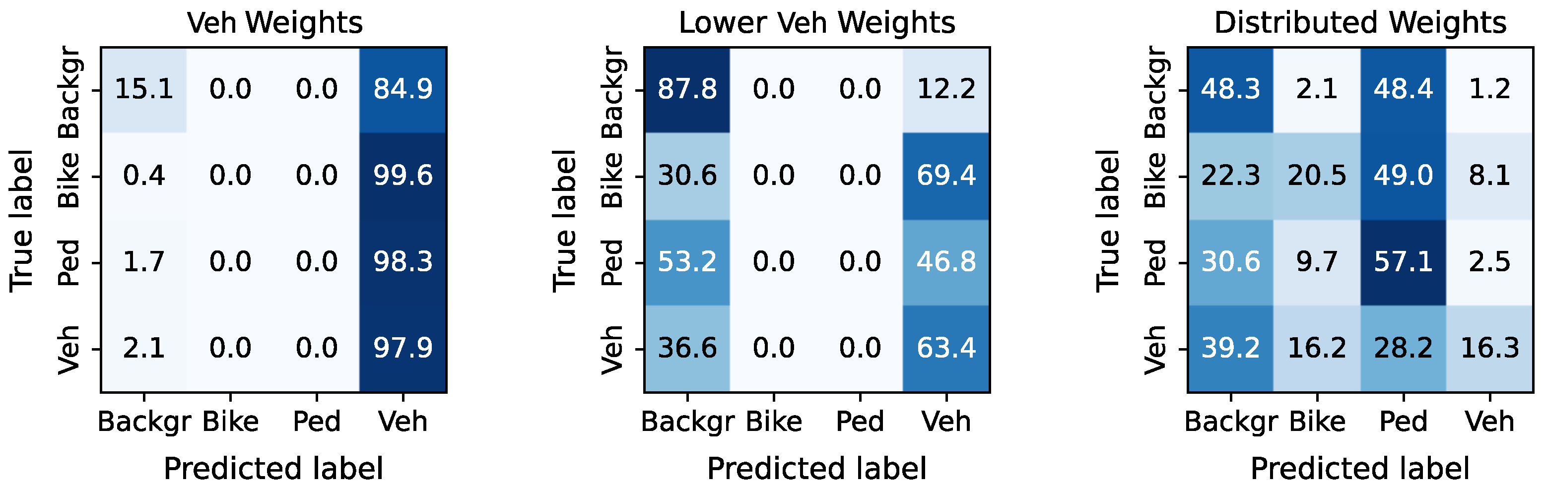
- One-vs-all Classification: Due to the difficulties in creating reliant object detections from radar data, one compensation strategy is the simplification of the scenarios. In the literature, one-vs-all classification are an efficient way to simplify the training use case, while keeping a relevant task in focus. This paper shows the results for different training configurations and their impact on the segmentation performance.
3.1. Model
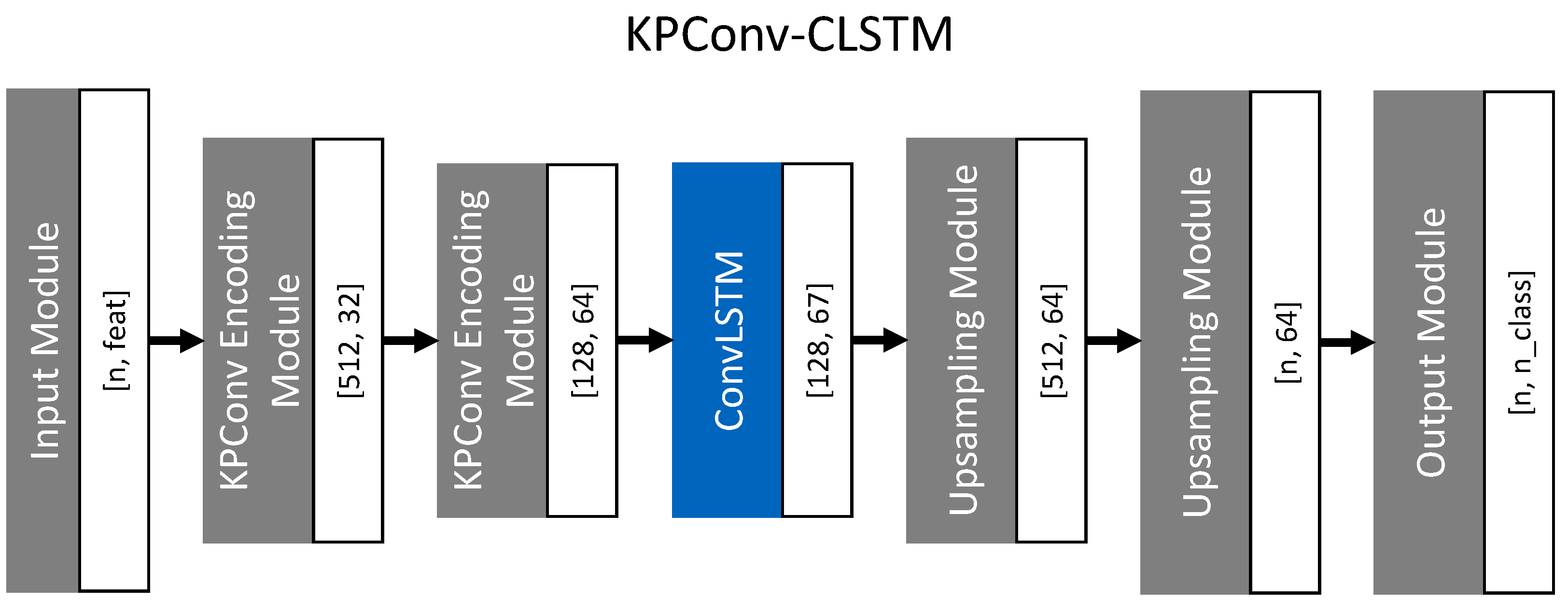
3.2. KPConv with LSTM Cells in Latent Space
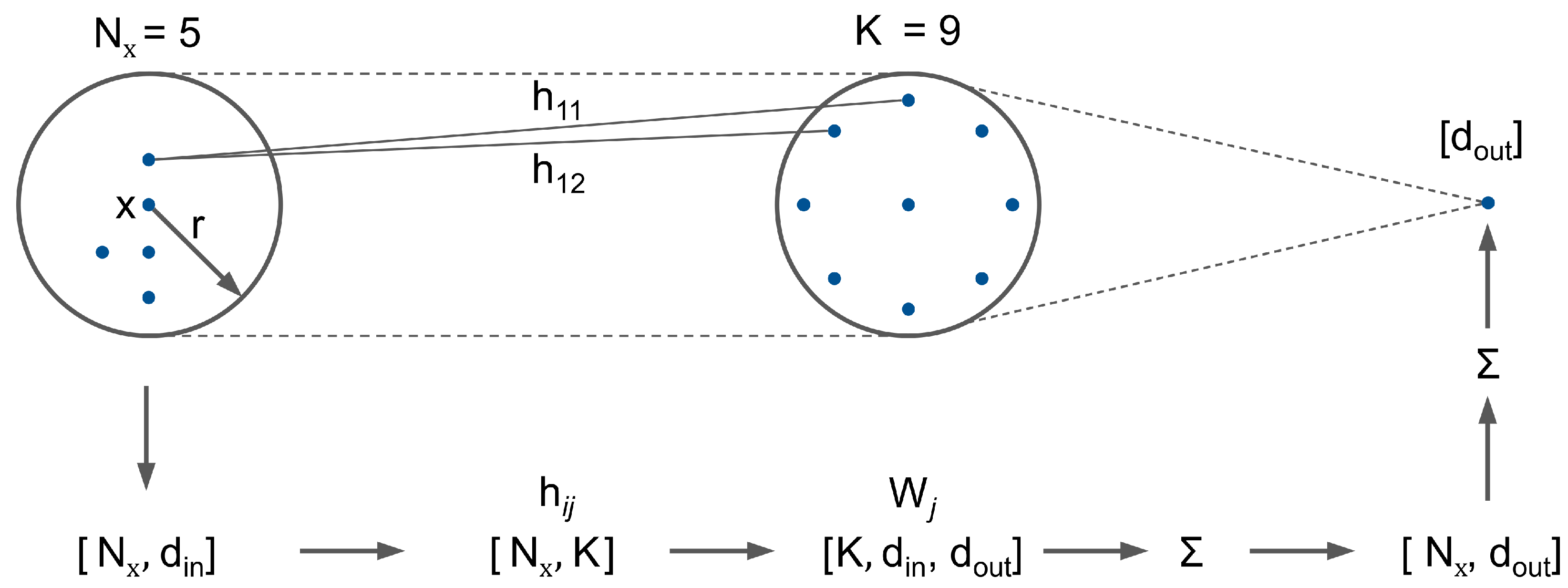
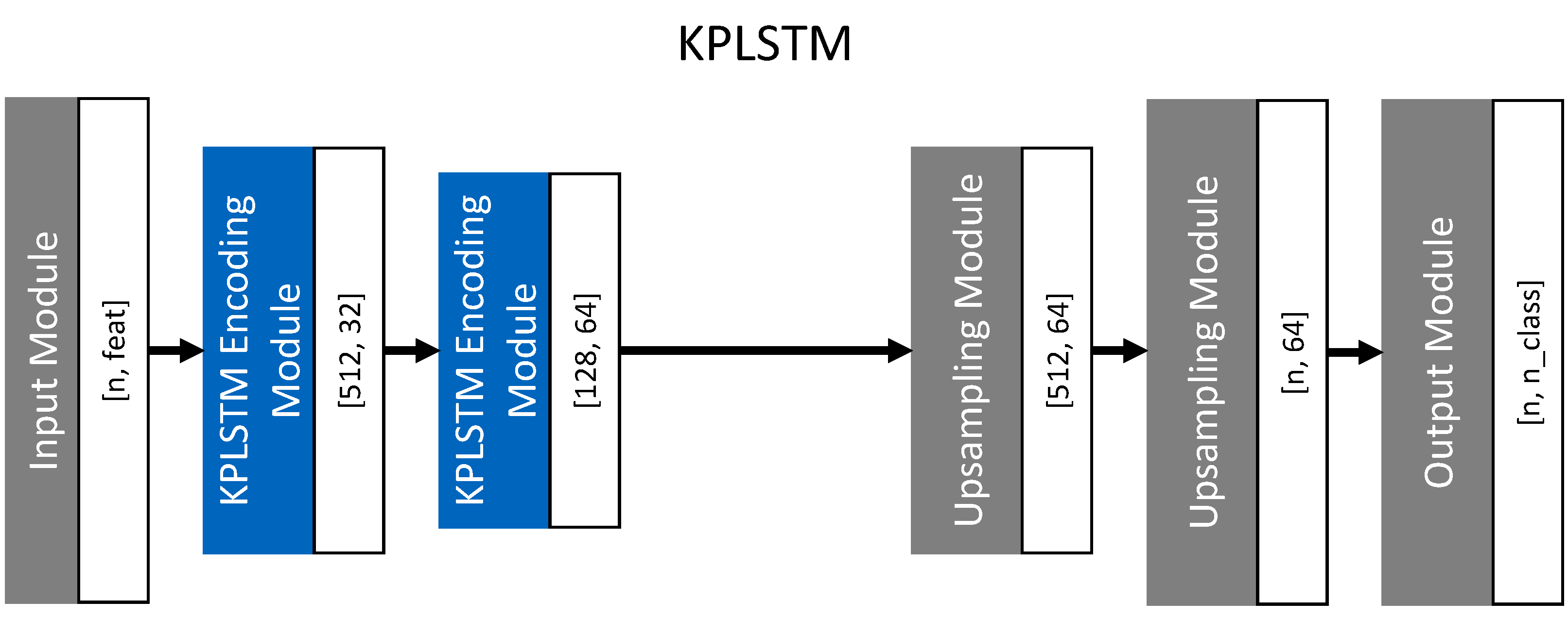
3.3. KPLSTM
3.4. Data Processing
3.5. Training
4. Evaluation
4.1. Traffic Data Set
4.2. All Vehicle Data Set
4.3. Moving Vehicle Data Set
4.4. Velocity Input Feature Study
5. Discussion
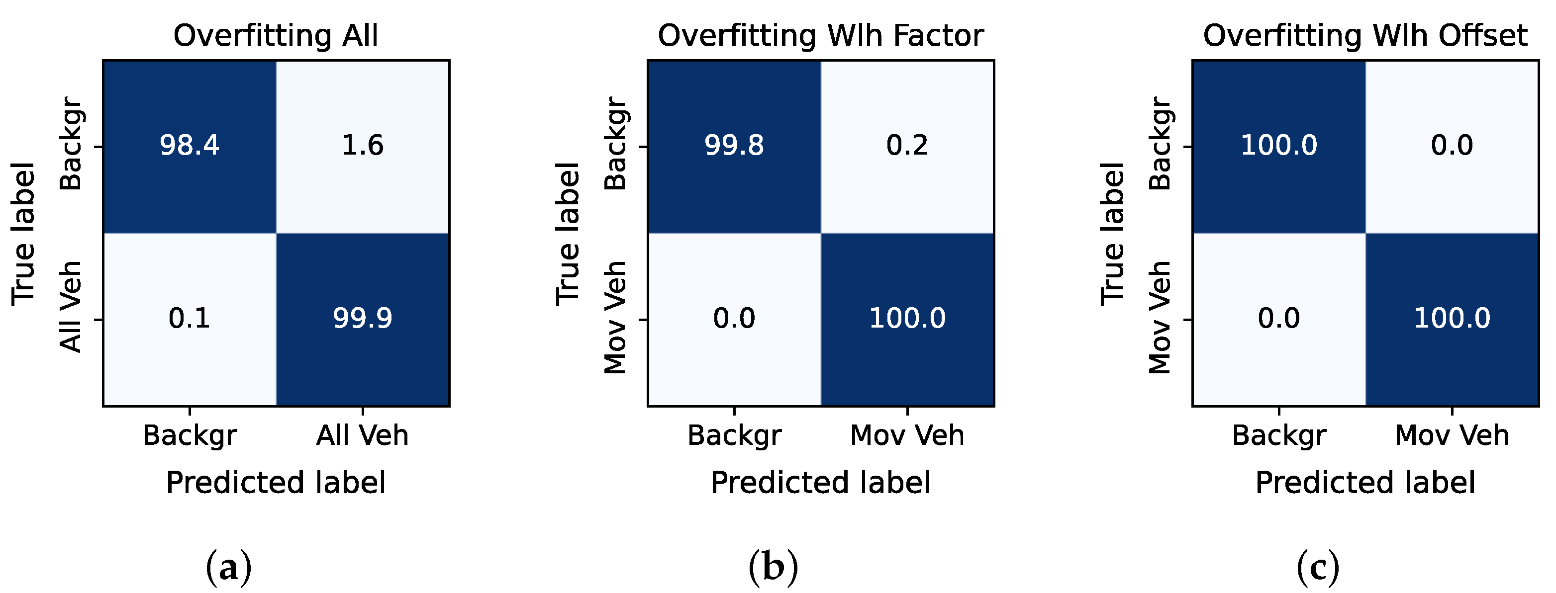
5.1. Model Critique
5.2. Data
6. Conclusions and Outlook
Author Contributions
Funding
Conflicts of Interest
References
- Geiger, A.; Lenz, P.; Stiller, C.; Urtasun, R. Vision meets Robotics: The KITTI Dataset. Int. J. Robot. Res. 2013, 32, 1231–1237. [Google Scholar] [CrossRef]
- Caesar, H.; Bankiti, V.; Lang, A.H.; Vora, S.; Liong, V.E.; Xu, Q.; Krishnan, A.; Pan, Y.; Baldan, G.; Beijbom, O. nuScenes: A multimodal dataset for autonomous driving. In Proceedings of the Conference on Computer Vision and Pattern Recognition (CVPR2020), Washington, DC, USA, 16–18 June 2020. [Google Scholar]
- Yoneda, K.; Suganuma, N.; Yanase, R.; Aldibaja, M. Automated driving recognition technologies for adverse weather conditions. IATSS Res. 2019, 43, 253–262. [Google Scholar] [CrossRef]
- Wu, B.; Zhou, X.; Zhao, S.; Yue, X.; Keutzer, K. SqueezeSegV2: Improved Model Structure and Unsupervised Domain Adaptation for Road-Object Segmentation from a lidar Point Cloud. In Proceedings of the International Conference on Robotics and Automation (ICRA), Montreal, QC, Canada, 20–24 May 2019. [Google Scholar]
- Milioto, A.; Vizzo, I.; Behley, J.; Stachniss, C. RangeNet ++: Fast and Accurate lidar Semantic Segmentation. In Proceedings of the 2019 IEEE/RSJ International Conference on Intelligent Robots and Systems (IROS), Macau, China, 3–8 November 2019; IEEE: Piscataway, NJ, USA, 2019; pp. 4213–4220. [Google Scholar] [CrossRef]
- Qi, C.R.; Su, H.; Mo, K.; Guibas, L.J. PointNet: Deep Learning on Point Sets for 3D Classification and Segmentation. In Proceedings of the IEEE Conference on Computer Vision and Pattern Recognition, Honolulu, HI, USA, 21–26 July 2017. [Google Scholar]
- Qi, C.R.; Yi, L.; Su, H.; Guibas, L.J. PointNet++: Deep Hierarchical Feature Learning on Point Sets in a Metric Space. arXiv 2017, arXiv:1706.02413. [Google Scholar]
- Thomas, H.; Qi, C.R.; Deschaud, J.E.; Marcotegui, B.; Goulette, F.; Guibas, L.J. KPConv: Flexible and Deformable Convolution for Point Clouds. In Proceedings of the IEEE/CVF International Conference on Computer Vision (ICCV), Seoul, Korea, 27 October–2 November 2019. [Google Scholar]
- Liang, Z.; Zhang, M.; Zhang, Z.; Zhao, X.; Pu, S. RangeRCNN: Towards Fast and Accurate 3D Object Detection with Range Image Representation. arXiv 2020, arXiv:2009.00206. [Google Scholar]
- Shi, S.; Guo, C.; Jiang, L.; Wang, Z.; Shi, J.; Wang, X.; Li, H. PV-RCNN: Point-Voxel Feature Set Abstraction for 3D Object Detection. In Proceedings of the IEEE/CVF Conference on Computer Vision and Pattern Recognition (CVPR), Seattle, WA, USA, 14–19 June 2020. [Google Scholar]
- Zhou, Y.; Tuzel, O. VoxelNet: End-to-End Learning for Point Cloud Based 3D Object Detection. In Proceedings of the IEEE Conference on Computer Vision and Pattern Recognition, Salt Lake City, UT, USA, 18–22 June 2018. [Google Scholar]
- Yang, Z.; Sun, Y.; Liu, S.; Shen, X.; Jia, J. STD: Sparse-to-Dense 3D Object Detector for Point Cloud. In Proceedings of the IEEE/CVF International Conference on Computer Vision (ICCV), Seoul, Korea, 27 October–2 November 2019. [Google Scholar]
- Hochreiter, S.; Schmidhuber, J. Long short-term memory. Neur. Comput. 1997, 9, 1735–1780. [Google Scholar] [CrossRef] [PubMed]
- Finn, C.; Goodfellow, I.; Levine, S. Unsupervised Learning for Physical Interaction through Video Prediction. arXiv 2016, arXiv:1605.07157. [Google Scholar]
- Lu, Y.; Lu, C.; Tang, C.K. Online Video Object Detection Using Association LSTM. In Proceedings of the 2017 IEEE International Conference on Computer Vision (ICCV), Venice, Italy, 22–29 October 2017; pp. 2363–2371. [Google Scholar] [CrossRef]
- Fan, H.; Yang, Y. PointRNN: Point Recurrent Neural Network for Moving Point Cloud Processing. arXiv 2019, arXiv:1910.08287. [Google Scholar]
- Schumann, O.; Wohler, C.; Hahn, M.; Dickmann, J. Comparison of Random Forest and Long Short-Term Memory Network Performances in Classification Tasks Using Radar. In Proceedings of the 2017 Symposium on Sensor Data Fusion: Trends, Solutions, Applications (SDF), Bonn, Germany, 10–12 October 2017; IEEE: Piscataway, NJ, USA, 2017; pp. 1–6. [Google Scholar] [CrossRef]
- Ester, M.; Kriegel, H.P.; Sander, J.; Xu, X. A Density-Based Algorithm for Discovering Clusters in Large Spatial Databases with Noise. In Proceedings of the Second International Conference on Knowledge Discovery and Data Mining, Portland, OR, USA, 2–4 August 1996; pp. 226–231. [Google Scholar]
- Lombacher, J.; Hahn, M.; Dickmann, J.; Wohler, C. Potential of radar for static object classification using deep learning methods. In Proceedings of the 2016 IEEE MTT-S International Conference on Microwaves for Intelligent Mobility (ICMIM), San Diego, CA, USA, 19–20 May 2016; pp. 1–4. [Google Scholar] [CrossRef]
- Schumann, O.; Hahn, M.; Dickmann, J.; Wohler, C. Semantic Segmentation on Radar Point Clouds. In Proceedings of the 2018 21st International Conference on Information Fusion (FUSION), Cambridge, UK, 10–13 July 2018; IEEE: Piscataway, NJ, USA, 2018; pp. 2179–2186. [Google Scholar] [CrossRef]
- Schumann, O.; Lombacher, J.; Hahn, M.; Wohler, C.; Dickmann, J. Scene Understanding With Automotive Radar. IEEE Trans. Intell. Veh. 2020, 5, 188–203. [Google Scholar] [CrossRef]
- Palffy, A.; Dong, J.; Kooij, J.F.P.; Gavrila, D.M. CNN based Road User Detection using the 3D Radar Cube. IEEE Robot. Automat. Lett. 2020, 5, 1263–1270. [Google Scholar] [CrossRef]
- Danzer, A.; Griebel, T.; Bach, M.; Dietmayer, K. 2D Car Detection in Radar Data with PointNets. In Proceedings of the 2019 IEEE Intelligent Transportation Systems Conference (ITSC), Auckland, New Zealand, 27–30 October 2019. [Google Scholar]
- Chadwick, S.; Maddern, W.; Newman, P. Distant Vehicle Detection Using Radar and Vision. In Proceedings of the 2019 International Conference on Robotics and Automation (ICRA), Montreal, QC, Canada, 20–24 May 2019. [Google Scholar]
- Nobis, F.; Geisslinger, M.; Weber, M.; Betz, J.; Lienkamp, M. A Deep Learning-based Radar and Camera Sensor Fusion Architecture for Object Detection. In Proceedings of the Sensor Data Fusion: Trends, Solutions, Applications (SDF), Bonn, Germany, 15–17 October 2019; pp. 1–7. [Google Scholar] [CrossRef]
- Yang, B.; Guo, R.; Liang, M.; Casas, S.; Urtasun, R. RadarNet: Exploiting Radar for Robust Perception of Dynamic Objects. In Proceedings of the European Conference on Computer Vision, Glasgow, UK, 23–28 August 2020. [Google Scholar]
- Shi, X.; Chen, Z.; Wang, H.; Yeung, D.Y.; Wong, W.K.; Woo, W.C. Convolutional LSTM Network: A Machine Learning Approach for Precipitation Nowcasting. In Proceedings of the 28th International Conference on Neural Information Processing Systems, Montreal, QC, Canada, 7–12 December 2015. [Google Scholar]
- Fent, F. Machine Learning-Based Radar Point Cloud Segmentation. Master’s Thesis, Technische Universität München, Munich, Germany, 2020. [Google Scholar]
- Lin, T.Y.; Goyal, P.; Girshick, R.; He, K.; Dollár, P. Focal Loss for Dense Object Detection. In Proceedings of the IEEE International Conference on Computer Vision (ICCV), Venice, Italy, 22–29 October 2017. [Google Scholar]
- Feng, D.; Haase-Schuetz, C.; Rosenbaum, L.; Hertlein, H.; Duffhauss, F.; Glaser, C.; Wiesbeck, W.; Dietmayer, K. Deep Multi-modal Object Detection and Semantic Segmentation for Autonomous Driving: Datasets, Methods, and Challenges. IEEE Trans. Intell. Transp. Syst. 2021, 22, 1341–1360. [Google Scholar] [CrossRef]
- Meyer, M.; Kuschk, G. Automotive Radar Dataset for Deep Learning Based 3D Object Detection. In Proceedings of the 2019 16th European Radar Conference (EuRAD), Paris, France, 2–4 October 2019; pp. 129–132. [Google Scholar]
- Bijelic, M.; Gruber, T.; Mannan, F.; Kraus, F.; Ritter, W.; Dietmayer, K.; Heide, F. Seeing Through Fog Without Seeing Fog: Deep Multimodal Sensor Fusion in Unseen Adverse Weather. In Proceedings of the IEEE/CVF Conference on Computer Vision and Pattern Recognition (CVPR), Seattle, WA, USA, 13–19 June 2020. [Google Scholar]
- Scheiner, N.; Schumann, O.; Kraus, F.; Appenrodt, N.; Dickmann, J.; Sick, B. Off-the-shelf sensor vs. experimental radar—How much resolution is necessary in automotive radar classification? In Proceedings of the 2020 IEEE 23rd International Conference on Information Fusion (FUSION), Rustenburg, South Africa, 6–9 July 2020. [Google Scholar]
- Yamada, N.; Tanaka, Y.; Nishikawa, K. Radar cross section for pedestrian in 76GHz band. In Proceedings of the Microwave Conference, Paris, France, 4–6 October 2005; IEEE: Piscataway, NJ, USA, 2005; pp. 4–1018. [Google Scholar] [CrossRef]
- Yasugi, M.; Cao, Y.; Kobayashi, K.; Morita, T.; Kishigami, T.; Nakagawa, Y. 79GHz-band radar cross section measurement for pedestrian detection. In Proceedings of the Asia-Pacific Microwave Conference proceedings (APMC), Seoul, Korea, 5–8 November 2013; IEEE: Piscataway, NJ, USA, 2013; pp. 576–578. [Google Scholar] [CrossRef]


| Network | All Vehicle Data Set | Moving Vehicle Data Set |
|---|---|---|
| PointNet++ | 59.91% | 75.83% |
| KPConv | 59.88% | 74.68% |
| KPConv-LSTM | 59.69% | 75.81% |
| KPConv-CLSTM | 60.05% | 75.42% |
| KPLSTM | 57.89% | 75.34% |
| KPconv w/o vel | 52.36% | 52.15% |
Publisher’s Note: MDPI stays neutral with regard to jurisdictional claims in published maps and institutional affiliations. |
© 2021 by the authors. Licensee MDPI, Basel, Switzerland. This article is an open access article distributed under the terms and conditions of the Creative Commons Attribution (CC BY) license (http://creativecommons.org/licenses/by/4.0/).
Share and Cite
Nobis, F.; Fent, F.; Betz, J.; Lienkamp, M. Kernel Point Convolution LSTM Networks for Radar Point Cloud Segmentation. Appl. Sci. 2021, 11, 2599. https://doi.org/10.3390/app11062599
Nobis F, Fent F, Betz J, Lienkamp M. Kernel Point Convolution LSTM Networks for Radar Point Cloud Segmentation. Applied Sciences. 2021; 11(6):2599. https://doi.org/10.3390/app11062599
Chicago/Turabian StyleNobis, Felix, Felix Fent, Johannes Betz, and Markus Lienkamp. 2021. "Kernel Point Convolution LSTM Networks for Radar Point Cloud Segmentation" Applied Sciences 11, no. 6: 2599. https://doi.org/10.3390/app11062599
APA StyleNobis, F., Fent, F., Betz, J., & Lienkamp, M. (2021). Kernel Point Convolution LSTM Networks for Radar Point Cloud Segmentation. Applied Sciences, 11(6), 2599. https://doi.org/10.3390/app11062599