C-Legged Hexapod Robot Design Guidelines Based on Energy Analysis

Abstract

C-legged hexapod robots offer a balanced trade-off between the robust stability of wheeled robots and the increased-motion capabilities of legged robots, and therefore, are currently of great interest. This article investigates the impact of mass, leg radius, and angular velocity on the energy consumption of C-legged hexapod robots, in order to develop a set of design guidelines that maximize the robot’s performance. The kinematic model of a single C-leg system is obtained and used to determine the system’s energy consumption associated with gravitational potential energy (GPE) and kinetic energy (KE) variations. Both the kinematic model and energy model are validated in a custom-made test bench. Our results show that the kinematic model very accurately predicts the trajectory of the system in space, but due to the varying load experienced by the motor, the system lags compared to the model predictions. Furthermore, the energy model has been also validated experimentally and successfully predicts the motor consumption periods. Using the energy model, it has been concluded that the angular velocity of the leg and the leg radius have an exponential relationship with motor peak power demand—directly affecting the motor selection. On the other hand, the mass is inversely proportional to the robot efficiency, and therefore, must be kept as low as possible.

1. Introduction

In recent years, the development and investigation of a large variety of mobile robots used in a wide diverse set of applications have been enhanced by electronics cost reduction, increased microchips computational capabilities, and intelligent and flexible manufacturing [1]. Mobile robots can be classified by the environment in which they work: land (UGVs), air (UAVs), or underwater (AUVs) [2].

Land robots can be further classified by their locomotion, which can be wheeled, tracked, or legged. Wheeled robots have the ability to reach high speeds with low power consumption and can be guided by controlling few degrees of freedom, but their ability to overcome obstacles is limited [3]. For this reason, although wheeled robots are the most prominent, tracked and legged robots offer motion advantages over the former in unstructured environments [4,5]. It is important to recall that most parts of the earth and other planet’s surfaces are inaccessible to conventional wheeled robots, due to the uneven terrain and obstacles, and therefore, there is a need to develop new mobile robots with enhanced mobile capacities. These natural terrains, on the other hand, offer a great opportunity for legged robots to demonstrate their terrain adapting capabilities [6]. The increased obstacle overcoming capabilities of legged robots can be explained by the fact that this type of robot does not require a continuous support surface, but uses a discrete foothold for each foot, enhancing their mobility [7].

On the other hand, the speeds achieved by legged robots are much lower, and energetically this type of robot is very inefficient. This is an important drawback in modern robotics as the battery energy-storing capabilities, and their heavy weight is a limiting design criterion [7]. Thus, it is critical for robots to be energy-efficient to maximize battery performance. Moreover, generally speaking, legged, robots have more actuators, making them difficult to build and demand complex control algorithms.

Legged robots are biologically inspired, and their design tries to replicate the walking motion of animals in nature: One leg robots are inspired by kangaroos, two-legged robots by bipeds, four legs on quadrupeds, and more than four legs are inspired by insects. The number of legs might be an evident classification criterion, but it is important to realize that the number of legs will also determine the gait stability, which can be static or dynamic. Robots with static gaits are always balanced as the robot weight vector always remains within the polygon formed by the legs in touch with the ground [8]. As a general rule, the more legs, the more stable the robot will be, but this will give rise to slow, inefficient, and complex legged robots.

In this paper, a hexapod robot will be considered, more specifically a C-leg shape hexapod robot. Hexapod robots are one of the most statically stable legged robots, and possess great flexibility, while standing or moving [9]. This stability combined with a simple C-leg design with only one degree of freedom per leg, offers a balanced trade-off between the increased mobility capabilities of legged robots and the robustness and high speeds of conventional wheeled robots [10]. Figure 1 shows a C-legged hexapod robot designed and manufactured by the Universidad Politécnica de Madrid.

Figure 1. C-Legged hexapod robot designed and Manufactured by the Centro de Automática y Robótica de la Universidad Politécnica de Madrid, picture taken by one of the article’s authors [11].

Figure 1. C-Legged hexapod robot designed and Manufactured by the Centro de Automática y Robótica de la Universidad Politécnica de Madrid, picture taken by one of the article’s authors [11].

One of the most well-known C-legged hexapod robots is RHex [12]. This project was funded by the Defense Advanced Research Projects Agency (DARPA) and involved many universities, such as the University of Michigan, McGill University, University of California, amongst others.

The synchronization possibilities of the six individual legs give rise to a variety of different gaits which determine the motion of the robot [13]. The two most common gaits are the alternating tripod gait mode and the six legs synchronized gait mode [10].

The alternating tripod gait mode is the standard walking/running gait used by Rhex. This gait groups the front and back leg from one side and the central leg from the opposite side to form two tripods. In this gait mode, one tripod is always in touch with the ground, while the other is moving freely in the air, offering increased speed and efficiency. A video simulation of this gait mode generated by implementing the kinematic model developed in this article in MATLAB can be seen in the Supplementary Materials.

The six legs synchronized gait mode, offers increased power and is generally used when hill climbing. On the other hand, this gait has reduced speed and reduced energy-efficiency, as at certain periods, the robot will lie on its chassis while the legs continue rotating. Similarly, to the alternating tripod gait, a video simulation of this gait mode can be seen in the Supplementary Materials.

Enhancing the energy-efficiency of legged robots has been a field of great interest and investigation in recent years [14]. These investigations have taken different routes, including (a) designing special robot structures that can reduce the energy consumption [15,16], (b) optimizing gait modes [13,17,18] (c) optimizing foot contact force [14], and (d) energy-efficient trajectory planning [19]. From these four different routes, the majority of the investigations have focused their efforts on optimizing the contact force to increase the robot’s efficiency. This type of optimization is based on the fact that over constraints of hexapod robots produce internal forces between contract points that ultimately lead to energy inefficiency and gait instability [14,20]. Implementing force distribution together with position control algorithms, ensures that adequate torque is applied at each joint reducing the energy wasted in each joint. On the other hand, the main objective of gait optimization is to increase the robots’ mobility performance [21], but it has also been proved that optimizing and switching between the different gait modes can save up to 20% [22]. Furthermore, switching between different gait modes can be combined with efficient trajectory planning, and information regarding the terrain can then be used to adequately choose between different gait modes [19].

All of the four optimization techniques have in common the fact that these investigations start with a robot design and their objective is to increase its performance, but it is possible that the design they start with, is inefficient compared to other design possibilities. Therefore, determining and knowing how different design parameters affect the core efficiency of the system is essential to obtain the best design possible, prior to the incorporation of all the different optimizations mentioned above.

Given the fact, that many of these investigations start with a design that needs optimization, the energy models are obtained by analyzing the energy consumption of each motor joint using the torque and the angular velocity [14]. In this article, the energy model will be obtained from a more macroscopic perspective and will be understood as the gravitational potential energy (GPE) and kinetic energy (KE) of the robot, allowing a generic hexapod robot to be considered. This offers a novel procedure to obtain the consumption of hexapod robots.

The objective of this article is to provide the reader with an understanding of the motion and energy consumption of hexapod robots, together with some design considerations, that will allow energy-efficient C-legged hexapod robots to be developed. To do so, the kinematic model and the energy model of a single C-leg system will be developed to determine the impact of mass, leg radius, and leg’s angular velocity on the energy consumption of the system. Even though a single C-leg system might seem physically far off from the actual robot, the reality is that the models developed in this article can be used to model a complete robot when moving under different gait modes. In fact, the equations obtained in this article for a single C-leg system also model the motion of a C-legged hexapod robot moving with all the legs synchronized. This is because in this gait mode, the six legs can be represented by a unique virtual leg. Moreover, the six legs in alternating tripod gait can be thought of as two virtual legs, and hence the robot’s motion is easily modeled using two individual C-leg models and synchronizing them out of phase. Videos of these two gait modes can be found in the Supplementary Materials.

The article is structured in the following way, firstly, the kinematic model of a single C-leg system is developed, which will be used to quantify the KE and GPE variations of the system, and therefore, the energy consumption and power demand associated with these variations. Then the kinematic and energy models will be validated experimentally on a custom-made test bench. Finally, the models will be used to investigate the impact of different design parameters on energy consumption, and a set of design guidelines will be drawn.

Finally, it is worthwhile mentioning that the models developed are not only useful to increase the efficiency of the system in terms of physical design, as well as in terms of gait motion. In fact, in continuation to the work presented in this article, the models presented here have been used to perform a gait optimization using an evolutionary algorithm.

2. Kinematic and Energy Model of a Single C-Leg System

2.1. Motion Mechanics

Let us start by considering a simplified system like the one shown in Figure 2, consisting of a square chassis represented in black and a semicircle leg (blue). The leg’s rotating point or hip (position where the motor is connected to the leg, represented in green) will be placed at the chassis center. The red dot will represent the contact point between the robot’s leg and the ground (black dotted line). The X-axis is the horizontal axis and is parallel to the ground and indicates the direction of forward and backward motion. The Y-axis is perpendicular to the ground line and is the direction in which gravity acts upon.

As the motor rotates in the anticlockwise direction, from an initial position shown in Figure 2, the system starts pivoting around the contact point (red dot in Figure 2), generating a circular trajectory with a radius equal to the legs diameter. This corresponds to the red trajectory that is shown in Figure 3 (left image). The angle rotated by the motor starting from the initial position (Figure 2) will be denoted $\theta$ and can be seen in Figure 3 (right image).

In the case of a dimensionless chassis, this pivoting type of motion continues until the hip touches the ground, configuration 2 in Figure 3 (right image). From this point and for the next $\frac{\pi }{2}$ radians the leg is rotating free, and thus, not moving the system.

When $\theta$ takes a value between $\pi$ and 2$\pi$, the leg gets back in touch with the ground, and the system starts moving again, but following a different trajectory than during the first period.

The leg’s orientation, in the limits of these intervals, can be seen in Figure 3 in the image on the right. Therefore, as it has been seen, the motion of the system can be split in to three different intervals in terms of the angle rotated by the motor $\theta$:

• $\theta \in \left[0,\frac{\pi }{2}\right]$: The system is pivoting around the contact point (Type I motion). It is important to note that this pivoting type of motion requires relatively slow rpms. Large rpm speeds will lead to the system to free fall, as the leg would be moving up in the vertical direction quicker than the chassis down. Hence, there would be no reaction force on the pivot point and no forward motion.
• $\theta \in \left[\frac{\pi }{2},\pi \right]$: The system is stationary.
• $\theta \in \left[\pi ,2\pi \right]$: The system is moving in a rolling type of motion (Type II motion).

In the model, developed in the following subsection, the following assumptions have been assumed:

• Massless leg: This is an acceptable assumption as it is important to note that the C-leg mass of hexapod robots accounts for only 5% of the total robot mass [10]. Therefore, assuming a massless leg will not largely impact the motion mechanics of the system and will still allow us to develop an adequate energy and power consumption model.
• Rigid one-dimension semi-circle leg: Compliant legs are an important feature in this kind of robot, as they enhance the robots’ mobility by deforming the legs shape according to the load experienced, and thus, acting as a suspension [23]. Even so, the compliant legs do not affect the fundamental motion behavior of the system. This means that a C-shaped leg will lead to a pivoting and cycloid motion of the system (as it will later be seen) no matter whether the leg is compliant or not. Having said this, the exact motion and position of the robot will be affected by the deformation experienced by the leg. In the analysis presented in this article, the aim is to analyze the core motion of these robots, to develop a model that can be used as a building block from which to build upon.
• No slip: Between the ground and the leg contact surface.

2.2. Kinematic Model

Firstly, let us start by placing the robot’s hip at the origin (0, 0), as shown in Figure 4. This means that the ground line (in this initial position) is located below the hip at twice the leg radius. This has been done to perform rotation matrix operations. Later in the kinematic model development, a vertical translation will be performed to set the ground to be the origin. In this way, the motion of the robot with respect to the floor will be determined.

As the shape of the leg is a semi-circle and the center coordinates are (0, −r) (Figure 4), its points can be parametrized in terms of the angle $\alpha$ in the following form:

$$x=rcos\left(\alpha \right)$$

(1)

$$y=rsin\left(\alpha \right)-\mathrm{r}$$

(2)

where $\alpha \in \left[\frac{-\pi }{2},\frac{\pi }{2}\right]$

Equations (1) and (2) represent the robot’s leg at the position, shown in Figure 4, but the objective is to obtain the leg’s position as it rotates. As previously stated, initially, the system’s hip is situated at (0, 0); therefore, the new legs position when rotated can be calculated by applying a 2D rotation matrix to the legs position equation.

That is, if (x, y) is a position of a point in the leg prior to a rotation, the position is given by:

$$\left[\begin{array}{c}{x}_{new}\\ y_{new}\end{array}\right]=\left[\begin{array}{cc}\cos \left(\theta \right)& -\sin \left(\theta \right)\\ \sin \left(\theta \right)& \cos \left(\theta \right)\end{array}\right]\left[\begin{array}{c}x\\ y\end{array}\right]$$

(3)

where $\theta$ is the angle of rotation around (0,0), with anticlockwise rotations being positive.

To determine the leg’s kinematic model, the contact point position with respect to the hip will be first identified. This can be done by finding the minimum in the expression for $y_{new}$ given in Equation (3).

$$\frac{d{y}_{new}}{d\alpha }=\cos \left(\alpha +\theta \right)=0$$

(4)

The solutions to Equation (1) will be denoted by ${\alpha }_e$; thus:

$${\alpha }_e=\frac{n\pi }{2}-\theta ,n=0,1.$$

(5)

For any leg rotation, there are two solutions, one corresponding to a maximum and another one to a minimum.

If $\frac{d^2{y}_{new}}{d{\alpha }^2}\left({\alpha }_e\right)<0$ then $y_{new}$ takes a maximum at ${\alpha }_e$, in this case ${\alpha }_e$ will be denoted as ${\alpha }_{max}$ and similarly if $\frac{d^2{y}_{new}}{d{\alpha }^2}>0$ $y_{new}$ is a minimum and will be denoted as ${\alpha }_{min}$.

Once ${\alpha }_{min}$ has been determined, the value needs to satisfy the condition of $\alpha \in \left[\frac{-\pi }{2},\frac{\pi }{2}\right]$ which has been previously established. If ${\alpha }_{min}$ lies within this range, then the solution identified belongs to the semicircle specified in the first part of the model. If it lies outside this range, then the minimum lies on the other symmetric semicircle, and the actual contact point corresponds to one of the range limits either $\frac{-\pi }{2}\mathrm{or}\frac{\pi }{2}$. Figure 5 shows a solution ${\alpha }_{min}$ outside the established interval mentioned above, and therefore, belongs to the symmetric semicircle.

Following the procedure described above, one can conclude that in a semicircle shaped leg the ${\alpha }_{min}$ angles corresponding to the contact point position are the following:

$${\alpha }_{min}=\left\{\begin{array}{c}\theta \in \left[0,\frac{\pi }{2}\right]\to {\alpha }_{min}=-\frac{\pi }{2}\\ \theta \in \left[\frac{\pi }{2},\pi \right]\to {\alpha }_{min}=\frac{\pi }{2}\\ \theta \in \left[\pi ,2\mathsf{\pi }\right]\to {\alpha }_{min}=\frac{n\pi }{2}-\theta ,n=0,1\end{array}\right.$$

(6)

Hence, combining the equations for the leg representation and the ${\alpha }_{min}$ values for each angle the contact position ($x_c,y_c)$ is given by:

$$\left[\begin{array}{c}{x}_c\\ y_c\end{array}\right]=\left[\begin{array}{cc}\cos \left(\theta \right)& -\sin \left(\theta \right)\\ \sin \left(\theta \right)& \cos \left(\theta \right)\end{array}\right]\left[\begin{array}{c}rcos\left({\alpha }_{min}\right)\\ rsin\left({\alpha }_{min}\right)-r\end{array}\right]$$

(7)

where ${\alpha }_{min}$ take the values specified in Equation (7) depending on the angle of rotation.

It is worthwhile noting that throughout one complete revolution, the ${\alpha }_{min}$ angles calculation are split into three separate intervals, which exactly coincide with the ones deduced in Motion Mechanics Section 2.1.

Up to this point, the equations for the contact point position have been determined with respect to the point of rotation and will now be used to determine the full trajectory of the system throughout one complete revolution. The hip coordinates of the system with respect to the initial position will be denoted by a subscript h. As mentioned in the Motion Mechanics subsection, and demonstrated when calculating the contact point position, the full legs revolution can be divided into three main intervals:

• $\theta \in \left[0,\frac{\pi }{2}\right]$: Where the system is pivoting around the contact point, Type I motion. Therefore, the global trajectory of the chassis is described with the following equation.

  $$\left[\begin{array}{c}{x}_h\\ y_h\end{array}\right]=\left[\begin{array}{c}{x}_c\\ -y_c\end{array}\right]=\left[\begin{array}{cc}\cos \left(\theta \right)& -\sin \left(\theta \right)\\ \sin \left(\theta \right)& \cos \left(\theta \right)\end{array}\right]\left[\begin{array}{c}rcos\left({\alpha }_{min}\right)\\ -rsin\left({\alpha }_{min}\right)+r\end{array}\right]$$

  (8)

  where ${\alpha }_{min}=-\frac{\pi }{2}$
• $\theta \in \left[\frac{\pi }{2},\pi \right]$: The system is stationary as the leg is not in touch with the ground, therefore, the x position of the system is the distance covered during the first interval:

  $$\left[\begin{array}{c}{x}_h\\ y_h\end{array}\right]=\left[\begin{array}{c}-2r\\ 0\end{array}\right]$$

  (9)
• $\theta \in \left[\pi ,2\pi \right]$: The system is rolling around the legs shape, Type II motion. In this type of motion, the trajectory is not only determined by the contact point position, but by the shape of the leg on which it is rolling. In the case of a semi-circle, the hips trajectory corresponds to a cycloid.

The goal is to obtain the position of Point H (the robot’s hip) as the leg rotates, with respect to an initial position corresponding to a rotation of $\theta =\pi$ (Point B).

The vertical coordinate of Point H is simply $-y_c$. On the other hand, the horizontal coordinates of Point H can be obtained using the following relationship between the horizontal components of the different points, shown in Figure 6:

$${\left(\overrightarrow{HB}\right)}_x={\left(\overrightarrow{AB}\right)}_x-{\left(\overrightarrow{AH}\right)}_x$$

(10)

${\left(\overrightarrow{AB}\right)}_x$ is given by $r\left(\frac{\pi }{2}-{\alpha }_{min}\right)$ assuming no slip, and ${\left(\overrightarrow{AH}\right)}_x$ is $x_c$. Therefore, the trajectory of the system when in Type II motion is given by:

$$\left[\begin{array}{c}{x}_h\\ y_h\end{array}\right]=\left[\begin{array}{c}r\left(\frac{\pi }{2}-{\alpha }_{min}\right)+x_c\\ -y_c\end{array}\right]$$

(11)

where $\left[\begin{array}{c}{x}_c\\ -y_c\end{array}\right]=\left[\begin{array}{cc}\cos \left(\theta \right)& -\sin \left(\theta \right)\\ \sin \left(\theta \right)& \cos \left(\theta \right)\end{array}\right]\left[\begin{array}{c}rcos\left({\alpha }_{min}\right)\\ -rsin\left({\alpha }_{min}\right)+r\end{array}\right]$ and ${\alpha }_{min}=\frac{n\pi }{2}-\theta ,n=0,1$.

According to the way the system motion is being developed, this rolling type of motion occurs after the pivoting motion. Therefore, the system has covered some distance prior to Type II motion. In the case of a dimensionless chassis this corresponds to 2r:

$$\left[\begin{array}{c}{x}_h\\ y_h\end{array}\right]=\left[\begin{array}{c}r\left(\frac{\pi }{2}-{\alpha }_{min}\right)+x_c+2r\\ -y_c\end{array}\right]$$

(12)

Equations (9), (10) and (13) express the motion of the system in terms of a rotation angle $\theta$ with respect to an initial position, but these equations can be expressed in terms of time:

$$\theta =\omega t$$

(13)

where $\omega$ is the angular velocity of the motor and t is the time elapsed since the initial position.

Therefore, the system’s position can be determined at any instant in time, and the speeds and accelerations can be obtained by deriving the equations.

The system has been considered to have a dimensionless chassis, and the Equations (9), (10) and (13) do not correspond to a real physical system. As it can be seen from the figure below, certain positions within the trajectory will imply the chassis to be below the ground.

The minimum height of the system’s hip, is actually determined by the distance between the bottom part of the chassis and the motor hip represented by $l_c$ in Figure 7. It is, therefore, important when implementing the model in code to perform the comparison between $y_h$ and $l_c$. If the system’s height is below the physical parameter, $l_c$ then that position does not exist, and the system is not moving.

2.3. Energy Model

2.3.1. Energy Consideration

Even in a simplified single C-legged system like the one being considered up to now in this article, there are many factors that contribute to the total energy consumption, and therefore, affect the power demand.

On the one hand, there are kinetic energy (KE) and gravitational potential energy (GPE) variations, which ultimately involve energy consumption and are dependent on the system’s kinematic model. It is worthwhile pointing out that this factor can be a big contributor to the total energy consumption, especially in legged robots, due to their complex kinematic motion, which produces non-linear trajectories. For example, a wheeled vehicle moving on a leveled, flat surface with the motors running at constant rpms will have no velocity changes, and therefore, no KE and no GPE changes. Let us now consider, a system consisting of a single C-leg shape moving on the same leveled, flat surface with the motor again set to constant rpms. In this case, the system will not be moving at a constant velocity or in a straight path, and therefore, will give rise to KE and GPE variations.

On the other hand, one can find the classic sources of energy consumption that appear in every moving system: Friction losses, elastic deformations, drag, motors internal resistance, etc.

In this subsection, the energy consumption and power demand, due to the motion of the system will be obtained using the Kinematic equations for a single C-Leg developed in the previous subsection. The Y- and X-directions will be considered separately. In the former, there are KE and GPE variations, while in the latter, only KE variations exist. Throughout this energy and power analysis, the system parameters that will be used for the graph representations will be a dimensionless system ($l_c=0$) with r = 0.2, m = 1 kg, $\omega$ = 60 rpm.

Afterwards, the total energy consumption and power demand will be calculated by adding the horizontal and vertical contributors, and the impact of the mass, and the leg radius and leg angular speed on the energy and power will be graphically analyzed.

2.3.2. Y-Axis (GPE and Power Demand Associated with GPE Variations)

The GPE of the system at any instant in time or angle of rotation is directly proportional to the height of the system $y_h$. As seen in the previous subsection and in Figure 8, the system’s height changes from a height of 2r to 0 in the case of a dimensionless chassis. Therefore, the GPE of the system at any moment in of rotation is given by:

$$GPE=mg{y}_h$$

(14)

The GPE of the system is not constant throughout a complete revolution, thus energy has to be removed and/or added to the system to follow the trajectory. The power demand to the motor, due to this GPE variation can be now calculated in the following form:

$$PowerdemanddueGPEvariations=\frac{dGPE}{dt}=mg\frac{d{y}_h}{dt}$$

(15)

From Equation (16), it can be observed that the power consumption is largely dependent on the speed of change of $y_h$ (velocity in the Y-axis).

The system’s hip height varies from 2r to 0 to back to 2r, this implies that there are positive and negative vertical velocities, shown in red in Figure 8.

Moreover, due to the lack of symmetry throughout a whole revolution, the system’s Y-axis velocity does not follow a smooth curve. A much rapid velocity can be seen in the first 0.25 s (corresponding to the Type I motion $\theta \in \left[\frac{\mathsf{\pi }}{2},\pi \right]$) compared to the Type II of motion. This is because in Type I motion, the system needs $\frac{\mathsf{\pi }}{2}$ radians to cover a distance of 2r, while in the second type of motion, the system has π radians to cover the same distance. When t = 0.25 s, the velocity drops to 0 m/s at this instant in time the robot’s hip hits the ground, and the leg is no longer in contact with the ground.

The power curve associated with the varying height is simply the rate of speed of change of height multiplied by the mass and the gravity, and therefore, only performs a scale transform on the curve.

Negative power values (as can be seen during the first 0.25 s in the right graph of Figure 8) imply that energy must be removed from the system. Therefore, during Type I motion, the system’s GPE is decreasing and needs to dissipate energy. On the other hand, in Type II motion, the system is gaining GPE, and therefore, this energy must be supplied, leading to positive power values (as can be seen in the last 0.5 s in the right graph in Figure 8).

2.3.3. Y-Axis (KE and Power Demand Associated with KE Variations)

The vertical component of the system’s velocity is not constant throughout one revolution, hence this leads to a power demand, due to KE variations in the Y-axis direction. The KE in this direction is given by:

$$K{E}_y=\frac{m}{2}{\left(\frac{d{y}_h}{dt}\right)}^2$$

(16)

In Figure 9, the $K{E}_y$ curve is shown, which is essentially the $\frac{d{y}_h}{dt}$ curve squared. To estimate the power demand associated with the KE energy variation of the system, the KE must be derived with respect to time.

$$P_{K{E}_y}=\frac{dK{E}_y}{dt}=m\frac{d^2{y}_h}{d{t}^2}\frac{d{y}_h}{dt}$$

(17)

Positive regions imply that the system needs to be supplied with energy in order for KE to increase, whilst in negative regions energy has to be removed from the system so to decrease the KE.

2.3.4. X-Axis (KE and Power Demand Associated with KE Variations)

Taking a look now at the X-axis, the only source of energy consumption is the KE in this direction which can be determined:

$$K{E}_x=\frac{m}{2}{\left(\frac{d{x}_h}{dt}\right)}^2$$

(18)

This KE is largely dependent on the speed of change of $x_h$, velocity in X-axis direction (Figure 10). The horizontal component of the system’s velocity is always positive, contrary to the vertical component where the system is oscillating. The power consumption due to KE variation in the horizontal direction is:

$$P_{K{E}_x}=\frac{dK{E}_x}{dt}=m\frac{d^2{x}_h}{d{t}^2}\frac{d{x}_h}{dt}$$

(19)

2.3.5. System’s Energy and Power Consumption Model

To obtain the total energy consumption, and therefore, the total motor power demand associated with KE and GPE variations, Equations (16), (18) and (20) are simply summed together.

$$P_{total}=P_{PE}+P_{K{E}_y}+P_{K{E}_x}$$

(20)

Taking the example that has been used throughout this article, the total power demand, due to the kinematic motion of a single-leg is:

Figure 11 shows the total power demand of the system throughout a complete revolution. During type I motion (0–0.25 s), one can observe that the power demand associated with the KE variations cancel out, this behavior might seem unexpected, but it can be explained by the mechanics of this type of motion. Under this type of motion, the system is essentially pivoting around the contact point position and at a constant angular velocity. Therefore, if the magnitude of the hip’s linear velocity vector $\left(\Vert v\Vert =\sqrt{v_x{}^2+v_y{}^2}\right)$ is calculated, the value should be constant during this type of motion.

$$\Vert v\Vert =\sqrt{{\left(2r\omega cos\left(\omega t\right)\right)}^2+{\left(-2r\omega sin\left(\omega t\right)\right)}^2}=2r\omega$$

(21)

Indeed, the magnitude of the hip’s linear velocity during Type I motion is constant and proportional to the leg’s radius and to the angular velocity, but this is not the case for Type II motion where the system is essentially rolling.

While the system is moving at a constant velocity, the total KE (sum of the KE in the X- and Y-direction) will be constant. For this reason, there is no power demand associated with KE variations in Type I motion.

The fact that the systems KE is constant, makes the net power demand during Type I motion only be the rate of change of GPE, leading to a negative power demand. Contrary to an object in free fall, our system has to lose GPE, while keeping the same KE, this means that this energy has to be dissipated via de motor. This can give rise to problems, such as components like microcontrollers burning down, if precautions are not taken. To avoid the flow of current in the opposite direction, the use of diodes is recommended.

Unlike Type I motion, during Type II motion, the net power demand is positive as the system must rise in height and accelerate, requiring energy to be supplied to the system.

The total power demand is not only useful from an energetical analysis perspective, but it can be very useful to identify the right motor for the robot. From these graphs, the maximum power of the motor can be determined, as well as the torque required. The torque exerted by the motor can be calculated using the power and angular velocity, as they are related together by the following equation:

$$\tau =\frac{P}{\omega }$$

(22)

where P is the power of the motor, τ the torque exerted by the motor and ω the angular velocity.

Therefore, the motor specifications when related to power and torque can be determined from the system’s physical properties, such as the legs radius, the mass and $l_c$.

3. Model Experimental Validation

3.1. Set-Up

To validate the kinematic and energy model developed in the previous section, it was necessary to design a test bench that matched the model assumptions. This meant to restrict the degrees of freedom of the system to only translation motion in the X- and Y-direction. To do so, the following test bench has been designed in SolidWorks and manufactured using a 3D printer.

The test bench consists of two sets of rail pairs that allow motion in the X- and Y-direction and limit the motion and rotation in the remaining degrees of freedom. To facilitate movement in the X- and Y-direction, IGUS bearings have been fitted in the sliding parts.

The motor used throughout the set of experiments is the JGY-371 motor with the specifications seen in

Table 1. Motor specifications.

Motor Specifications
Max rpms	40
Nominal Torque	5.6 kg·cm
Max Torque	24 kg·cm
Gear Ratio	150
Encoder Counts	16 Counts/rev prior gear reduction

:

Due to the motor’s worm gearbox, the minimum distance between the shaft and the edge of the gearbox is 16 mm. This means that the system’s hip will never be at a height lower than 16 mm above the ground, thus the value of $l_c$ is 16 mm. The motor driver used is the MDD10A which controls the motor speed, which has been set either to 30 rpm in the open loop or to 30 rpm with the PID close loop control.

To validate the kinematic model, two distance sensors were used. On the one hand, the distance sensor used to measure the height (y) was an ultrasonic sensor (hc-sr04), placed in the vertical slider, shown in Figure 12. On the other hand, to measure the displacement in the X-axis, a ToF sensor (cj vl53l0xv2) was placed in between the horizontal rails, and it measures the distance between the slider and the rail’s end. The position of this sensor can be seen in Figure 12. Both sensors are connected to an Arduino Uno, which sends the data back to MATLAB via serial communication.

The legs diameter used for the kinematic model experiment are r = 20 mm for the space trajectory validation and r = 15 mm, trajectory vs. time validation.

The leg has been designed to fulfill the conditions imposed during the development of the model. As it can be seen from Figure 13, the motor shaft and the legs end form a semicircle, and to avoid sliding, the legs contact surface has been made rugged. Furthermore, the leg’s end has been designed as thin as possible to ensure the system pivots around one unique point when the values of $\theta$ belong to the interval $\left[0,\frac{\pi }{2}\right]$.

To validate the energy model, the leg radius was set to be r = 15 mm (the same as the one used in the kinematic model validation). The INA219 sensor was used to measure the power consumption of the system. This sensor communicates via I2C to the Arduino Uno, which itself sends the data to a MATLAB script in the computer via serial.

It is important to note that the energy model developed predicts the power consumption of the motor, due to the GPE and KE energy changes. This means that if the power consumption is measured directly when the system is moving, then the energy consumption associated with other sources, such as internal frictions, resistances, inertias, etc., will be included in those measurements. To obtain the consumption associated strictly with GPE and KE variations, the following procedure was done.

Firstly, the power consumption of the motor at a constant $\omega$ with no load (i.e., leg rotating elevated from the ground), was measured. In this way, the power consumption associated with overcome the internal frictions, resistance, inertias, etc., is quantified; the results are shown in the left graph of Figure 17. Then the power consumption was measured when moving the whole system at the same constant $\omega$. The power consumption load-free was deducted from the total consumption to obtain the consumption associated with the energy changes of the system. There will also be other sources of energy consumption included in this final amount, such as friction losses between test-bench bearings and the rails and between the leg and the ground, but those should be negligible compared to the energy variations of the system.

To summarize, the model parameters can be seen in

Table 2. Model parameter energy model validation.

Model Parameters
$\omega$	30 rpm
$l_c$	0.016 m
$m$	0.315 kg
r	15 mm

.

3.2. Results and Discussion

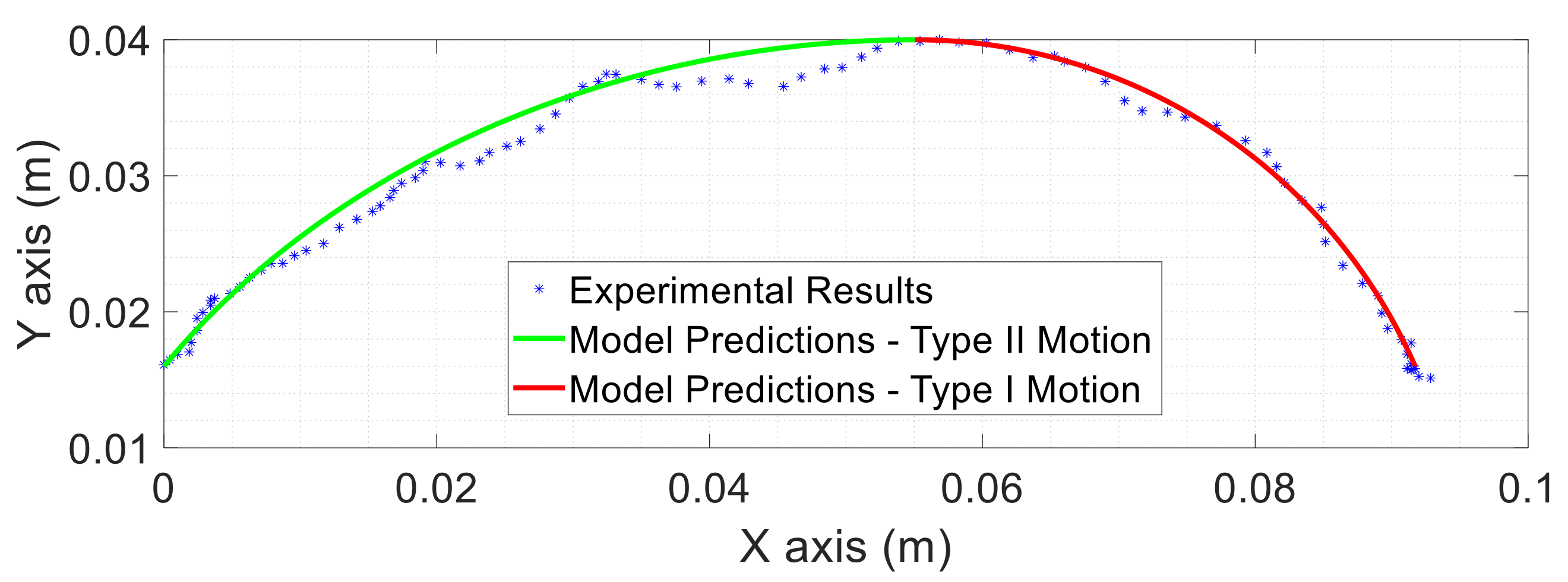
Overall, it can be seen that the experimental results accurately fit the model for both the trajectory in space (Figure 14) and the evolution of $x_h$ and $y_h$ in time (Figure 15).

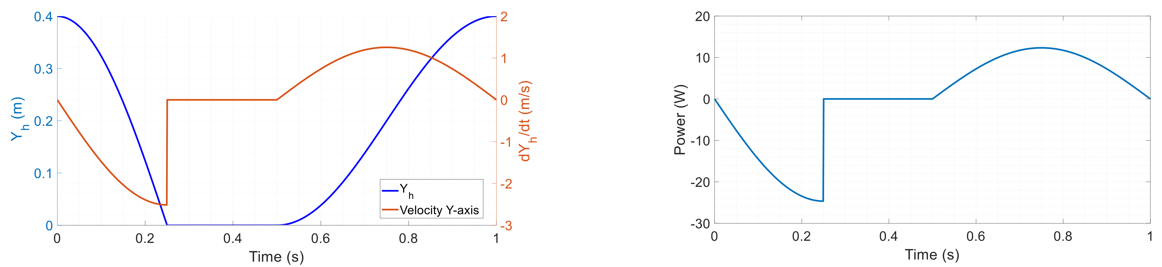
It can be seen that the system power demand to the motor is not constant throughout one entire revolution. Therefore, in an open loop control, the systems starts lagging as it can be seen in Figure 15. The motor changes from being rotating free of load, to having to rise the weight of system, to finally having to hold the weight of the system and avoiding it from free falling. These torque variation requirements can be accounted for using a close loop control—which, according to the error difference between the desired rpms and the actual rpms, changes the voltage input. Due to the non-linearity of the system, a PID control does not provide a suitable controller, as was noticed in the experiments.

Kinematic Model Validation: Trajectory

Figure 14. Motion Trajectory Experimental Results obtained with a system of r = 0.02 m throughout one complete revolution compared to the Model Predictions.

Figure 14. Motion Trajectory Experimental Results obtained with a system of r = 0.02 m throughout one complete revolution compared to the Model Predictions.

Kinematic Model Validation: Displacement evolution with time—2 cycles

Figure 15. Graphs showing the evolution of $y_h$ (left), and of $x_h$ (right) in time throughout two revolutions at 30 rpm in the open loop and in the close loop control, r = 0.015 m.

Figure 15. Graphs showing the evolution of $y_h$ (left), and of $x_h$ (right) in time throughout two revolutions at 30 rpm in the open loop and in the close loop control, r = 0.015 m.

In Figure 16, one can observe how the actual rpms of the system drop for both the open loop and close loop control, but on the close loop control the rpms overshoots straight after this decrease. This overshoot allows the system to catch up, and therefore, making it seem that at the end of the revolution, the system is not lagging Figure 15. In reality, the controller is not able to cope with the nonlinear load variation and is not capable of maintaining the 30 rpms. A more suitable controller, such as a fuzzy or adaptive controller, would allow for different responses at different rotation angles, which would allow for adequate control. Investigating a nonlinear controller for this application is very important for precise control, but is outside the scope of this article.

The legs dimensions were changed in the two experiments, because during the testing stage, it was noticed that a leg with r = 0.02 m required too much motor torque, which caused the system to lag even more. A reduced leg demands less torque, and therefore, allows the close loop control to be more reactive and meet the reference command sooner. On the other hand, a larger leg implies bigger changes in displacement, and for this reason, this size leg was left for the trajectory validation, shown in Figure 14.

Energy Model Validation:

The image on the left in Figure 17 shows the power consumption of the motor when no load is applied; this power consumption, as previously said, is due to internal resistance, friction losses, and inertial losses. It can be seen that the signal is noisy, but has a very constant average power consumption of 0.104 W. These oscillations could be due to many factors, such as oscillations in the supplying voltage, sensor errors, defects on the motor hardware, etc. It would be interesting to determine if there are some periodic variations associated with defects in the motor hardware that occur on every cycle. If this is the case, an average power consumption depending on the angular position of the motor, which would provide a more precise solution.

The image on the right in Figure 17 represents the motor’s power consumption when the system is moving, and therefore, a load is applied to the motor shaft. For most of the time, the motor consumption is constant and has the same value as the average power consumption measured when the motor had no load applied.

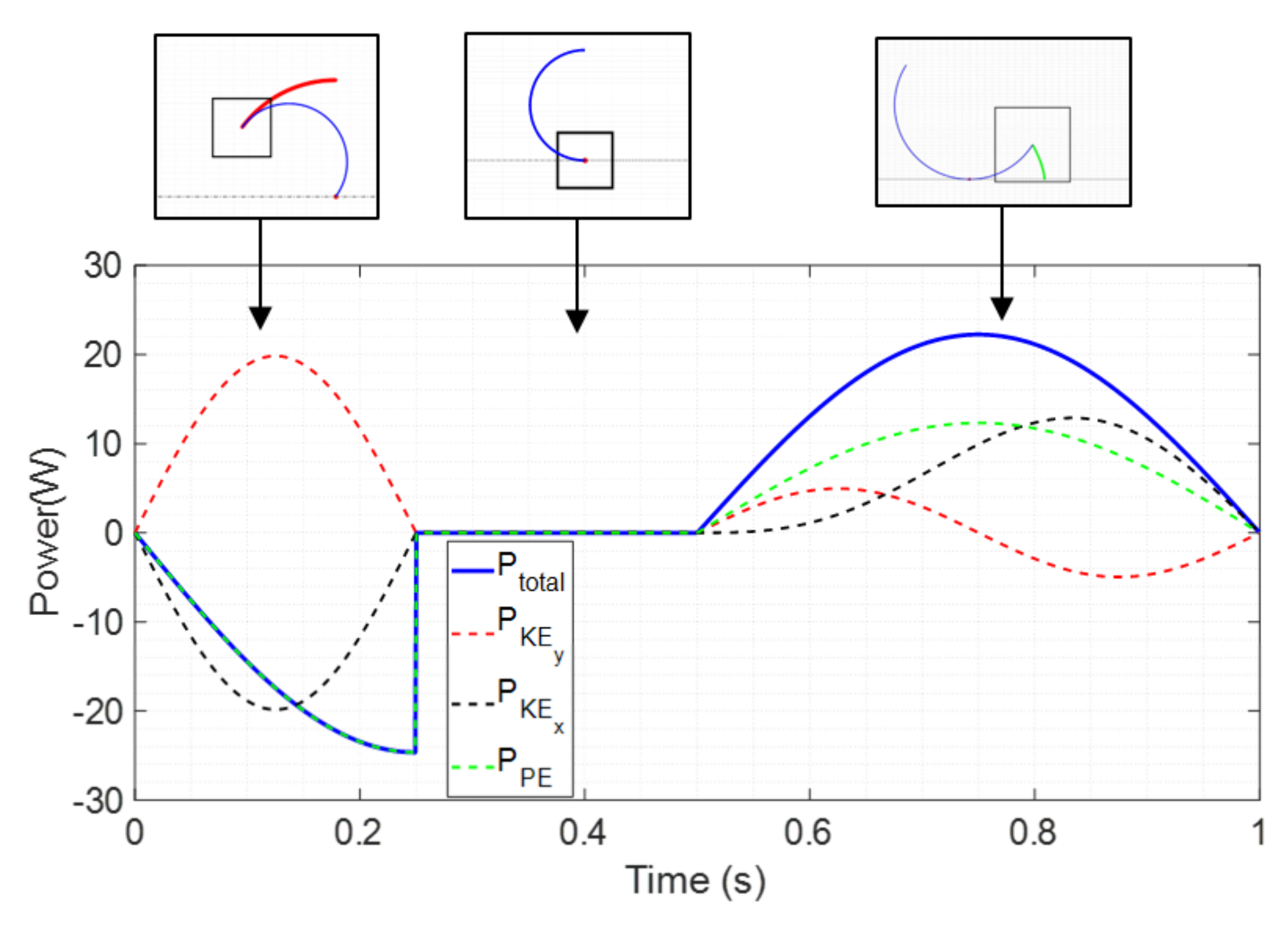
If the average power consumption under no load conditions is subtracted from the curve shown on the right image of Figure 17, the power consumption associated with the energy variations is obtained (Figure 18). This can be compared to the predictions obtained in the previous section (red line in Figure 18).

The predictions estimated a negative power demand during Type I motion as the system has to dissipate GPE, but this has not been detected by the sensors. After revisiting the equations and the equipment to explain this phenomenon, it was noticed that the motor used in the experiments contains a worm gearbox that self-locks to avoid the motor being back-driven [24]. In self-locking worm gears, the torque applied from the load side is blocked and will not drive the worm. This is ideal for applications where loading against the gravitational force is required, but this device will not allow for regenerative braking [25]. The energy applied is dissipated in heat, friction, and internal deflections. For this reason, the motor will drive, consuming the same power as if it was under no load conditions.

During Type II motion, it can be observed that the model predicts relatively accurately the power demand with an RMSE of 0.043. If the whole set of results are considered (Type I and Type II), then the RMSE increases to 0.077. As expected, the experimental values are higher than the predictions as friction losses between the leg and the ground have been neglected.

4. Design Parameters Impact on Power Demand and Energy Consumption

In this section, the effect $m,\omega$, and $r$ have on the power demand, and the energy consumption during a complete revolution will be analyzed. Instead of analyzing the energy consumption as a value in Joules, the horizontal distance ($x_h$) covered by the system with one Joule of energy will be considered instead. In this way, the efficiency in transforming energy to horizontal displacement can be determined and compared. No energy recovery will be assumed (similarly to the set-up used throughout the report); hence, negative power demands will be assumed to be 0, thus 0 energy consumed for these periods. Furthermore, the system will be considered dimensionless $l_c=0$.

4.1. Mass

The effect of the mass on power demand can be seen to be linear (left image in Figure 19). Although the relationship between the power demand and the mass is linear, this does not hold for the effect of mass on the distance covered with one joule. More mass implies more KE and more GPE variations, which leads to energy being wasted. From the right image in Figure 19, one can conclude that the relationship between the mass and the distance covered per joule is inversely proportional.

$$Distanceperjoule=\frac{1}{mass}$$

(23)

4.2. Angular Velocity

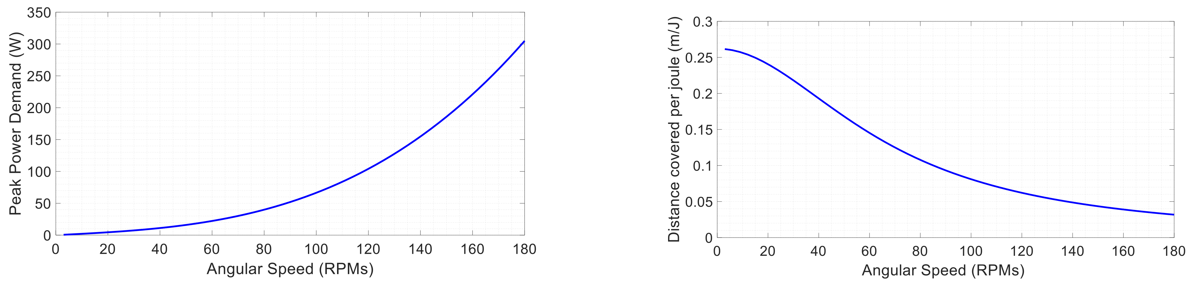
The effect of the angular velocity on the peak power demand can be seen not to be linear, but in fact, takes an exponential form (Figure 20). According to ^©Matlab’s regression toolbox, the exponential relationship, which has been determined using the nonlinear least squares method, has the following form [26]:

$$PeakPowerDemand=9.2e^{0.02\omega }$$

(24)

The confidence value returned by the toolbox for this regression fitting is 95%. Even though the exponential constant term is small (0.02), the impact of angular velocity on peak power demands is so large because of the wide range of possible angular velocities. Increased angular speeds imply that the leg’s rotation cycle time is reduced, meaning the energy variations need to be supplied quicker, leading to high peak power demands.

On the other hand, the angular velocity effect on the distance covered with one joule is not as drastic, as increased angular speeds only lead to higher KE variations (Figure 20). Whereas in the previous parameter analyzed (mass), increased mass implied increased KE and GPE hence its massive impact on the distance per joule.

4.3. Leg Radius

Larger legs require more instantaneous power demands (Figure 21), due to the systems increment in GPE and KE variations. The relationship between the leg’s radius and the peak power demand is not linear, but an exponential one. According to ^©Matlab’s regression toolbox, the exponential relationship has the following form:

$$PeakPowerDemand=8.5e^{0.5r}$$

(25)

The confidence value returned by the toolbox for this regression fitting is 95%. The exponential factor of this relationship (Figure 21, [26]) actually has a bigger value than the exponential growth rate seen between the angular velocity and the peak power demand (Figure 20, [25]).

Finally, the distance covered with 1 Joule of energy is inversely proportional to the leg’s radii (Figure 21).

4.4. Design Parameters Recommendations

The relationship obtained between the parameters analyzed and the peak power demand and the distance covered with one joule are sum up in the

Table 3. Angular velocity, mass, and leg radius effect on KE, GPE peak power demand and the distance covered per joule.

		KE		GPE		Peak Power Demand		Distance Covered per Joule
$\omega$		Lineal		IND		E. I		M.D
$m$		Lineal		Lineal		Lineal		I.P
$r$		Lineal		Lineal		Lineal		I.P
Small Impact	IND: Independent		Slight Impact		Lineal M.D: Moderate Decrease		Large Impact		E.I: Exponential Increase I.P: Inversely Proportional.

, the meaning of the different colors and acronyms are shown below this table.

Once again, it is worthwhile noting, that even though a simple C-leg system has been considered throughout the article, the conclusions obtained are the same as they would be for a full C-legged hexapod robot moving with all six legs synchronized. In an alternating tripod gait, the impact of the parameters investigated affects the energy and power consumption according to the synchronization of the two tripods, and can, therefore, be reduced.

With the conclusions obtained in the analysis performed in this section, the following recommendations are suggested to produce an efficient and well dimensioned C-legged hexapod robot. The following recommendations are for generic hexapod robots with no energy recovery, and therefore, no numbers that might be different for particular cases are used:

• Energy-Efficiency: To produce a robot efficient in the transformation of joules to distance covered, the mass has to be kept as low as possible. This is because the KE and GPE variations are increased, and that implies a greater loss of energy. For this reason, the mass reduction should be the main objective throughout the design stage.
• Motor Selection: Special care has to be taken when selecting the motors; as motors with high revolutions will need to supply really high-power demands. With the results obtained in Section 4, it is not recommended to have angular speeds over 140 rpms when the leg is in contact with the grounds, as higher rpms will lead to massive peak power demand, requiring the motor to be very powerful and to have high torque. Selecting a motor with so much power might also have the drawback of increased mass, which ultimately leads to a decrease in energy-efficiency. The 140 rpms recommendation when the leg is in contact with the ground does not imply the maximum rpms of the motor should be this. It is beneficial to have a motor with maximum rpms over this, so it can move quicker in rotation angles, where the power demand is low and then slower when the power demand is higher. This will allow for better gait synchronization, which can increase the efficiency of the system.
• Increasing Maximum Speed: If the maximum speed of the system wants to be increased, it might be worthwhile to increase the legs radius rather than selecting a motor with higher rpms. The desired maximum speed might be achieved with a larger leg that does not require a motor with so much power. On the other hand, this increase in leg radius will lead to more GPE and KE losses, but these losses will probably be smaller if this increase in leg radius has avoided choosing heavier motors. Moreover, the impact of the leg radius on the GPE and KE can be mitigated with gait synchronization.

As previously said, these recommendations are for hexapod robots with no energy recovery. If energy is recovered when the power demand is negative, then the relationship between the different variables changes slightly. It is important to remember that the negative power demand (during Type I motion) is associated with a decrease in GPE. In this period, energy has to be removed and is proportional to the mass and the height variation of the system. Hence, taking this into account and if energy recovery is implemented, then the impact of the system’s mass and leg radius on the distance covered with one joule, will be less than when there is no energy recovery. The energy-efficiency will be largely dependent on the ability to use the decrease in GPE. This could be by recharging the battery, which requires complex circuits, or using a supercapacitor that charges during those periods and releases the energy back to the motors during peak power demands. If the energy recovery efficiency is 100% then the mass and the leg radius will have no impact on the GPE, increasing the distance covered with one joule considerably. On the other hand, the impact of all the variables analyzed on peak power demand will be the same even if there is energy recovery.

5. Conclusions

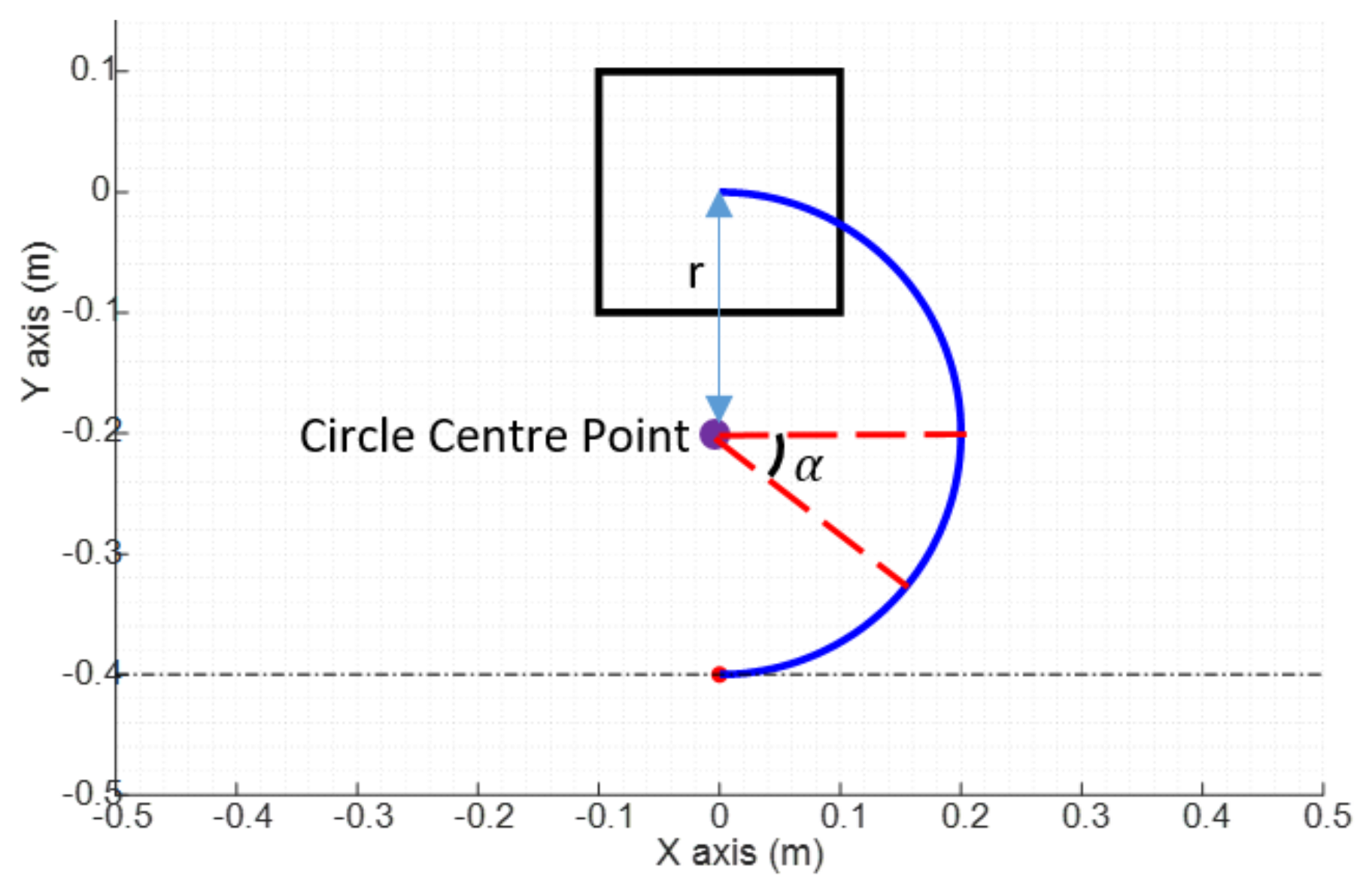
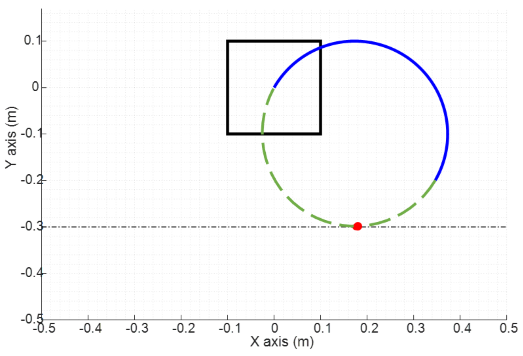
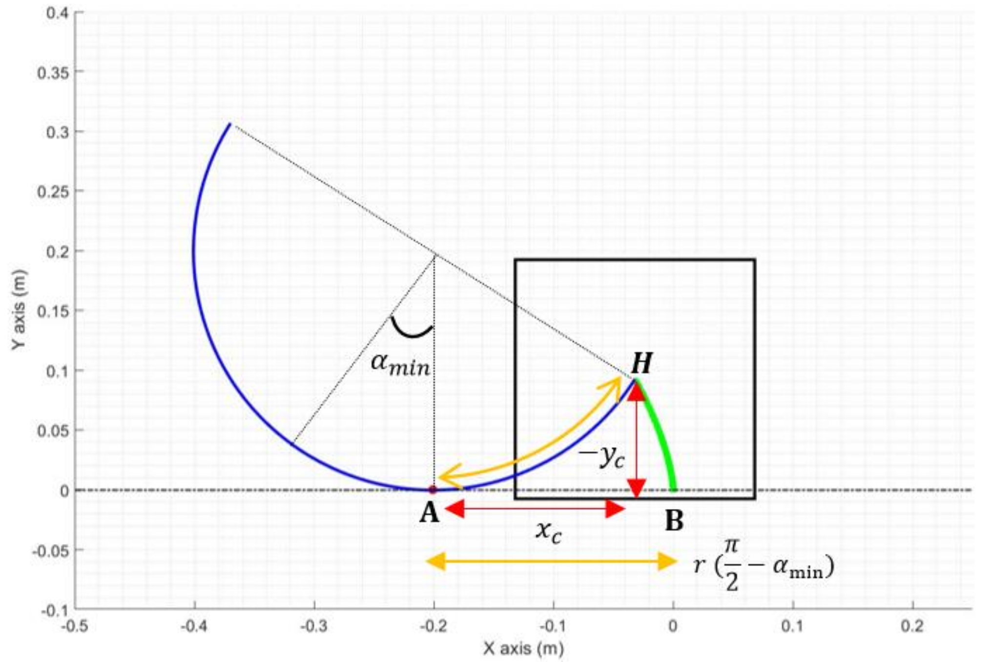
The kinematic model of a C-legged robot is the concatenation of two different types of motion, a pivoting and a rolling motion. This can be extended to other types of legs, such as ellipsoids. Based on the motion mechanics, a kinematic model has been developed for a semicircle shape leg. This model has been verified experimentally in a custom-made test bench, proving that the model predictions fit very accurately the motion of the system. During the experimental validation, it was noticed that the system tended to lag, and for this reason, a PID was implemented to maintain the revolution time constant. It would be later on discovered that the reason for this lag was the high-power demand required by the system to gain the GPE and KE in a short period of time. In fact, it was noticed that a PID could not cope with the nonlinearity of the system.

The procedure developed to obtain the kinematic model of the system has been made generic and can be easily extended to any leg form that can be parameterized by an angle $\alpha$. This means that the whole analysis performed in this article could be done for an ellipse or a C-leg shape leg bigger than a semicircle.

Building upon the kinematic model of a single-leg system, the KE and GPE of the system were determined and then used to obtain the power demand associated with this kinetic energy variation. The model predicts high peak power demands when the system has to rise, which caused the system to lag during the kinematic model validation. The energy and power demand was verified using the custom-engineered test bench and by measuring the power consumption of the motor. Due to the mechanics of the worm gearbox of the motor, only the positive power demand was able to be detected. During the periods of predicted negative power demands, the motor had no power consumption associated with the energy variations of the system.

Using the energy and power model, the impact of variables, such as the mass, the angular speed, and the leg radius, were investigated to draw a set of guidelines that help design and select motors for C-legged hexapod robot. It has been concluded that the mass of the system impacts drastically the efficiency of the robot, draining the battery capacity. Thus, the main objective in the design stage is to reduce the weight as much as possible, especially if no energy recovery method is implemented.

The angular speed of the leg has a large impact on the peak power demand as this variable reduces the time interval in which the energy has to be supplied. For this reason, it is recommended to keep the legs’ angular velocity when in contact with the ground to speeds below 140 rpms. Higher rpms require high-power demands, which might not be achieved by the motors. Selecting more powerful motors to achieve this power demand at high rpms, might lead to heavier motors, and therefore, a less efficient robot.

Moreover, the leg radius has an effect on the peak power demand and on the distance traveled with one joule, but its effect on these two evaluation parameters is smaller than the angular speed on the peak power demand and that of the mass on the energy-efficiency. Hence, it might be a good idea to increase the leg radius if the maximum speed of the robot wants to be increased.