Article

IpDFT-Tuned Estimation Algorithms for PMUs: Overview and Performance Comparison

1
Department of Industrial Engineering, University of Trento, 38123 Trento, Italy
2
Department of Measurements and Optical Electronics, Politehnica University of Timişoara, 300223 Timişoara, Romania
*
Author to whom correspondence should be addressed.
Appl. Sci. 2021, 11(5), 2318; https://doi.org/10.3390/app11052318
Submission received: 31 December 2020 / Revised: 17 February 2021 / Accepted: 26 February 2021 / Published: 5 March 2021
(This article belongs to the Special Issue Phasor Measurement Units: Algorithms, Challenges and Perspectives)

Abstract

:

Featured Application

Real-time measurement of amplitude, phase, frequency and rate of change of frequency (ROCOF) of current and voltage AC signals in power transmission and distribution systems.

Abstract

The Interpolated Discrete Fourier Transform (IpDFT) is one of the most popular algorithms for Phasor Measurement Units (PMUs), due to its quite low computational complexity and its good accuracy in various operating conditions. However, the basic IpDFT algorithm can be used also as a preliminary estimator of the amplitude, phase, frequency and rate of change of frequency of voltage or current AC waveforms at times synchronized to the Universal Coordinated Time (UTC). Indeed, another cascaded algorithm can be used to refine the waveform parameters estimation. In this context, the main novelty of this work is a fair and extensive performance comparison of three different state-of-the-art IpDFT-tuned estimation algorithms for PMUs. The three algorithms are: (i) the so-called corrected IpDFT (IpDFTc), which is conceived to compensate for the effect of both the image of the fundamental tone and second-order harmonic; (ii) a frequency-tuned version of the Taylor Weighted Least-Squares (TWLS) algorithm, and (iii) the frequency Down-Conversion and low-pass Filtering (DCF) technique described also in the IEEE/IEC Standard 60255-118-1:2018. The simulation results obtained in the P Class and M Class testing conditions specified in the same Standard show that the IpDFTc algorithm is generally preferable under the effect of steady-state disturbances. On the contrary, the tuned TWLS estimator is usually the best solution when dynamic changes of amplitude, phase or frequency occur. In transient conditions (i.e., under the effect of amplitude or phase steps), the IpDFTc and the tuned TWLS algorithms do not clearly outperform one another. The DCF approach generally returns the worst results. However, its actual performances heavily depend on the adopted low-pass filter.

1. Introduction

The Phasor Measurement Units (PMUs) are instruments designed to measure amplitude, phase, frequency, and Rate Of Change Of Frequency (ROCOF) of voltage and current AC signals in crucial locations of transmission and distribution systems [1]. While up to a few years ago PMUs were mainly conceived to detect anomalous operating conditions in transmission systems [2], nowadays they are regarded as essential devices to monitor the actual operating conditions of smart distribution grids in real-time, e.g., for island maneuvering [3], faulted line detection and identification [4], short-term voltage stability monitoring [5], and state estimation [6,7,8,9].
The key features of PMUs compared with other measurement devices for power system applications are:
  • the capability to measure all quantities at times synchronized with the Universal Coordinated Time (UTC);
  • the capability to stream real-time data to the so-called Phasor Data Concentrators (PDCs) with reporting rates ranging between about 10 frame/s and 100 frame/s;
  • high measurement accuracy, as specified in the IEEE/IEC Standard 60255-118-1:2018, in the following simply referred to as the “Standard” for the sake of brevity [10];
  • fast responsiveness (in the order of a few power line cycles) in order to trigger adequate protection schemes when severe phasor magnitude or phase changes occur due to faults or grid topology changes [11]. In this respect, the IEEE/IEC Standard classifies PMUs as protection-oriented (P Class) or measurement-oriented (M Class) devices. The former ones can indeed be less accurate than the latter, but of course they must be considerably faster.
Quite importantly, in the case of active distribution systems, the maximum Total Vector Error (TVE) of PMU measurements has to be even smaller than the Standard limits, i.e., in the order of 0.1% [12], and with phase uncertainty contributions not greater than a few mrad [13].
The need to meet the specifications shortly summarized above required remarkable research efforts in the area of signal processing and metrology. In particular, both flexible testbeds for PMU algorithm characterization [14], and new PMU calibrators were developed [15,16].
Among the many estimation algorithms for PMUs proposed over the last few years, the Interpolated Discrete Fourier Transform (IpDFT) is definitely one of the most popular, due to its low computational complexity and its good capability to compensate for the effect of off-nominal frequency deviations [17]. Such deviations might otherwise heavily affect the waveform parameter estimation based on the classic Discrete Fourier Transform (DFT) [18]. Even if the use of the IpDFT in signal processing is well established (e.g., for multi-tone parameter estimation [19]), its use in power systems monitoring applications was proposed only a few years ago. Since then, a number of IpDFT variants and multi-step algorithms based on the IpDFT stage have been developed to overcome the inherent limitation of the basic algorithm. In particular, the classic IpDFT algorithm can be used to obtain a preliminary estimate of some quantities of interest (most notably the fundamental frequency of the analyzed signal) prior to applying a further algorithm to return more accurate estimates of synchrophasor amplitude, phase, frequency, and ROCOF.
For instance, in [20], a three-point IpDFT algorithm is proposed to compensate for the infiltration of the spectral image of the fundamental component on the estimated parameters. However, this algorithm returns only a frequency estimate. This is indeed the most common case [21,22,23], although a dynamic ROCOF estimator based on IpDFT and Kalman filtering has been recently presented in [24]. The same idea also underlies the so-called enhanced IpDFT [25], which mitigates the detrimental effect of the image component on the estimated synchrophasor parameters by applying the IpDFT iteratively. In [26] this approach is further extended to compensate for the effect of harmonics and inter-harmonic components. The so-called corrected IpDFT (IpDFTc) consists of a two-step IpDFT designed to remove the spectral leakage due to both the image of the fundamental tone and the second-order harmonic [27]. In fact, these steady-state components are often the most critical ones for synchrophasor estimation, especially over short observation intervals. Quite importantly, the IpDFTc algorithm is not iterative. Therefore, it requires a lower computational burden than the estimator proposed in [26].
In [28] and [29] the fundamental frequency estimated through a classic IpDFT is used to tune the matrix coefficients of real-valued weighted least-squares estimators obtained from the Taylor’s series expansion of the dynamic synchrophasor model. In the original version of such estimators, the matrix coefficients are computed at the nominal frequency. As a consequence, the estimates are significantly affected by off-nominal frequency deviations. The IpDFT-based frequency tuning instead significantly improves the estimation accuracy of both the so-called Taylor-Fourier filter (which does not include the harmonics in the signal model) [30], and the Taylor-Fourier Transform (that instead includes a number of harmonics in the signal model) [31].
The preliminary fundamental frequency estimation based on the IpDFT can be also used to perform a better direct down-conversion of the voltage or current waveforms, before extracting synchrophasor amplitude and phase through low-pass filtering [32].
To the best of the Authors’ knowledge, the three IpDFT-tuned algorithms described above are among those that exhibit excellent performance in terms of both accuracy and computational complexity. Unfortunately, the results reported in the scientific literature do not allow a fair and easy comparison of their actual performances because different observation interval lengths or testing conditions are considered. Thus, this paper aims at presenting a thorough performance comparison of the IpDFTc estimator [27], the tuned Taylor Weighted Least Squares (TWLS) algorithm [28], and a tuned implementation of the frequency down-conversion and low-pass filtering (DCF) technique [32].
The rest of the paper is structured as follows. In Section 2, the theoretical background of the algorithms considered is briefly presented. In Section 3, the simulation results achieved in the steady-state, dynamic and transient testing conditions described in the IEEE/IEC Standard 60255-118-1:2018 are shown and commented on. Section 4 presents some final comments on the considered IpDFT-tuned algorithm compliance, advantages and disadvantages. Section 5 presents some further experimental results in borderline operating conditions compliant with the Standard EN 50160:2010 [33]. Finally, Section 6 concludes the paper.

2. Theoretical Background

In this Section, firstly a brief overview of the signal model used for synchrophasor, frequency, and ROCOF estimation is described. Then, the basic IpDFT algorithm used as a preliminary stage of all the techniques under test is recalled. Finally, the theoretical background of the three IpDFT-tuned estimators introduced in Section 1 is presented in a common framework.

2.1. Signal Model and Basic IpDFT Algorithm

Since the current or voltage AC waveform parameters change with time, a general AC waveform model is:
y ( t ) = s ( t ) + η ( t ) = a 1 ( t ) cos ( 2 π f 1 ( t ) t + ϕ 1 ( t ) ) + η ( t )
where s ( t ) = a 1 ( t ) cos ( 2 π f 1 t + ϕ 1 ( t ) ) is the fundamental sinewave (with amplitude, phase, and frequency at a given time t represented by a1(t), ϕ 1(t), and f1(t), respectively) and η(t) includes all possible disturbances, such as harmonics, inter-harmonics, and wideband noise. The sine-wave dynamic phasor is defined as p ( t ) = def a 1 ( t ) e j ϕ 1 ( t ) . It is called a synchrophasor when it is referred to timestamped UTC instants. If waveform (1) is sampled by a PMU at a rate fs and an odd number of samples M = 2Nh + 1 is acquired, the reference time tr for synchrophasor estimation (with r being integer) can be chosen exactly in the middle of the r-th digitized data record, which is given by:
y r ( m ) = a 1 ( r L + m ) cos ( 2 π f 1 ( r L + m ) f s ( r L + m ) + ϕ 1 ( r L + m ) ) + η ( r L + m )
for m = N h , , 0 , , N h , where L is the distance (in samples) between subsequent data records. Note that, in order to ensure a continuous data acquisition, L can range from 1 (if the observation intervals shift by 1 sample at a time) to M (when consecutive disjoint observation intervals are considered).
Thus, the objective of the estimation algorithms for PMUs is to determine the values of parameters a1(tr), ϕ1(tr) and f1(tr) and d f 1 ( t ) d t | t r at the chosen UTC reference time within the data record (2). Such data have to be transferred to the PDC at a given Reporting Rate RR. For this reason, in practice it is often reasonable to choose L = f s R R . In the following, the waveform parameters of interest within the r-th data record will be shortly denoted as a1,r, ϕ1,r f1,r and ROCOF1,r, respectively.
The ratio between the fundamental AC frequency f1,r and the sampling rate fs can be expressed as:
f 1 , r f s = ν 1 , r M = J 1 + δ 1 , r M ,
where ν1,r = J1 + δ1,r is the sinewave frequency expressed in bins, i.e., the number of acquired waveform cycles. Expression (3) results from the sum of an integer part J1 and a fractional part δ1,r (with −0.5 ≤ δ1,r < 0.5). While J1 typically does not change from record to record, the value of δ1,r changes as a function of time due to frequency fluctuations, and becomes zero only if coherent sampling is performed. The sampling rate is selected so that the following condition is fulfilled:
f n f s = J 1 M 1 .
where fn is the nominal sinewave frequency (i.e., 50 Hz or 60 Hz). Notice that the value of J1 coincides also with the number of cycles acquired at the nominal frequency.
In practice, a sinewave is usually sampled non-coherently (i.e., δ1,r ≠ 0). Therefore, the discrete spectrum of the acquired signal is affected by the spectral leakage due to the finite duration of the considered observation interval. The Maximum Sidelobe Decay (MSD) windows are often employed to reduce the impact of leakage on the estimated parameters [34,35]. The expression of a generic MSD window is:
w ( m ) = 1 2 2 H 2 [ C 2 H 2 H 1 cos ( 2 π M m ) + 2 h = 1 H 1 C 2 H 2 H h 1 cos ( 2 π h M m ) ] ,   m = N h , , 0 , , N h
where H ≥ 2 is the number of window terms and C n q = n   ! ( n q )   !   q   ! . In particular, the 2-term MSD (or Hann) window will be used in this paper. Since the DFT of the r-th windowed data record is given by
Y r , w ( k ) = def m = N h N h y r ( m ) · w ( m ) e j 2 π M k m ,
the preliminary estimates of the sine-wave parameters ν1, a1, and ϕ1 returned by the IpDFT algorithm are based on the DFT sample Yr,w(J1) and the larger of its two adjacent spectral samples, i.e., Yr,w(J1 − 1) or Yr,w(J1 + 1). In particular, it can be shown that [17]:
ν ^ 10 , r = J 1 + δ ^ 10 , r
with
δ ^ 10 , r = ( H 1 + i ) α 1 , r H + i α 1 , r + 1
in which α 1 , r = | Y r , w ( J 1 + i ) | | Y r , w ( J 1 + i 1 ) | with i = 0 if |Yr,w(J1 − 1)| > |Yr,w(J1 + 1)| or i = 1 if |Yr,w(J1 − 1)| < |Yr,w(J1 + 1)| and
a ^ 10 , r = 2 | Y r , w ( J 1 ) | W ( δ ^ 10 , r ) , ϕ ^ 10 , r = a n g l e { Y r , w ( J 1 ) } .
Note that in the estimator a ^ 10 , r , the DTFT of the window sequence (5) for M >> 1 and |λ| << M, is given with high accuracy by [36]
W ( λ ) = def m = N h N h w ( m ) e j 2 π λ M m = M sin ( π λ ) 2 2 H 2 π λ ( 2 H 2 )   ! h = 1 H 1 ( h 2 λ 2 ) .
which is a real-valued function due to the window even symmetry.

2.2. IpDFTc Algorithm

The IpDFTc estimator improves the performance of the basic IpDFT algorithm as it greatly reduces the effect on the estimated parameters of the spectral leakage due to both the image of the fundamental component and the second-order harmonic [27]. In the IpDFTc algorithm, the estimator of the number of observed signal cycles at the reference time within the r-th collected record is:
ν ^ 1 , r = ν ^ 10 , r Δ c ν 1 , r ,
where ν ^ 10 , r is returned by (8) and the term Δ c ν 1 , r is given by [27]:
Δ c ν 1 , r = Δ c δ 1 , r = ( H + ( 1 ) i δ ^ 10 , r ) [ ( 1 ) i 2 ν ^ 10 , r 2 ν ^ 10 , r δ ^ 10 , r + ( 1 ) i + 1 H W ( 2 ν ^ 10 , r δ ^ 10 , r ) W ( δ ^ 10 , r ) cos ( 2 ϕ ^ 10 , r ) + ( 1 ) i ( ν ^ 20 , r ν ^ 10 , r ) ν ^ 20 , r ν ^ 10 , r + δ ^ 10 , r + ( 1 ) i H a ^ 20 , r a ^ 10 , r W ( ν ^ 20 , r ν ^ 10 , r + δ ^ 10 , r ) W ( δ ^ 10 , r ) cos ( ϕ ^ 20 , r ϕ ^ 10 , r ) ] .
In (12) the values of a ^ 10 , r , ϕ ^ 10 , r result from (9), namely from the preliminary IpDFT, whereas a ^ 20 , r and ϕ ^ 20 , r are the amplitude and the phase estimators of the possible second-order harmonic at the same reference time tr. Let y ˜ r ( · ) be the residual signal obtained from (2) after subtracting the fundamental sinewave reconstructed by using the IpDFT estimated parameters, i.e.,
y ˜ r ( m ) = y r ( m ) a ^ 10 , r cos ( 2 π ν ^ 10 , r M ( r L + m ) + ϕ ^ 10 , r ) , m = N h , , 0 , , N h .
If Y ˜ r , w ( · ) is the windowed DFT of (13) obtained using the H-term MSD window [i.e., y ˜ r , w ( m ) = y ˜ r ( m ) · w ( m ) ], the amplitude and phase estimators of the second-order harmonic are obtained by applying the IpDFT algorithm to (13), that is:
a ^ 20 , r = 2 | Y ˜ r , w ( J 2 ) | W ( δ ^ 20 , r ) , ϕ ^ 20 , r = a n g l e { Y ˜ r , w ( J 2 ) } .
In (14), J2 denotes the integer part of the number of second harmonic cycles, while δ ^ 20 , r = ( H 1 + i ) α 2 , r H + i α 2 , r + 1 is the corresponding off-nominal frequency deviation estimator expressed in bins. Note that in α 2 , r = | Y ˜ r , w ( J 2 + i ) | | Y ˜ r , w ( J 2 + i 1 ) | the index i is equal to 0 if | Y ˜ r , w ( J 2 1 ) | > | Y ˜ r , w ( J 2 + 1 ) | or it is equal to 1 if | Y ˜ r , w ( J 2 1 ) | < | Y ˜ r , w ( J 2 + 1 ) | . Therefore, the second harmonic frequency, expressed in bins, is given by ν ^ 20 , r = J 2 + δ ^ 20 , r . In order to compensate for the effect of the spectral leakage caused by both the fundamental image component and the second harmonic, the following expression is applied to estimate the sine-wave amplitude at time tr:
a ^ 1 , r = a ^ 10 c , r Δ c a 1 , r
where
  • a ^ 10 c , r = 2 | Y r , w ( J 1 ) | W ( δ ^ 10 , r Δ c δ 1 , r ) (with δ ^ 10 , r and Δ c δ 1 , r given by (8) and (12), respectively) is the amplitude estimator of the fundamental sinewave after compensating for the fundamental frequency estimation bias due to the second harmonic and
  • Δ c a 1 , r = a ^ 10 , r W ( 2 ν ^ 10 , r δ ^ 10 , r ) W ( δ ^ 10 , r ) cos ( 2 ϕ ^ 10 , r ) + a ^ 20 , r W ( ν ^ 20 , r ν ^ 10 , r + δ ^ 10 , r ) W ( δ ^ 10 , r ) cos ( ϕ ^ 20 , r ϕ ^ 10 , r ) is the amplitude correction term [27].
Similarly, the IpDTFc synchrophasor phase estimator at time tr is
ϕ ^ 1 , r = ϕ ^ 10 , r Δ c ϕ 1 , r ,
where Δ c ϕ 1 , r = W ( 2 ν ^ 10 , r δ ^ 10 , r ) W ( δ ^ 10 , r ) sin ( 2 ϕ ^ 10 , r ) + a ^ 20 , r a ^ 10 , r W ( ν ^ 20 , r ν ^ 10 , r + δ ^ 10 , r ) W ( δ ^ 10 , r ) sin ( ϕ ^ 20 , r ϕ ^ 10 , r ) and ϕ ^ 10 , r results from (10).
Finally, the fundamental frequencies and the ROCOF are estimated respectively as:
f ^ 1 , r = f n + f s M δ ^ 1 , r .
and
R O C O F 1 , r ^ = | f ^ 1 , r f ^ 1 , r 1 | · f s L ,
in which if f ^ 1 , r and f ^ 1 , r 1 are the fundamental frequency estimates in two subsequent data records and L/fs represents the time interval between the corresponding UTC reference times.
Summarizing, the steps of the IpDFTc estimation algorithm are orderly reported in Table 1.

2.3. Tuned Real-Valued TWLS Algorithm

The fundamental component of (1) can be rewritten as:
s ( t ) = a 1 ( t ) cos ( 2 π f 1 t + ϕ 1 ( t ) ) = c 1 ( t ) cos ( 2 π f 1 t ) s 1 ( t ) sin ( 2 π f 1 t ) ,
where c1(t) = a1(t) cos ϕ 1 ( t ) and s1(t) = a1(t) sin ϕ 1 ( t ) . To implement the real-valued TWLS algorithm [28], the two quadrature components c1(t) and s1(t) are approximated by their respective Taylor’s series about the reference time tr truncated to the K-th order term (K ≥ 2). As a result,
c 1 ( t ) c 1 ( t r ) + c 1 ( 1 ) ( t r ) Δ t + c 1 ( 2 ) ( t r ) 2 ! Δ t 2 + + c 1 ( K ) ( t r ) K ! Δ t K
and
s 1 ( t ) s 1 ( t r ) + s 1 ( 1 ) ( t r ) Δ t + s 1 ( 2 ) ( t r ) 2 ! Δ t 2 + + s 1 ( K ) ( t r ) K ! Δ t K
where Δt = ttr and c 1 ( k ) ( t r ) , s 1 ( k ) ( t r ) , k = 1, 2,…, K, are the k-th order derivatives of c1(t) and s1(t), respectively, evaluated at the time instant tr. The original Taylor-based weighted approach described in [30] assumes that the sinewave frequency coincides with the nominal one, i.e., f1 = fn in (19). However, possible off-nominal frequency deviations may significantly affect the accuracy of the estimation results. This is why a preliminary IpDFT-based fundamental frequency estimation is recommended in [29].
Let us consider the r-th data record collected in the observation interval [ r L N h f s , r L + N h f s ] centered at the reference time t r = r L f s . If (20) and (21) are replaced into (19) and the resulting expression is evaluated and equated to each sample of the data record, a linear system of M = 2Nh + 1 equations with 2K unknowns and coefficients c 1 ( t r ) = c 1 , r ( 0 ) ,   c 1 ( k ) ( t r ) = ( k !   f s k ) c 1 , r ( k ) ,   s 1 ( t r ) = s 1 , r ( 0 ) ,   s 1 ( k ) ( t r ) = ( k !   f s k ) s 1 , r ( k ) , for k = 1, 2, …, K, can be built. If the unknown variables are gathered into vector P r [ c 1 , r ( K ) c 1 , r ( 1 )   c 1 , r ( 0 ) s 1 , r ( 0 ) s 1 , r ( 1 ) s 1 , r ( K ) ] T and f ^ 10 , r = ν ^ 10 , r f s M [with ν ^ 10 , r being given by (7)] is used to estimate f1 in (19), the coefficients of the linear system can be arranged into a matrix VK,r whose elements are [28]
( v K , 1 ) l q = ( l N h ) K + 1 q cos ( 2 π ν ^ 10 , r ( N h l ) ) , l = 1 , ,   N h , q = 1 , ,   K + 1 ( v K , 2 ) l q = l K + 1 q cos ( 2 π ν ^ 10 , r l ) , l = 1 , ,   N h , q = 1 , ,   K + 1 ( v K , 3 ) l q = ( l N h ) q 1 sin ( 2 π ν ^ 10 , r ( N h l ) ) , l = 1 , , N h , q = 1 , ,   K + 1 ( v K , 4 ) l q = l q 1 sin ( 2 π ν ^ 10 , r l ) , l = 1 , ,   N h , q = 1 , ,   K + 1
Thus, the weighted least squares approach returns the following estimate of vector P r :
P r ^ = ( V K , r T W T W V K , r ) 1 V K , r T W T W y r
where yr represents the column vector including the samples of the r-th data record (2) and W is a M × M diagonal matrix. The nonzero elements of W are the coefficients of the window function w(·) that is used to smooth the approximation error near the ends of each observation interval. It is worth recalling that if K = 2 the coefficients of P r ^ can be estimated not only in the time domain, but also in the frequency domain, as summarized in Appendix A. Due to the preliminary fundamental frequency tuning, the elements of V K , r have to be recomputed for every new record of collected data. For this reason, the complexity of the tuned-TWLS algorithm is generally greater than the computational burden of the IpDFTc estimator.
If the pairs of the real and the imaginary parts of the elements of vector P r ^ returned by (23) are combined into complex numbers (i.e., p ^ k , r = c ^ 1 , r ( k ) + j s ^ 1 , r ( k ) for k = 0 ,   1 ,   2 ), the synchrophasor magnitude and phase as well as the fundamental frequency and the ROCOF evaluated at time tr can be obtained respectively as
a ^ 1 = | p ^ 0 , r | , ϕ ^ 1 = a n g l e { p ^ 0 , r } ,
f ^ 1 , r = f n + f s 2 π I m { p ^ 1 , r p ^ 0 , r * } | p ^ 0 , r | 2   and
R O C O F ^ 1 , r = f s 2 π [ I m { p ^ 2 , r p ^ 0 , r * } | p ^ 0 , r | 2 R e { p ^ 1 , r p ^ 0 , r * } I m { p ^ 1 , r p ^ 0 , r * } | p ^ 0 , r | 4 ] .
Ultimately, the steps of the tuned real-valued TWLS estimation algorithm are orderly reported in Table 2.

2.4. Tuned Frequency Down-Conversion and Low-Pass Filtering (DCF)

As briefly outlined in the Introduction, the DCF approach is one of the most classic techniques for synchrophasor estimation. Indeed, it was mentioned in past editions of the Standard, too. The underlying idea is quite simple and it is very similar to the direct frequency down-conversion technique implemented in many radio receivers. If the samples of the r-th data record (2) are mixed with two digital quadrature sinewaves of unit amplitude and frequency f1,r, the following in-phase (I) and quadrature (Q) components of the input signal are obtained from the prosthaphaeresis formulas:
y r I ( m ) = y r ( m ) cos ( 2 π f 1 , r f s m ) = = a 1 ( r L + m ) 2 [ cos ( ϕ 1 ( r L + m ) ) + cos ( 4 π f 1 , r f s m + ϕ 1 ( r L + m ) ) ] + η I ( r L + m ) y r Q ( m ) = y r ( m ) sin ( 2 π f 1 , r f s m ) = = a 1 ( r L + m ) 2 [ sin ( ϕ 1 ( r L + m ) ) + sin ( 4 π f 1 , r f s m + ϕ 1 ( r L + m ) ) ] + η Q ( r L + m )
where η I ( · ) and η Q ( · ) are the contributions due to harmonics, inter-harmonics and wideband noise resulting from the frequency down-conversion of term η ( · ) in (2). Expression (27) shows clearly that, as a result of mixing, the power of the fundamental sinewave is evenly split into two components: one at DC, and another around 2f1,r. Similarly, every harmonic and inter-harmonic component is split into pairs of contributions shifted by ±f1,r with respect to their respective original frequency. It is worth emphasizing that the frequency of the digital quadrature oscillators can be hardly set exactly equal to the fundamental frequency f1,r. Therefore, in practice, either it is set equal to the nominal value fn (as suggested in the Standard) or it is extracted from the input signal. This can be done, for instance, by estimating f1,r with a phase-locked loop or with a preliminary IpDFT algorithm, as done in this paper [32].
Now, let h ( m ) be the impulse response of a digital low-pass filter with a a null phase response and with magnitude response | H ( e j ω ) | close to 2 in the passband (assuming a cutoff frequency ω < 2 π f n f s ), and to 0 in the stopband, respectively. If this filter is applied in parallel to both y r I ( m ) and y r Q ( m ) , it follows that
y ˜ r I ( m ) = y r I ( m ) h ( m ) = a 1 ( r L + m ) cos ( ϕ 1 ( r L + m ) ) + e r I ( m ) y ˜ r Q ( m ) = y r I ( m ) h ( m ) = a 1 ( r L + m ) sin ( ϕ 1 ( r L + m ) ) + e r Q ( m ) .
In (28) denotes the convolution operator, while e r I ( m ) and e r Q ( m ) are the error terms affecting the baseband I/Q components due to the filter non-idealities. These are due to (i) the frequency fluctuations of the quadrature sinewaves generated by the internal digital oscillator used for frequency down-conversion; (ii) the ripples affecting the gain of the low-pass filter in the passband; and (iii) the imperfect attenuation of both the double-frequency terms and all the disturbances lying in the stopband. However, if the filter is suitably designed, such error terms can be kept under control. Thus, from (28), it follows that synchrophasor magnitude and phase at time tr can be easily estimated as
a ^ 1 , r = | y ˜ r I ( m ) + j y ˜ r Q ( m ) | , ϕ ^ 1 , r = a t a n 2 ( y ˜ r Q ( m ) , y ˜ r I ( m ) )
where atan2(y,x) computes the principal value of the phase of a complex number x + jy between [−π, π]. Moreover, the sinewave fundamental frequency and its ROCOF can be estimated by applying the first-order and second-order backward Euler differences over subsequent data records, i.e.,
f ^ 1 , r = ( ϕ ^ 1 , r ϕ ^ 1 , r 1 ) f s 2 π L
and
R O C O F ^ 1 , r = f s 2 2 π L 2 ( ϕ ^ 1 , r 2 ϕ ^ 1 , r 1 + ϕ ^ 1 , r 2 ) .
Of course, the performances of the DCF approach strongly depend on the features of the adopted low-pass filter as well as on the accuracy of the frequency tuning of the sinewave used for down-conversion. In fact, if the signal nominal frequency fn rather than the estimated value of f1,r is used for down-conversion, the overall estimation accuracy can be heavily affected by possible off-nominal frequency deviations of the acquired signal, unless the filter passband is enlarged accordingly [37]. On the contrary, the frequency tracking of the fundamental component can be exploited to place the zeros of the filter frequency response at harmonic frequencies to mitigate their influence [32]. A custom approach to design optimal differentiator filters for PMUs is presented for instance in [38], but it is applied to the Taylor-Fourier Transform and not to the DCF method.
In the next Section, the results obtained with two alternative low-pass filters are reported. The steps of the tuned DCF estimation technique are instead summarized in Table 3.

3. Estimation Results and Performance Analysis

In this Section, the performances of the IpDFT-tuned algorithms presented in Section 2 are compared under multiple testing conditions. In particular, the maximum values of the following parameters are computed, i.e.,
  • the Total Vector Errors (TVEs), namely the magnitude of the error vectors of the estimated synchrophasor relative to the actual synchrophasor values at the same UTC reference times;
  • the Frequency Errors (FE), i.e., the differences between the estimated fundamental frequencies and the actual ones and
  • the Rate of change of Frequency Errors (RFEs) namely the differences between the estimated ROCOF values and the actual ones.
Such parameters are estimated assuming L = 120 and a reporting rate RR = 50 readings/s. This is the largest mandatory rate reported in the Standard [10]. To this purpose, the results of the IpDFT-tuned estimation algorithms under study are compared over 1000 data records in the P Class and M Class steady-state and dynamic testing conditions specified in [10]. The initial phase values of all possible disturbances (e.g., harmonics, inter-harmonics or modulating tones) are varied randomly with a uniform probability density function in the range [0, 2π]. Then, the TVE, |FE| and |RFE| response times as well as the corresponding delay times and the maximum overshoots due to amplitude or phase steps in the worst-case P Class and M Class simulated transient conditions reported in [10] are summarized. All the simulated P Class and M Class tests are performed assuming the following common settings, i.e., nominal fundamental frequency fn = 50 Hz, sampling frequency fs = 6 kHz and observation interval length ranging from J1 = 2 or 4 nominal power line cycles for P Class tests to J1 = 6 or 8 nominal power line cycles for M Class tests.
Such observation interval values were chosen as they provide a good trade-off between estimation accuracy and responsiveness, although with actual performances that may differ considerably from case to case. The preliminary IpDFT stage (common to all algorithms) is based on the 2-term MSD (or Hann) window defined in [35] with two DFT interpolation points [17]. Quite importantly, the TVE, |FE|, and |RFE| values achievable with the IpDFTc algorithm in steady-state tests with off-nominal frequency and harmonics are much lower than those obtained with the classic IpDFT estimator, as confirmed by Figure 1. In the other testing conditions instead, the results of the IpDFTc and the IpDFT almost coincide. Therefore, in the rest of this paper the latter ones are omitted for the sake of brevity. In Figure 1 the curves with different line styles and colors refer to the maximum TVE, |FE| and |RFE| values returned by the classic IpDFT and the IpDFTc estimators as a function of the off-nominal frequency deviation. Such maxima are computed over 1000 6-cycle-long or 8-cycle-long records, assuming that the first 50 harmonics (all of them with amplitude equal to 10% of the fundamental component) affect the collected waveform. The benefits of the compensation of the leakage due to both the second-order harmonic and the fundamental image component are evident (particularly in the 6-cycle case) and justify the adoption of the IpDFTc approach in the following analysis. Further results (not shown for the sake of brevity) confirm that the IpDFTc algorithm can meet the P Class limits reported in the Standard even over 3-cycle observation intervals, whereas the classic IpDFT estimator cannot.

3.1. P Class and M Class Steady-State and Dynamic Testing Conditions

The main P Class and M Class steady-state and dynamic testing conditions specified in [10] are briefly recalled below.
  • Fundamental frequency off-nominal static deviations within ±2 Hz (P Class) or ±5 Hz (M Class);
  • Harmonics from the 2nd to the 50th (taken one at a time) with amplitude set to 1% (P Class) or 10% (M Class) of the fundamental with the same off-nominal frequency deviations mentioned above;
  • Amplitude modulation (AM) or phase modulation (PM) with modulation indexes equal to ka = 0.1 or kp = 0.1 rad, respectively, and frequency of the modulating tones equal to fa = fp = 2 Hz (P Class) or 5 Hz (M Class);
  • Linear increment/decrement of the fundamental frequency at rates of ±1 Hz/s within ±2 Hz (P Class) or ±5 Hz (M Class);
  • White zero-mean Gaussian noise with variance such that the Signal-to-Noise Ratio (SNR) is 60 dB (this testing condition is not mentioned in the IEEE/IEC Standard, but it has a high practical relevance due to the strong impact of wideband noise on frequency and above all ROCOF estimation [39]);
  • Finally, in the M Class case only, a single inter-harmonic tone of amplitude equal to 10% of the fundamental and frequency changing within the bands [10 Hz, 25 Hz] or [75 Hz, 100 Hz] is generated for testing, assuming that the off-nominal fundamental frequency deviations are comprised within [−2.5 Hz, 2.5 Hz] and that RR = 50 readings/s.
Table 4a,b shows the maximum values of TVE, |FE| and |RFE| (over 1000 records) defined as reported in the Standard and obtained over 2-cycle (a) or 4-cycle (b) observation intervals in the P Class testing conditions summarized above. The P Class limits mentioned in the Standard (when defined) are also reported. The values exceeding such limits are highlighted in bold, whereas the cells containing the best results obtained in each test are shaded. In the case study considered, both the IpDFTc and the tuned TWLS algorithm rely on the Hann window. In the DCF case instead, two different sets of results obtained using two different filters are shown. The first set of DCF results is obtained with 2-cycle-long and 4-cycle-long linear-phase Finite Impulse Response (FIR) filters designed by minimizing the least-squares errors with respect to the frequency response of an ideal low-pass filter. These filters will be shortly labeled as Least-Squares Filters (LSF) in the following. The second set of DCF results is obtained instead with the simple filter suggested in Annex D of the Standard [10], i.e., a filter with a triangular impulse response denoted simply as standard (STD) P Class filter in the rest of this manuscript. Quite importantly, also the classic equiripple FIR filters resulting from Parks and McClellan minimax optimization were considered in the analysis. However, they led to worse performances in almost all testing conditions. Therefore, the results obtained with such filters are omitted for the sake of brevity. This is probably due to the fact that, unlike the LSF and STD filters, the constant ripple magnitude in the stopband cannot be further reduced unless the order of the filter is increased. As a consequence, possible crucial disturbances (e.g., large high-order harmonics) with frequencies close to the position of the peaks of the stopband ripples are not attenuated enough.
The results in Table 4a,b can be summarized as follows.
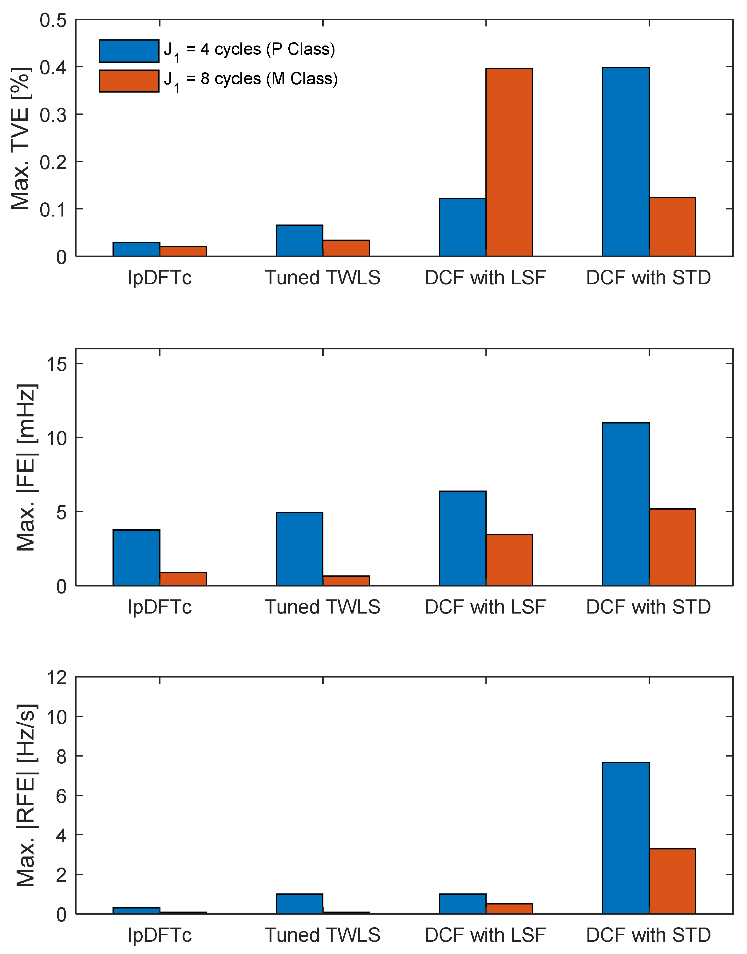
  • As far as synchrophasor estimation is concerned, all algorithms return maximum TVE values compliant with the Standard even over observation intervals so short as two nominal power line cycles. However, the IpDFTc and the tuned-TWLS algorithms provide the lowest TVE values. In particular, the IpDFTc algorithm is generally preferable in steady-state testing conditions and in the presence of wideband noise, whereas the tuned TWLS estimator is superior when dynamic disturbances (i.e., modulations and frequency ramps) are considered.
  • The estimation of the fundamental frequency is quite problematic. If just two cycles are observed, no estimator is able to meet the P Class |FE| limits reported in the Standard in all the testing conditions. In fact, further simulations showed that at least 3-cycle observation intervals are needed. In this scenario, the DCF approach with the STD filter seems to be globally preferable. If 4-cycle observation intervals are used, all estimators return results compliant with the Standard. The |FE| values are indeed comparable in most cases. However, the tuned TWLS approach appears slightly better than the others (and particularly much better than the IpDFTc under the effect of modulations).
  • Finally, as far as ROCOF estimation is concerned, the IpDFTc estimator is the only one that is able to meet the P Class |RFE| limits reported in the Standard by using both 2-cycle and 4-cycle observation intervals. The tuned TWLS approach over 2-cycle intervals returns accurate results in most cases, but it is strongly affected by the presence of harmonics. On the other hand, if 4-cycle observation intervals are used, the IpDFTc, the tuned TWLS, and the DCF approach with the LSF filter exhibit comparable performances.
Table 5a,b shows the maximum values of TVE, |FE| and |RFE| (computed over 1000 records) obtained over 6-cycle (a) or 8-cycle (b) observation intervals in the M Class testing conditions listed at the beginning of this Section. In this case, longer observation intervals are considered as they are needed to ensure a higher measurement accuracy. The M Class limits mentioned in the Standard (when defined) are also shown. The values exceeding such limits are highlighted in bold, whereas the cells containing the best results obtained in each test are shaded. Again, both the IpDFTc and the tuned TWLS algorithm rely on a Hann window. The LSF FIR filters used with the DCF approach is again based on least-squares frequency response error minimization assuming 6-cycle-long and 8-cycle-long impulse responses, respectively. On the contrary, the M Class STD filter suggested in Annex D of the Standard does no longer exhibit a triangular impulse response. In fact, it results from the classic window design method: the non-causal sinc-shaped impulse response of the ideal low-pass filter is indeed modulated by a Hamming window.
The results in Table 5a,b can be summarized as follows.
  • As far as synchrophasor estimation is concerned, the maximum TVE values basically confirm the conclusions drawn in the P Class case. The IpDFTc algorithm is generally preferable in steady-state testing conditions and in the presence of wideband noise, whereas the tuned TWLS estimator is superior when dynamic disturbances (i.e., modulations and frequency ramps) are considered. However, in the M Class case, such differences are exacerbated. The tuned TWLS approach is not able to meet the Standard limits in the presence of out-of-band inter-harmonics over 6-cycle intervals, but it meets the Standard requirements over 8-cycle intervals. Quite interestingly, the accuracy of the tuned TWLS algorithm over longer intervals under dynamic conditions slightly degrades due to the larger Taylor’s series approximation errors of the phasor model at the edges of the observation intervals [29]. The IpDFTc estimator is not able to meet the Standard limits over 8-cycle intervals when amplitude or phase oscillations perturb the fundamental component. Only the DCF approach is able to meet the Standard limits with both interval lengths, although in some testing conditions it exhibits a slightly worse accuracy than the other algorithms.
  • The |FE| values exhibit a trend similar to the TVE ones. The main difference is in the case of the DCF approach whose behavior is more heterogeneous. In this case, ensuring compliance with the Standard requirements is much more challenging. Indeed, no estimator is able to meet the Standard limits in the case of inter-harmonic interference over 6-cycle intervals. Over 8-cycle intervals instead, the IpDFTc estimator returns generally the best results except in the case of amplitude and phase modulations, which are more effectively mitigated by the DCF approach with the LSF filter.
  • Finally, in the case of ROCOF estimation, almost all algorithms except the DCF approach with the STD filter exhibit good results. They are indeed compliant with the limits reported in the Standard (when defined). Globally, the IpDFTc estimator is preferable over 6-cycle intervals, whereas the tuned TWLS algorithm is better over 8-cycle intervals in accordance with the TVE trend.

3.2. Results in Transient Conditions

To compare the behavior of the three considered IpDFT-tuned estimation algorithms in transient conditions, both the response times associated with synchrophasor, frequency and ROCOF estimation, and the measurement delay times are computed in the worst-case conditions specified in the Standard [10]. In this case, the testing conditions are: either amplitude step changes equal to ±10% of the nominal amplitude or phase step changes of ±10°. It is worth recalling that the response times are defined as the temporal intervals between the instants at which, as a result of a step input change, the measured values of synchrophasor, frequency or ROCOF exceed a specified TVE, |FE| or |RFE| threshold (i.e., 1%, 5 mHz or 0.4 Hz/s, respectively, in the case of P Class PMUs, or 1%, 5 mHz or 0.1 Hz/s in the case of M Class PMUs) and the times after which the measured values steadily remain under such thresholds.
During the transients, the maximum over- or undershoots affecting amplitude or phase estimates (depending on the type of applied input step) are also of interest, as they are required to be smaller than 5% or 10% of the input step size for P Class and M Class PMUs, respectively.
The measurement delay time is defined as “the time interval between the instant that a step change is applied to the input of a PMU and the measurement time when the stepped parameter achieves a value that is half-way between the initial and final steady-state values” [10].
In the present study, the P Class and M Class maximum response times and the maximum measurement delay times (obtained by shifting sample-by-sample the instants at which the steps occur) are shown in Table 6a,b over 2-cycle and 4-cycle observation intervals and in Table 7a,b over 6-cycle and 8-cycle observation intervals, respectively.
The results in both cases are quite consistent and can be summarized as follows:
  • The limits reported in the Standard are met in almost all cases with a few exceptions.
  • The maximum synchrophasor and ROCOF response times of the TWLS estimator are always considerably shorter than those of the IpDFTc estimator. However, the IpDFTc frequency estimation response times are generally the shortest ones, except under the effect of amplitude steps when 4-cycle observation intervals are considered. In fact, this is the sole testing condition in which the DCF approach outperforms the other estimators. Furthermore, the over- and undershoots obtained with the IpDFTc estimator are generally smoother than those of the other algorithms. In any case, the over- and undershoots of all considered algorithms are well below the limits reported in the Standard. Therefore, they are not reported for the sake of brevity.
  • As far as the measurement delay times are concerned, the tuned TWLS and the IpDFTc estimators exhibit similar performances, quite better than those of the DCF method. Moreover, they are well below the limits reported in the Standard [10].

4. Discussion

Table 8a,b summarizes the results of the performance analysis in the P Class and M Class testing conditions reported in Section 3. The estimation algorithms with TVE, |FE| and |RFE| values and with response times (in the case of amplitude or phase step changes) below the limits reported in the Standard in all the considered testing conditions are denoted as Compliant (C). If at least one of the TVE, |FE|, |RFE| or response time limits is exceeded, an estimator is labeled as Not Compliant (NC). Again, the algorithm with the best performances in estimating each parameter is highlighted by shading the corresponding cell in Table 8a,b. The criteria adopted to identify the best estimator of each parameter for a given observation interval length are the following:
  • an algorithm able to return fully compliant TVE, |FE|, |RFE| or response time values is considered to be better than another one exceeding even a single limit, regardless of the estimation errors associated with the individual tests;
  • if two algorithms exhibit a different number of C and NC tests, the one with a larger number of compliant results in different tests is considered the better one, regardless of the estimation errors in the individual tests;
  • if two algorithms exhibit the same amount of compliant or non-compliant tests, the algorithm with a higher number of more accurate results shown in Table 4, Table 5, Table 6 and Table 7 is regarded as the better one;
  • if two algorithms exhibit the same amount of compliant or non-compliant tests and they do not clearly outperform one another (e.g., because results are very similar or because the number of testing conditions in which they are better is the same), the estimators are considered to have an equivalent performance.
From the analysis of Table 8a it results clearly that in the P-Class testing conditions full compliance is achieved only with the Tuned TWLS estimator over 4-cycle intervals. However, this is also the most demanding algorithm from the computational point of view. The IpDFTc estimator requires a lower computational burden and it is globally the best one over 2-cycle intervals, although it suffers from excessive |FE| values in steady-state testing conditions. Over 4-cycle intervals instead, despite its high accuracy, the main problem of the IpDFTc algorithm is the excessive response time duration affecting synchrophasor estimation after step changes.
In the M-Class testing conditions summarized in Table 8b the IpDFTc estimator is globally the best one over 6-cycle observation intervals, but it again suffers from excessive |FE| values when out-of-band inter-harmonics are considered. On the contrary, the Tuned TWLS algorithm is confirmed to be both fully compliant and the best estimator over 8-cycle observation intervals. Quite interestingly, the DCF technique with the LSF filter over 8-cycle intervals ensures full compliance in all tests considered, despite its accuracy and responsiveness not being excellent in any test.

5. Experimental Results in a Practical Case Study

To validate the simulation-based performance comparison reported above in a case study of practical interest, 1000 2-cycle, 4-cycle, 6-cycle and 8-cycle data records of a waveform generated by a function generator Agilent 33220A were collected through a 12-bit data acquisition system (DAQ) NI6023E. Each generated waveform exhibits nominal normalized amplitude, initial phase chosen at random in the range [0, 2π], fundamental frequency within [47 Hz, 52 Hz] and a Total Harmonic Distortion (THD) of about 9.4%. The THD level purposely slightly exceeds the limit reported in the Standard EN 50160:2010 [33]. In particular, according to that Standard, the range [47 Hz, 52 Hz] shall never be exceeded, although in practice the system frequency is required to lie within [49.5 Hz, 50.5 Hz] for 95% of the time of a week. The THD instead must be not greater than 8% with the first 25 harmonics that have to be smaller than a value ranging from 0.5% to about 6% of the fundamental, depending on the harmonic order. In the current study, just the harmonics from the 2nd to the 7th ones are included. Their amplitude is equal to 2%, 5%, 1%, 6%, 0.5% and 5% of the fundamental, respectively. The values of amplitude, phase, frequency and ROCOF evaluated at the reference times were estimated a posteriori through a multi-harmonic sine-fitting procedure [40].
The bar diagram in Figure 2 shows the maximum TVE, |FE| and |RFE| values computed over all data records and associated with the IpDFTc algorithm, the tuned TWLS estimator and the DCF technique using either the LSF or the STD filter, respectively. Given that, as shown in Section 3 and Section 4, the best results as well as the full compliance of some algorithms are obtained over 4-cycle intervals in the P Class case and over 8-cycle intervals in the M Class case, respectively, the results obtained over 2-cycle and 6-cycle intervals are omitted here for the sake of brevity. Moreover, the TVE, |FE| and |RFE| values obtained over 2 cycle intervals are very large due to the large spectral leakage caused by the 2nd and 3rd harmonic.
The results in Figure 2 confirm that, despite the presence of a variety of uncertainty contributions (most notably the limited spectral purity of the adopted waveform generator, the limited effective resolution of the DAQ and the uncertainty associated with the reconstruction of the reference values of amplitude, phase, frequency and ROCOF) the behavior of the estimation algorithms under test is consistent with the simulation results shown in Table 4b and Table 5b. In particular, it is evident that:
  • the IpDFTc estimator exhibits the best accuracy both over 4-cycle and 8-cycle observation intervals, as expected since it is natively conceived to counteract the effect of the 2nd harmonic;
  • the tuned TWLS returns slightly worse results, but it is worth recalling that it behaves better in dynamic and transient testing conditions;
  • the DCF technique is outperformed with either filter although the results obtained using a 4-cycle-long LSF are not much worse than those achieved with the IpDFTc and the tuned TWLS estimators. Note that the TVE values of the DCF technique with the LSF over 8-cycle intervals are quite worse than those over 4 cycle-intervals. However, this behavior is consistent with the corresponding simulation results shown in Table 4b and Table 5b and this is probably due to the larger bandwidth of the LSF with an 8-cycle-long impulse response compared with the LSF with a 4-cycle-long impulse response. Indeed, while the latter filter is conceived for P Class applications, the former one is optimized not to perturb stronger amplitude and phase oscillations in the M Class case. Thus, the LSF with an 8-cycle-long impulse response makes the DCF technique more sensitive to noise (e.g., injected by the experimental tested).

6. Conclusions

Recent research results have shown that if a preliminary fundamental frequency measurement is performed to compensate for the effect of static off-nominal frequency deviations, the accuracy of some of the most common estimation algorithms for PMUs can be greatly improved. Till now, to the best of Authors’ knowledge, no clear performance comparisons between estimation algorithms exploiting the benefits of a preliminary frequency measurement have been reported in the scientific literature. In this paper, the performances of three alternative techniques for the estimation of AC waveform amplitude, phase, frequency and ROCOF based on an a prior 2-point Interpolated Discrete Fourier Transform (IpDFT) stage are evaluated in the very same P Class or M Class testing conditions specified in the IEEE/IEC Standard 60255-118-1:2018 and using data records of the same size. The algorithms considered in this study are: the corrected IpDFT (IpDFTc), the tuned Taylor Weighted Least Squares (TWLS) estimator, and the frequency Down-Conversion and low-pass Filtering (DCF) technique with two alternative types of low-pass filter. The performance comparison shows that the IpDFTc and the tuned TWLS methods are generally more accurate and exhibit shorter transients than the DCF technique, although the latter one still fulfills the Standard requirements in most testing conditions. Quite importantly, the behavior of the DCF algorithm is strongly affected by the chosen low-pass filter and it could be further improved by adopting custom optimization strategies for FIR filter design. The IpDFTc technique is preferable over short intervals and it overcomes the others when the analyzed waveform is affected by steady-state harmonic and inter-harmonic disturbances. However, it is considerably worse than the tuned TWLS estimator in the presence of amplitude or phase oscillations and it is not able to ensure compliance to the IEEE/IEC Standard in a few testing conditions. On the contrary, the tuned TWLS estimator is much more effective in dynamic conditions, it exhibits shorter synchrophasor and ROCOF response times (although with greater overshoots) and, assuming a reporting rate of 50 readings/s, it returns fully compliant results in the P Class and M Class tests described in the IEEE/IEC Standard over 4-cycle and 8-cycle observation intervals, respectively.

Author Contributions

Conceptualization, D.B., D.M. and D.P.; methodology, D.B., D.M. and D.P.; software, D.B. and D.M.; validation, D.B. and D.M.; writing—original draft preparation, D.B., D.M. and D.P. All authors have read and agreed to the published version of the manuscript.

Funding

This research received no external funding.

Institutional Review Board Statement

Not applicable.

Informed Consent Statement

Not applicable.

Conflicts of Interest

The authors declare no conflict of interest.

Appendix A. Analytical Expressions of the Elements of Vector P ^ r in (23)

In [28] it is shown that, if K = 2, the elements of vector P r ^ in (23) can be computed analytically in the frequency domain as follows, i.e.,
c ^ 1 , r ( 0 ) = α 33 R e { Y r , W 2 ( ν ^ 10 , r ) } α 35 2 π R e { Y r , W 2 ( 1 ) ( ν ^ 10 , r ) } α 13 4 π 2 R e { Y r , W 2 ( 2 ) ( ν ^ 10 , r ) } s ^ 1 , r ( 0 ) = α 44 I m { Y r , W 2 ( ν ^ 10 , r ) } + α 24 2 π I m { Y r , W 2 ( 1 ) ( ν ^ 10 , r ) } α 46 4 π 2 R e { Y r , W 2 ( 2 ) ( ν ^ 10 , r ) } , c ^ 1 , r ( 1 ) = α 24 I m { Y r , W 2 ( ν ^ 10 , r ) } α 22 2 π I m { Y r , W 2 ( 1 ) ( ν ^ 10 , r ) } + α 26 4 π 2 I m { Y r , W 2 ( 2 ) ( ν ^ 10 , r ) } , s ^ 1 , r ( 1 ) = α 35 R e { Y r , W 2 ( ν ^ 10 , r ) } + α 55 2 π R e { Y r , W 2 ( 1 ) ( ν ^ 10 , r ) } + α 15 4 π 2 R e { Y r , W 2 ( 2 ) ( ν ^ 10 , r ) } c ^ 1 , r ( 2 ) = α 13 R e { Y r , W 2 ( ν ^ 10 , r ) } α 15 2 π R e { Y r , W 2 ( 1 ) ( ν ^ 10 , r ) } α 11 4 π 2 R e { Y r , W 2 ( 2 ) ( ν ^ 10 , r ) } , s ^ 1 , r ( 2 ) = α 46 I m { Y r , W 2 ( ν ^ 10 , r ) } + α 26 2 π I m { Y r , W 2 ( 1 ) ( ν ^ 10 , r ) } α 66 4 π 2 I m { Y r , W 2 ( 2 ) ( ν ^ 10 , r ) } ,
where Y r , W 2 ( ν ) = def m = N h N h y r ( m ) w 2 ( m ) e j 2 π ν m is the DTFT of the r-th data record weighted by the squared window w2(·), Y r , W 2 ( k ) ( ν ) = def d k Y W 2 ( ν ) d ν k = ( j 2 π ) k m = N h N h m k y r ( m ) w 2 ( m ) e j 2 π ν m is its k-th order derivative, and coefficients αij, with i,j = 1, 2,…, 6, are given by: α 11 = c 1 2 a 0 b 2 Δ 1 , α 13 = c 1 c 3 a 2 b 2 Δ 1 , α 15 = a 2 c 1 c 3 a 0 Δ 1 , α 22 = b 2 2 b 0 b 4 Δ 2 , α 24 = c 1 b 4 c 3 b 2 Δ 2 , α 26 = c 1 b 2 b 0 c 3 Δ 2 , α 33 = c 3 2 a 4 b 2 Δ 1 , α 35 = a 4 c 1 a 2 c 3 Δ 1 , α 44 = c 3 2 a 2 b 4 Δ 2 , α 46 = c 1 c 3 a 2 b 2 Δ 2 , α 55 = a 2 2 a 0 a 4 Δ 1 , α 66 = c 1 2 b 0 a 2 Δ 2 , in which Δ 1 = a 4 c 1 2 2 a 2 c 3 c 1 + b 2 a 2 2 + a 0 c 3 2 a 0 b 2 a 4 ,   Δ 2 = b 4 c 1 2 2 b 2 c 3 c 1 + a 2 b 2 2 + b 0 c 3 2 a 2 b 0 b 4 , where
a 0 = m = N h N h w 2 ( m ) cos 2 ( 2 π ν ^ 10 , r m ) , a 2 = m = N h N h m 2 w 2 ( m ) cos 2 ( 2 π ν ^ 10 , r m ) , a 4 = m = N h N h m 4 w 2 ( m ) cos 2 ( 2 π ν ^ 10 , r m ) ,     b 0 = m = N h N h w 2 ( m ) sin 2 ( 2 π ν ^ 10 , r m ) , b 2 = m = N h N h m 2 w 2 ( m ) sin 2 ( 2 π ν ^ 10 , r m ) , b 4 = m = N h N h m 4 w 2 ( m ) sin 2 ( 2 π ν ^ 10 , r m ) , c 1 = 0.5 m = N h N h m w 2 ( m ) sin ( 4 π ν ^ 10 , r m ) , c 3 = 0.5 m = N h N h m 3 w 2 ( m ) sin ( 4 π ν ^ 10 , r m ) .

References

  1. Phadke, A.G.; Thorp, J.S.; Adamiak, M.G. A New Measurement Technique for Tracking Voltage Phasors, Local System Frequency, and Rate of Change of Frequency. IEEE Trans. Power Appar. Syst. 1983, PAS-102, 1025–1038. [Google Scholar] [CrossRef]
  2. Laverty, D.M.; Best, R.J.; Morrow, D.J. Loss-of-mains protection system by application of phasor measurement unit technology with experimentally assessed threshold settings. IET Gener. Transm. Distrib. 2015, 9, 146–153. [Google Scholar] [CrossRef] [Green Version]
  3. Borghetti, A.; Nucci, C.A.; Paolone, M.; Ciappi, G.; Solari, A. Synchronized Phasors Monitoring During the Islanding Maneuver of an Active Distribution Network. IEEE Trans. Smart Grid 2011, 2, 82–91. [Google Scholar] [CrossRef] [Green Version]
  4. Pignati, M.; Zanni, L.; Romano, P.; Cherkaoui, R.; Paolone, M. Fault Detection and Faulted Line Identification in Active Distribution Networks Using Synchrophasors-Based Real-Time State Estimation. IEEE Trans. Power Deliv. 2017, 32, 381–392. [Google Scholar] [CrossRef] [Green Version]
  5. Aslanian, M.; Hamedani-Golshan, M.E.; Haes Alhelou, H.; Siano, P. Analyzing Six Indices for Online Short-Term Voltage Stability Monitoring in Power Systems. Appl. Sci. 2020, 10, 4200. [Google Scholar] [CrossRef]
  6. Liu, J.; Tang, J.; Ponci, F.; Monti, A.; Muscas, C.; Pegoraro, P.A. Trade-Offs in PMU Deployment for State Estimation in Active Distribution Grids. IEEE Trans. Smart Grid 2012, 3, 915–924. [Google Scholar] [CrossRef]
  7. Kong, X.; Chen, Y.; Xu, T.; Wang, C.; Yong, C.; Li, P.; Yu, L. A Hybrid State Estimator Based on SCADA and PMU Measurements for Medium Voltage Distribution System. Appl. Sci. 2018, 8, 1527. [Google Scholar] [CrossRef] [Green Version]
  8. Zanni, L.; Derviškadić, A.; Pignati, M.; Xu, C.; Romano, P.; Cherkaoui, R.; Abur, A.; Paolone, M. PMU-based linear state estimation of Lausanne subtransmission network: Experimental validation. Electr. Power Syst. Res. 2020, 189, 1–7. [Google Scholar] [CrossRef]
  9. Lin, C.; Wu, W.; Guo, Y. Decentralized Robust State Estimation of Active Distribution Grids Incorporating Microgrids Based on PMU Measurements. IEEE Trans. Smart Grid 2020, 11, 810–820. [Google Scholar] [CrossRef]
  10. IEC/IEEE 60255-118-1:2018, IEEE/IEC International Standard—Measuring Relays and Protection Equipment—Part 118-1: Synchrophasor for Power Systems—Measurements. 2018, pp. 1–78. Available online: https://webstore.iec.ch/preview/info_iecieee60255-118-1%7Bed1.0%7Den.pdf (accessed on 4 March 2021).
  11. Biswal, M.; Brahma, S.M.; Cao, H. Supervisory Protection and Automated Event Diagnosis Using PMU Data. IEEE Trans. Power Deliv. 2016, 31, 1855–1863. [Google Scholar] [CrossRef]
  12. Kim, J.; Kim, H.; Choi, S. Performance Criterion of Phasor Measurement Units for Distribution System State Estimation. IEEE Access 2019, 7, 106372–106384. [Google Scholar] [CrossRef]
  13. Barchi, G.; Fontanelli, D.; Macii, D.; Petri, D. On the Accuracy of Phasor Angle Measurements in Power Networks. IEEE Trans. Instrum. Meas. 2015, 64, 1129–1139. [Google Scholar] [CrossRef]
  14. Luiso, M.; Macii, D.; Tosato, P.; Brunelli, D.; Gallo, D.; Landi, C. A Low-Voltage Measurement Testbed for Metrological Characterization of Algorithms for Phasor Measurement Units. IEEE Trans. Instrum. Meas. 2018, 67, 2420–2433. [Google Scholar] [CrossRef]
  15. Tang, Y.; Stenbakken, G.N.; Goldstein, A. Calibration of Phasor Measurement Unit at NIST. IEEE Trans. Instrum. Meas. 2013, 62, 1417–1422. [Google Scholar] [CrossRef]
  16. Frigo, G.; Colangelo, D.; Derviskadic, A.; Pignati, M.; Narduzzi, C.; Paolone, M. Definition of Accurate Reference Synchrophasors for Static and Dynamic Characterization of PMUs. IEEE Trans. Instrum. Meas. 2017, 66, 2233–2246. [Google Scholar] [CrossRef]
  17. Belega, D.; Petri, D. Accuracy Analysis of the Multicycle Synchrophasor Estimator Provided by the Interpolated DFT Algorithm. IEEE Trans. Instrum. Meas. 2013, 62, 942–953. [Google Scholar] [CrossRef]
  18. Macii, D.; Petri, D.; Zorat, A. Accuracy Analysis and Enhancement of DFT-Based Synchrophasor Estimators in Off-Nominal Conditions. IEEE Trans. Instrum. Meas. 2012, 61, 2653–2664. [Google Scholar] [CrossRef]
  19. Agrez, D. Weighted multipoint interpolated DFT to improve amplitude estimation of multifrequency signal. IEEE Trans. Instrum. Meas. 2002, 51, 287–292. [Google Scholar] [CrossRef]
  20. Borkowski, J.; Kania, D.; Mroczka, J. Interpolated-DFT-Based Fast and Accurate Frequency Estimation for the Control of Power. IEEE Trans. Ind. Electron. 2014, 61, 7026–7034. [Google Scholar] [CrossRef]
  21. Radil, T.; Ramos, P.M.; Cruz Serra, A. New Spectrum Leakage Correction Algorithm for Frequency Estimation of Power System Signals. IEEE Trans. Instrum. Meas. 2009, 58, 1670–1679. [Google Scholar] [CrossRef]
  22. Belega, D.; Macii, D.; Petri, D. Power System Frequency Estimation Accuracy of Improved DFT-based Algorithms over Short Intervals. In Proceedings of the 2016 IEEE International Workshop on Applied Measurements for Power Systems (AMPS), Aachen, Germany, 27–29 September 2016; pp. 1–6. [Google Scholar]
  23. Wen, H.; Li, C.; Yao, W. Power System Frequency Estimation of Sine-Wave Corrupted With Noise by Windowed Three-Point Interpolated DFT. IEEE Trans. Smart Grid 2018, 9, 5163–5172. [Google Scholar] [CrossRef]
  24. Singh, A.K.; Pal, B.C. Rate of Change of Frequency Estimation for Power Systems Using Interpolated DFT and Kalman Filter. IEEE Trans. Power Syst. 2019, 34, 2509–2517. [Google Scholar] [CrossRef]
  25. Romano, P.; Paolone, M. Enhanced Interpolated-DFT for Synchrophasor Estimation in FPGAs: Theory, Implementation, and Validation of a PMU Prototype. IEEE Trans. Instrum. Meas. 2014, 63, 2824–2836. [Google Scholar] [CrossRef]
  26. Derviskadic, A.; Romano, P.; Paolone, M. Iterative-Interpolated DFT for Synchrophasor Estimation: A Single Algorithm for P- and M-Class Compliant PMUs. IEEE Trans. Instrum. Meas. 2018, 67, 547–558. [Google Scholar] [CrossRef] [Green Version]
  27. Belega, D.; Petri, D. Fast Procedures for Accurate Parameter Estimation of Sine-waves Affected by Noise and Harmonic Distortion. Digit. Signal Process 2021. under review. [Google Scholar]
  28. Belega, D.; Fontanelli, D.; Petri, D. Low-Complexity Least-Squares Dynamic Synchrophasor Estimation Based on the Discrete Fourier Transform. IEEE Trans. Instrum. Meas. 2015, 64, 3284–3296. [Google Scholar] [CrossRef]
  29. Tosato, P.; Macii, D.; Luiso, M.; Brunelli, D.; Gallo, D.; Landi, C. A Tuned Lightweight Estimation Algorithm for Low-Cost Phasor Measurement Units. IEEE Trans. Instrum. Meas. 2018, 67, 1047–1057. [Google Scholar] [CrossRef]
  30. Platas-Garza, M.A.; de la O Serna, J.A. Dynamic Phasor and Frequency Estimates through Maximally Flat Differentiators. IEEE Trans. Instrum. Meas. 2010, 59, 1803–1811. [Google Scholar] [CrossRef]
  31. Platas-Garza, M.A.; de la O Serna, J.A. Dynamic Harmonic Analysis through Taylor–Fourier Transform. IEEE Trans. Instrum. Meas. 2011, 60, 804–813. [Google Scholar] [CrossRef]
  32. Macii, D.; Petri, D. Digital Filters for Phasor Measurement Units: Design Criteria, Advantages and Limitations. In Proceedings of the 2019 IEEE 10th International Workshop on Applied Measurements for Power Systems (AMPS), Aachen, Germany, 25–27 September 2019; pp. 1–6. [Google Scholar]
  33. EN 50160:2010, Voltage Characteristics of Electricity Supplied by Public Distribution Systems, Brussels, Belgium, 2010.
  34. Harris, F.J. On the Use of Windows for Harmonic Analysis with the Discrete Fourier Transform. Proc. IEEE 1978, 66, 51–83. [Google Scholar] [CrossRef]
  35. Nuttall, A.H. Some windows with very good sidelobe behavior. IEEE Trans. Acoust. Speech Signal Process. 1981, ASSP-29, 84–91. [Google Scholar] [CrossRef] [Green Version]
  36. Belega, D.; Dallet, D. Multifrequency signal analysis by Interpolated DFT method with maximum sidelobe decay windows. Measurement 2009, 42, 420–426. [Google Scholar] [CrossRef]
  37. Macii, D.; Barchi, G.; Petri, D. Design criteria of digital filters for synchrophasor estimation. In Proceedings of the IEEE International Instrumentation and Measurement Technology Conference (I2MTC), Minneapolis, MN, USA, 6–9 May 2013; pp. 1579–1584. [Google Scholar]
  38. Messina, F.; Vega, L.R.; Marchi, P.; Galarza, C.G. Optimal Differentiator Filter Banks for PMUs and Their Feasibility Limits. IEEE Trans. Instrum. Meas. 2017, 66, 2948–2956. [Google Scholar] [CrossRef]
  39. Macii, D.; Fontanelli, D.; Barchi, G.; Petri, D. Impact of Acquisition Wideband Noise on Synchrophasor Measurements: A Design Perspective. IEEE Trans. Instrum. Meas. 2016, 65, 2244–2253. [Google Scholar] [CrossRef]
  40. Ramos, P.M.; da Silva, M.F.; Martins, R.C.; Cruz Serra, A.M. Simulation and Experimental Results of Multiharmonic Least-Squares Fitting Algorithms Applied to Periodic Signals. IEEE Trans. Instrum. Meas. 2006, 55, 646–651. [Google Scholar] [CrossRef]
Figure 1. Maximum TVE, |FE|, and |RFE| values over 1000 records of 6-cycle and 8-cycle observation intervals obtained with the classic IpDFT and the IpDFTc estimators as a function of the off-nominal frequency deviations assuming that the first 50 harmonics of amplitude equal to 10% of the fundamental component affect the collected waveform.
Applsci 11 02318 g001
Figure 2. Maximum TVE, |FE|, and |RFE| values obtained with the IpDFTc algorithm, the tuned TWLS estimator and the DCF technique (using either the LSF or the STD filter), over 1000 experimental 4-cycle and 8-cycle data records with system frequency in the range [47 Hz, 52 Hz] and THD ≈ 9.4%. The THD level slightly exceeds the limits specified in the Standard EN.
Applsci 11 02318 g002
Table 1. Steps of the IpDFTc estimation algorithm for PMUs.
Step 1:
Apply the IpDFT algorithm based on the Hann window to the r-th data record yr(·) and determine the estimators ν ^ 10 , r ,   a ^ 10 , r ,   and   ϕ ^ 10 , r by using (7) and (9).
Step 2:
Compute the residual signal y ˜ r ( · ) by removing the estimated sinewave from the acquired samples yr(·).
Step 3:
Apply the IpDFT algorithm based on the Hann window again to the residual signal y ˜ r ( · ) and determine the second harmonic parameters ν ^ 20 , r ,   a ^ 20 , r ,   and   ϕ ^ 20 , r .
Step 4:
Compute the new sine-wave parameter estimates ν ^ 1 , r ,   a ^ 1 , r ,   and   ϕ ^ 1 , r by using (11), (15), and (16).
Step 5:
Compute f 1 , r and R O C O F ^ 1 , r by using (17) and (18).
Step 6:
Return the estimated parameters.
Table 2. Steps of the tuned real-valued TWLS estimation algorithm for PMUs.
Step 1:
Apply the IpDFT algorithm based on the Hann window to the r-th data record yr(·) and determine the estimator ν ^ 10 , r from (7).
Step 2:
Compute the elements of the vector P r ^ through (23).
Step 3:
Compute the estimators a ^ 1 , r   and   ϕ ^ 1 , r by (24), and the estimators of f ^ 1 , r and R O C O F ^ 1 , r with (25) and (26), respectively.
Step 4:
Return the estimated parameters.
Table 3. Steps of the tuned DCF estimation algorithm for PMUs.
Step 1:
Apply the IpDFT algorithm based on the Hann window to the r-th data record yr(·) and determine the estimator ν ^ 10 , r from (7).
Step 2:
Mix the samples of the data record yr(·) with two quadrature sinewaves of unit amplitude and frequency f ^ 1 , r = ν ^ 10 , r · f s /M to obtain the I/Q components of the collected signal.
Step 3:
Apply a suitable low-pass filter to the I/Q components to remove disturbances and the double-frequency terms.
Step 4:
Compute the estimators a ^ 1 , r   and   ϕ ^ 1 , r by (29), and the estimators f ^ 1 , r and R O C O F ^ 1 , r with (30) and (31), respectively.
Step 5:
Return the estimated parameters.
Table 4. Maximum TVE, |FE|, and |RFE| values obtained with the estimation algorithms for PMUs described in Section 2 over 2-cycle (a) or 4-cycle (b) observation intervals. All the testing conditions, except the one with the additive wideband noise, are specified in the IEEE/IEC Standard 60255-118-1:2018 for P Class PMUs [10]. The limits mentioned in the Standard (when defined) are also reported. The values exceeding such limits are highlighted in bold, whereas the cells containing the best results obtained in each test are shaded.
(a)
Test TypeTVEmax(%)|FE|max(mHz)|RFE|max(Hz/s)
Lim.IpDFTcTuned TWLSDCFLim.IpDFTcTuned
TWLS
DCFLim.IpDFTcTuned
TWLS
DCF
LSFSTDLSFSTDLSFSTD
Freq. dev. only (±2 Hz)10.010.000.380.1758.917.713.57.20.40.20.08.14.2
Freq. dev.+ 1% harmonics10.010.740.380.17510.614114.17.50.40.354.78.44.8
AM (fa = 2 Hz, ka = 10%)30.040.000.360.05608.00.00.00.02.30.10.00.00.0
PM (fp = 2 Hz, kp = 0.1 rad)30.040.000.370.03601.80.51.60.72.30.00.00.60.0
Freq. ramp 1 (±2 Hz @ ±1 Hz/s)10.020.000.400.19105.410.813.97.20.40.10.08.04.2
AWGN (SNR = 60 dB)-0.030.040.360.03-14.124.32.72.5-0.61.40.30.3
(b)
Test TypeTVEmax(%)|FE|max(mHz)|RFE|max(Hz/s)
Lim.IpDFTcTunedTWLSDCFLim.IpDFTcTuned
TWLS
DCFLim.IpDFTcTuned
TWLS
DCF
LSFSTDLSFSTDLSFSTD
Freq. dev. only (±2 Hz)10.000.030.060.1650.10.10.46.30.40.00.00.33.8
Freq. dev.+ 1% harmonics10.000.010.060.1650.11.40.46.50.40.00.30.34.0
AM (fa = 2 Hz, ka = 10%)30.150.000.090.156014.30.00.00.12.30.20.00.00.3
PM (fp = 2 Hz, kp = 0.1 rad)30.160.000.060.12602.11.80.42.02.30.00.00.00.0
Freq. ramp 1 (±2 Hz @ ±1 Hz/s)10.070.030.060.21100.10.10.56.30.40.00.00.43.8
AWGN (SNR = 60 dB)-0.020.030.090.02-2.93.52.92.2-0.20.30.30.1
1 Results obtained considering an exclusion interval of 40 ms (i.e., twice the maximum mandatory reporting period at 50 Hz) at the beginning and at the end of the frequency ramp.
Table 5. Maximum TVE, |FE| and |RFE| values obtained with the estimation algorithms for PMUs described in Section 2 over 6-cycle (a) and 8-cycle (b) observation intervals. All the testing conditions, except the one with the additive wideband noise, are specified in the IEEE/IEC Standard 60255-118-1:2018 for M Class PMUs [10]. The limits mentioned in the Standard (when defined) are also reported. The values exceeding such limits are highlighted in bold, whereas the cells containing the best results obtained in each test are shaded.
(a)
Test TypeTVEmax(%)|FE|max(mHz)|RFE|max(Hz/s)
Lim.IpDFTcTunedTWLSDCFLim.IpDFTcTuned
TWLS
DCFLim.IpDFTcTuned
TWLS
DCF
LSFSTDLSFSTDLSFSTD
Freq. dev. only (±5 Hz)10.000.000.330.1350.00.017.08.40.40.00.09.84.7
Freq. dev.+ 10% harmonics10.000.020.340.1350.10.221.110.20.40.00.312.16.5
AM (fa = 5 Hz, ka = 10%)32.360.070.490.893001405.21.52.3144.20.13.48.1
PM (fp = 5 Hz, kp = 0.1 rad)32.120.070.320.6930070.459.09.636.4142.11.71.51.9
Freq. ramp 1 (±5 Hz @ ±1 Hz/s)10.150.000.290.20100.00.11.29.00.40.00.00.14.0
AWGN (SNR = 60 dB)-0.020.030.330.02-1.31.614.11.0-0.10.19.10.1
10% inter-harmonics1.30.082.320.570.541025.510057.670.9-2.523.612.612.3
(b)
Test TypeTVEmax(%)|FE|max(mHz)|RFE|max(Hz/s)
Lim.IpDFTcTunedTWLSDCFLim.IpDFTcTuned
TWLS
DCFLim.IpDFTcTuned
TWLS
DCF
LSFSTDLSFSTDLSFSTD
Freq. dev. only (±5 Hz)10.000.000.340.1150.00.000.79.90.40.00.00.45.7
Freq. dev.+ 10% harmonics10.000.000.340.1250.00.20.711.40.40.00.00.46.5
AM (fa = 5 Hz, ka = 10%)33.920.210.431.46300164.79.90.54.2144.90.12.217.8
PM (fp = 5 Hz, kp = 0.1 rad)33.510.200.351.21300119.2100.34.159.9143.62.80.22.4
Freq. ramp 1 (±5 Hz @ ±1 Hz/s)10.260.000.370.20100.10.11.29.90.40.00.00.45.8
AWGN (SNR = 60 dB)-0.020.020.350.20-0.91.20.80.7-0.10.10.50.0
10% inter-harmonics1.30.020.020.380.12103.66.57.77.8-0.40.31.33.0
1 Results obtained considering an exclusion interval of 140 ms (i.e., 7 times the maximum mandatory reporting period at 50 Hz) at the beginning and at the end of the ramp.
Table 6. Maximum response times (expressed in nominal power line cycles) associated with synchrophasor, frequency and ROCOF estimation (a) and maximum delay times (b), under the influence of the worst-case amplitude or phase step changes specified in the IEEE/IEC Standard 60255-118-1:2018 for P Class PMUs using 2-cycle or 4-cycle observation intervals. The limits specified in the Standard are also shown. The values exceeding the limits are highlighted in bold, whereas the cells containing the best results obtained in each test are shaded.
(a)
Test TypeObs. Inter. Length
[cycles]
Synchrophasor Resp. Time
(cycles)
Frequency Resp. Time (cycles)ROCOF Resp. Time (cycles)
LimIpDFTcTuned TWLSDCFLim.IpDFTcTuned TWLSDCFLim.IpDFTcTuned
TWLS
DCF
LSFSTDLSFSTDLSFSTD
±10% amp. step221.050.561.231.184.51.841.889.152.7662.891.809.322.98
421.990.941.042.294.53.563.662.734.4564.683.437.974.91
±10° phase step221.251.001.351.434.51.851.889.252.8862.881.849.352.99
422.351.101.202.684.53.473.614.334.7464.643.588.184.98
(b)
Test TypeObs. Inter.
[cycles]
|Delay Time| (ms)
Lim.IpDFTcTuned TWLSDCF
LSFSTD
±10% amp. step251.501.673.001.80
451.501.501.801.80
±10° phase step251.832.004.702.80
451.831.832.002.50
Table 7. Maximum response times (expressed in nominal power line cycles) associated with synchrophasor, frequency and ROCOF estimation (a) and maximum delay times (b), under the influence of the worst-case amplitude or phase step changes specified in the IEEE/IEC Standard 60255-118-1:2018 for M Class PMUs using 6-cycle or 8-cycle observation intervals. The limits specified in the Standard are also shown. The values exceeding the limits are highlighted in bold, whereas the cells containing the best results obtained in each test are shaded.
(a)
Test TypeObs. Inter.
(cycles)
Synchrophasor Resp. Time
(cycles)
Frequency Resp. Time (cycles)ROCOF Resp. Time (cycles)
LimIpDFTcTuned TWLSDCFLim.IpDFTcTuned TWLSDCFLim.IpDFTcTuned
TWLS
DCF
LSFSTDLSFSTDLSFSTD
±10% amp. step672.961.361.681.98145.175.375.784.14146.434.907.3312.27
873.931.781.812.60146.716.994.374.96148.096.178.988.91
±10° phase step673.491.561.942.32145.135.317.136.36146.365.227.3312.28
874.632.042.173.06146.666.967.117.23148.056.788.988.91
(b)
Test TypeObs. Inter.
[cycles]
|Delay Time| (ms)
Lim.IpDFTcTuned TWLSDCF
LSFSTD
±10% amp. step651.501.501.501.50
851.501.502.202.00
±10° phase step651.831.834.804.50
851.831.833.004.70
Table 8. Overall comparison between the IpDFT-tuned estimation algorithms under study in the P Class (a) and M Class (b) PMU testing conditions reported in the IEEE/IEC Standard 60255-118-1:2018. Letter C stands for “full compliance” with all the limits reported in the testing conditions considered in Section 3 for RR = 50 frame/s, whereas “not compliant” (NC) means that at least one of the Standard limits is exceeded. The cells related to the best performing algorithm are shaded.
(a)
Estimation AlgorithmNo. CyclesTVE|FE||RFE|Phasor Resp. TimeFreq. Resp. TimeROCOF Resp. TimeDelay
Time
IpDFTc2CNCCCCCC
4CCCNCCCC
Tuned TWLS2CNCNCCCCC
4CCCCCCC
DCF with LSF2CNCNCCNCNCC
4CCCCCNCC
DCF with STD2CNCNCCCCC
4CNCNCNCNCCC
(b)
Estimation AlgorithmNo. CyclesTVE|FE||RFE|Phasor Resp. TimeFreq. Resp. TimeROCOF Resp. TimeDelay
Time
IpDFTc6CNCCCCCC
8NCCCCCCC
Tuned TWLS6NCNCCCCCC
8CCCCCCC
DCF with LSF6CNCNCCCCC
8CCCCCCC
DCF with STD6CNCNCCCCC
8CNCNCCCCC
Publisher’s Note: MDPI stays neutral with regard to jurisdictional claims in published maps and institutional affiliations.

