Numerical Investigation of Tonal Trailing-Edge Noise Radiated by Low Reynolds Number Airfoils

Abstract

A high-fidelity computational analysis carefully validated against concurrently obtained experimental results is employed to examine self-noise radiation of airfoils at transitional flow regimes, with a focus on elucidating the connection between the unsteady behavior of the laminar separation bubble (LSB) and the acoustic feedback-loop (AFL) resonant interactions observed in the airfoil boundary layers. The employed parametric study examines AFL sensitivity to the changes in the upstream flow conditions and the airfoil loading. Implicit Large-Eddy Simulations are performed for a NACA-0012 airfoil in selected transitional-flow regimes for which experimental measurements recorded characteristic multiple-tone acoustic spectra with a dual ladder-type frequency structure. The switch between the tone-producing and no-tone-producing regimes is traced to the LSB size and position as a function of the flow Reynolds number and the airfoil angle of attack, and further substantiated by the linear stability analysis. The results indicate a strong multi-tonal airfoil noise radiation associated with the AFL and attributed to the switch from the slowly-growing Tollmien–Schlichting to the fast-growing Kelvin–Helmholtz instabilities occurring in thin LSB regions when those are localized near the trailing-edge (TE) on either side of the airfoil. Such a process eventually results in the nonlinearly saturated flapping vortical modes (“rollers”) that scatter into acoustic waves at the TE.

1. Introduction

The noise generated by airfoils under specific low Reynolds number flow regimes have been historically documented by Paterson et al. [1], Tam [2], and Arbey and Bataille [3] to be well over 30 dB higher relative to the optimally designed operating condition. At such levels, the radiated sound (typically a combination of airfoil self-noise and tonal noise) can become extremely discomforting for individuals living nearby wind turbines or those operating small gliders. Ongoing efforts to mitigate the noise associated with long and slender wings used in wind turbines and gliders have initiated programs by large corporations, such as GE, to support research and development of more consumer-friendly products. In addition to the civil applications, the military sectors have also voiced concerns regarding the detectability of aircrafts, being a critical issue for Micro Air Vehicles (MAV) and Unmanned Air Vehicles (UAV) deployed on intelligence, surveillance, and reconnaissance (ISR) missions.

Throughout the years, significant research efforts (as reviewed, e.g., in Nash et al. [4], Desquesnes et al. [5], Kingan and Pearse [6], Plogmann et al. [7], Golubev et al. [8], Tam and Ju [9], and Yakhina et al. [10]) contributed towards elucidating the mechanisms responsible for airfoil trailing-edge (TE) noise generation. Although much has been accomplished in understanding the airfoil self-noise sources, the exact genesis of the tonal noise production and its connection to the acoustic feedback-loop process still requires further clarification. Thus, the current work focuses on numerically investigating the underlying physical phenomena and their effects on the mechanisms responsible for the generation of airfoil tonal noise in transitional flow regimes. To achieve this, the paper is organized as follows. In Section 2, we first reference the concurrent experimental study employed for validation of our numerical analysis. As the current work focuses on an Implicit Large-Eddy Simulations (ILES) approach for numerical experiments, the method and its implementation are discussed in detail. The validation of the 2D numerical analysis through comparison with 3D results is presented in Section 3. Section 4 is split into multiple parts describing the effects of the angle of attack (AoA) and Reynolds number (Re_c) on the airfoil transition from the tone-producing to no-tone-producing regimes, with the focus on the linear-stability analysis of the behavior of the laminar separation bubble (LSB) and evolution of viscous/inviscid instabilities during the transition process. The frequency selection process and the resulting spectral ladder-type frequency staging are examined as well. The final discussion of the obtained results is presented in Section 5.

2. Experimental and Numerical Approaches

2.1. Experimental Approach

The concurrent experimental measurements employed for validation in this work were carried out in an anechoic low-speed wind tunnel facility at Ecole Centrale de Lyon (ECL), with the details of the two conducted experimental campaigns described in Golubev et al. [8] and Yakhina et al. [10]. The tonal signature of the low-speed NACA-0012 airfoil was examined for a range of transitional flow regimes characterized by variable flow velocity, AoA, and unsteady inflow conditions to allow for thorough mapping of the regions of tonal production, including the effects of upstream unsteadiness. Figure 1 illustrates the locations of the Remote Microphone Probes (RMPs) in the experimental measurements (Golubev et al. [8]), where the surface pressure data were collected and employed for validation in the current numerical study. For velocity measurements, a hot-wire anemometer methodology was utilized.

2.2. Numerical Approach

2.2.1. High-Fidelity ILES Model

The employed ILES code (Visbal and Gaitonde [11]) solves a set of the compressible Navier–Stokes equations represented in a strong, conservative, time-dependent form in the generalized curvilinear computational coordinates (ξ, η, ζ, τ) transformed from the physical coordinates (x, y, z, t), where i and v denote inviscid and viscous terms, respectively.

$$\frac{\partial }{\partial \tau }(\frac{\overrightarrow{Q}}{J})+\frac{\partial {\overrightarrow{F}}_i}{\partial \xi }+\frac{\partial {\overrightarrow{G}}_i}{\partial \eta }+\frac{\partial {\overrightarrow{H}}_i}{\partial \zeta }+\frac{1}{\mathrm{Re}}[\frac{\partial {\overrightarrow{F}}_v}{\partial \xi }+\frac{\partial {\overrightarrow{G}}_v}{\partial \eta }+\frac{\partial {\overrightarrow{H}}_v}{\partial \zeta }]=\overrightarrow{S}$$

(1)

The solution vector $\overrightarrow{Q}=(\rho ,\rho u,\rho v,\rho w,\rho e)$ is defined in terms of the flow density $\rho$, Cartesian flow velocity components (u, v, w), and flow specific energy,

$$e=\frac{T}{\gamma (\gamma -1)M_{\infty }^2}+\frac{1}{2}(u^2+v^2+w^2)$$

(2)

with the assumed perfect gas relationship $p=\rho T/\gamma M_{\infty }^2$ connecting the flow pressure p, temperature T, and the freestream Mach number M_∞ (γ is the specific heat ratio). The other variables in Equation (1) include the inviscid flux vectors defined by

$${\overrightarrow{F}}_i=\left[\begin{array}{l}\rho \widehat{u}\\ \rho u\widehat{u}+{\widehat{\xi }}_{x}p\\ \rho v\widehat{u}+{\widehat{\xi }}_{y}p\\ \rho w\widehat{u}+{\widehat{\xi }}_{z}p\\ (\rho e+p)\widehat{u}-{\widehat{\xi }}_{t}p\end{array}\right],{\overrightarrow{G}}_i=\left[\begin{array}{l}\rho \widehat{v}\\ \rho u\widehat{v}+{\widehat{\eta }}_{x}p\\ \rho v\widehat{v}+{\widehat{\eta }}_{y}p\\ \rho w\widehat{v}+{\widehat{\eta }}_{z}p\\ (\rho e+p)\widehat{v}-{\widehat{\eta }}_{t}p\end{array}\right],{\overrightarrow{H}}_i=\left[\begin{array}{l}\rho \widehat{w}\\ \rho u\widehat{w}+{\widehat{\zeta }}_{x}p\\ \rho v\widehat{w}+{\widehat{\zeta }}_{y}p\\ \rho w\widehat{w}+{\widehat{\zeta }}_{z}p\\ (\rho e+p)\widehat{w}-{\widehat{\zeta }}_{t}p\end{array}\right]$$

(3)

where the transformation Jacobian is $J=\partial (\xi ,\eta ,\zeta ,\tau )/\partial (x,y,z,t)$, the metric quantities defined, e.g., as ${\widehat{\xi }}_x=(J^{-1})\partial \xi /\partial x$, etc., and the transformed flow velocity components are

$$\begin{array}{l}\widehat{u}={\widehat{\xi }}_t+{\widehat{\xi }}_{x}u+{\widehat{\xi }}_{y}v+{\widehat{\xi }}_{z}w\\ \widehat{v}={\widehat{\eta }}_t+{\widehat{\eta }}_{x}u+{\widehat{\eta }}_{y}v+{\widehat{\eta }}_{z}w\\ \widehat{w}={\widehat{\zeta }}_t+{\widehat{\zeta }}_{x}u+{\widehat{\zeta }}_{y}v+{\widehat{\zeta }}_{z}w\end{array}$$

(4)

The viscous flux vectors, ${\overrightarrow{F}}_v$, ${\overrightarrow{G}}_v$ and ${\overrightarrow{H}}_v$, are defined, e.g., in Anderson et al. [12], while $\overrightarrow{S}$ represents the source term that allows incompressible unsteady vortical perturbation to be introduced into the flow field. All flow variables are normalized by their respective reference freestream values except for pressure, which is nondimensionalized by ${\rho }_{\infty }{u}_{\infty }^2$.

Note that the governing equations are represented in the original unfiltered form, used unchanged in the laminar, transitional or fully turbulent regions of the flow, with Visbal et al. [13] providing further details on the code’s employed ILES procedure in which a high-order, low-pass filter operator is applied to the dependent variables during the solution process, in contrast to the standard LES addition of sub-grid stress (SGS) and heat flux terms. The resulting filter selectively damps the evolving poorly resolved high-frequency content of the solution.

The code employs a finite-difference approach to discretize the governing equations, with all the spatial derivatives obtained using the high-order compact-differencing schemes from Lele [14]. For the airfoil computations of the current paper, a 6th-order scheme is used. At boundary points, higher-order, one-sided formulas are utilized to retain the tridiagonal form of the scheme. In order to ensure that the Geometric Conservation Law (GCL) is satisfied, the time metric terms are evaluated employing the procedures described in detail in Visbal and Gaitonde [11]. Finally, the time marching is accomplished by incorporating a 2nd-order, iterative, implicit, approximately factored procedure, as described, e.g., in Visbal et al. [13].

2.2.2. Numerical Implementation

The computational domains employed in this work is a 1281 × 789 O-mesh generated about a NACA-0012 airfoil with a no-slip, adiabatic wall with 4th-order extrapolation (Golubev et al. [15,16]). At 100 chords away from the airfoil, a freestream condition is applied to the far-field with the grid rapidly stretching towards the boundary to ensure effective elimination of spurious reflections achieved in conjunction with the low-pass spatial filtering (Visbal and Gaitonde [11]). The mesh is carefully clustered near the airfoil surface to achieve the wall-normal and wall-tangent mesh sizes of Δy/c = 2.5 × 10⁻⁵ and Δx/c = 0.5 × 10⁻³, where c is the airfoil chord length. In terms of the wall units, y_w⁺/c = 3.13 × 10⁻⁵ is estimated for the characteristic flow condition, with M_∞ = 0.0465 and Re_c = 1.4 × 10⁵. Such a grid refinement corresponds to the non-dimensional values of Δy⁺ ≈ 1 and Δx⁺ = 20, with 12 grid points clustered in the region 0 < y⁺ < 10. For 3D simulations, such grid parameters correspond to a high-resolution LES according to estimates in Wagner et al. [17] (p. 209). Such a grid is also finer compared to the mesh employed in the DNS study by Desquesnes et al. [5] conducted using a mesh with Δy/c = 3.8 × 10⁻⁴ and Δx/c = 6 × 10⁻³. Note that the use of 2D analysis (much less computationally intensive, which is particularly critical for this parametric study) could be justified based on the assumption that, though inherently unsteady, the investigated flow regimes remain primarily laminar (with possible separation zones) and exhibit transitional features. Nevertheless, the next section will present a thorough comparison of the two approaches for the selected cases.

The current 3D ILES analysis utilizes a NACA-0012 with a spanwise extension of 0.1c, and periodic conditions applied at the span tip planes. Overall, the comparative analysis conducted in the current work employs a matrix of 2D and 3D case studies using the grid configurations shown in

Table 1. NACA-0012 grids employed in 2D and 3D studies.

Cases	Dimension	Δy/c	Δx/c	Δz/c
2D FINE	1281 × 789 × 3	2.5 × 10−5	0.5 × 10−3	-
3D FINE	1281 × 789 × 101	2.5 × 10−5	0.5 × 10−3	9.9 × 10−4

. The baseline 2D setup employs a non-dimensional time step of 9 × 10⁻⁵ corresponding to a physical time step of 0.675 × 10⁻⁶ s, whereas the 3D simulations require a time step that is 4x finer, a 0.0225 × 10⁻⁵ non-dimensionalized time or 0.16875 × 10⁻⁶ s, to accommodate the fine grid spacing along the span. In all simulations, the solutions were first marched forward in time for 20 characteristics cycles to ensure transient processes have dissipated and a quasi-steady state is reached. The pressure signals were then recorded for over 65 cycles (720,000 iterations); hence, for the baseline setup, we collected the data sample for 0.487 s with a sampling rate of 33.6 kHz, achieving a frequency resolution of ∆f = 2.05 Hz.

3. Flow Configuration and Comparison of 2D vs. 3D Numerical Approaches

3.1. Test Cases for NACA-0012 Airfoil

Following the experimental conditions of Golubev et al. [8] and Yakhina et al. [10], the selected NACA-0012 was employed in a set of numerical simulations with a uniform upstream flow velocity of 16 m/s (M_∞ = 0.0465) and Re_c = 140,000 to closely mimic the experimental setup. The corresponding time-averaged U-velocity contours comparing the 2D and 3D ILES results are shown in Figure 2. Overall, the time-averaged U-velocity contours shown in Figure 2a,b are identical from the leading-edge (LE) to mid-chord due to the inherently 2D, and thus laminar, flow, as well as the absence of separation. Beyond the mid-chord, the flow similarities begin to diverge and the differences between the 2D and 3D ILES flow-fields become more apparent. Upon closer inspection, the 3D simulations reveal a noticeably smaller LSB and wake structures, which is a result of vortex breakdown captured in 3D ILES. To supplement the time-averaged U-velocity contours and characterize the thinner wake profile of the 3D simulations, near-wake U-velocity profiles are shown in Figure 3a. The results, which are measured 1% chord away from TE, confirms the size of the velocity deficit to be smaller in 3D simulations due to the energy redistribution along the span-wise direction.

These findings are further validated in Figure 3b, which shows the surface pressure coefficient comparison between the numerical predictions and experimental measurements. The surface pressure coefficient correlates well with the time-averaged U-velocity (Figure 2) by revealing 2D and 3D results to be identical up to 70% chord. Beyond 70% chord, the results diverge due to the larger fluctuations inherent in the 2D results. The comparison between the numerical predictions and experimental measurements all indicate that the 3D simulations show a stronger correlation with the measurements than the 2D results; specifically, in the aft section of the airfoil where separation driven fluctuations exist. It should be noted, the slight parallel shift in Cp is a result of the freejet configuration of the wind tunnel, as pointed out by Moreau et al. [18] and Nguyen et al. [19].

Based on the findings of Figure 2 and Figure 3, boundary layer (BL) velocity profiles (Figure 4) are generated between 70% and 95% chord, in increments of 5%, where most discrepancies are shown to occur. In agreement with Figure 3b, immediately after the separation point between 70% and 75% chord, numerical predictions and experimental measurements show similar profiles, with the exception of the latter revealing a thinner BL. At 80% and 85% chord, where the surface pressure coefficient shows the 2D and 3D results diverging, the 3D results show much better agreement with experiment as the 2D analysis overpredicts the height of the velocity profile. However, at 90%, the 3D simulations begin to underpredict the height of the BL while the 2D results continue with overprediction. At 95% chord, discrepancies between the numerical and experimental results are more obvious due to the non-zero near-wall velocity recorded in the experimental setup.

3.2. Spectral Analysis of Surface and Far-Field Pressure Data Samples

In addition to the statistical parameters, spectral analysis was conducted for the NACA-0012 airfoil. The numerical predictions consist of a Fourier analysis on 2¹⁴ pressure samples over a time signal of 0.487 s, whereas experimental measurements were sampled over several seconds. Figure 5 compares the computed and measured spectra for various monitor points along the NACA-0012 surface (Figure 1) as well as the far-field, which is located 12.5 chords directly above the TE. Along the airfoil surface (near-field), the results show a strong correlation between the numerical predictions and measurements in predicting the main tonal signature, which occurred at 610 Hz. However, the overall results reveal that the 3D ILES provides a stronger correlation with the experiment in capturing the harmonics of the main tones, as shown in the experiment, as well as accurately predicting the peak frequency near the trailing edge at 0.945c. It should be noted that the overall broadband level is slightly reduced in the 3D ILES simulations, further improving the comparison with the experiments.

In the far-field, a Ffowcs-Williams and Hawkings (FWH) approach discussed in application to the current problem by Salehian et al. [20] was utilized to generate the numerical spectra, with corrections made to the levels by accounting for the periodic boundary condition along the span, as suggested by Oberai et al. [21]. As predicted, 3D ILES shows better agreement with the experimental measurements by continuing the trend of lower broadband levels and a near perfect match between 500 and 1500 Hz, compared to the 2D results. Further evaluation of the far-field spectra elucidates the fact that higher broadband levels shown in the numerical surface spectra result from significant hydrodynamic effects dominating the surface pressure fluctuations that may not be fully captured in measurements. As the pressure signal propagates to the far-field, the unsteady hydrodynamic disturbances quickly dissipate and only the acoustic field dominated by tonal noise components is preserved. Overall, the numerical results demonstrate both broadband levels and peak frequencies correlate well with experimental measurements for frequencies near the primary tone.

The results shown in this section demonstrate the validity of utilizing 2D analysis by revealing a good agreement with 3D simulations and experimental measurements. The idea of employing 2D simulations for this work stems from the analysis of Desquesnes et al. [5], who argued that 2D simulations are capable of capturing the physics of the AFL due to its inherent two-dimensional nature. In their numerical analysis, 2D simulations were used and performed well in capturing the peak tones exhibited by the airfoil, and in certain cases, captured the neighboring frequencies as well. Therefore, results in the subsequent sections are obtained mostly using a two-dimensional mesh, except for special cases where 2D analysis would actually lead to contradictory or misleading results, as discussed further below. In Section 4, such results are complemented with the linear stability analysis (applied in the streamwise direction) to further characterize and link the behavior and transition of viscous instabilities with LSB dynamics.

4. Results of the Parametric AFL Sensitivity Study

4.1. Linear Stability Analysis

The growth rates of flow disturbances within a BL or shear layer flows may be predicted using linear stability theory (LST), solving the linearized form of the Navier–Stokes equations (e.g., Drazin and Reed [22]). The disturbance solution vector $\varphi$ includes pressure, velocities, and temperature fluctuations,

$$\varphi ={\left(p^{\prime },u^{\prime },v^{\prime },w^{\prime },T^{\prime }\right)}^T$$

(5)

It is assumed that the gradients in the mean flow are significantly smaller in the streamwise direction than in the wall-normal direction. Therefore, the flow at any given location along the BL is assumed to be quasi-parallel. The disturbance modal shape is thus assumed to have the following form,

$$X\left(x,y\right)=\psi \left(y\right)e^{i\alpha x}$$

(6)

where ψ is an amplitude function. Substituting Equation (6) into the disturbance vector yields Equation (7),

$$\varphi \left(x,y,z,t\right)=\psi \left(y\right)e^{i\left(\alpha x+\beta z-wt\right)}$$

(7)

where ω is the perturbation frequency, and β and α are the spanwise and streamwise wave number, respectively. In the analysis of the spatial evolution of the modes, ω and β are typically specified by the user, and α is the variable of interest in the numerical solution. Assuming a known set of mean flow profiles from numerical simulations or experiment, the linearized Navier–Stokes equations are solved in order to obtain information about the disturbance evolution in the flow. For the current application, a spatial analysis is conducted in order to determine the disturbance growth rate at a given location on the airfoil surface. Therefore, such analysis predicts the values of

$$\alpha =\alpha \left(\omega ,\beta \right)={\alpha }_r+i{\alpha }_i$$

(8)

for a known set of frequencies (e.g., corresponding to the prominent tones in the acoustic and surface pressure spectra), where α_r is the real spatial wavenumber and −α_i determines the instantaneous growth rate at a given streamwise location. Once the growth rates are acquired at each location, they are integrated along the instability’s convection path to obtain the total growth factor N for a disturbance at a given frequency defined by

$$N=\ln \left(\frac{A}{A_0}\right)={\displaystyle {\int }_{x_0}^x-{\alpha }_{i}dx}$$

(9)

where A₀ is the initial disturbance amplitude, and A is the amplitude of the disturbance at a given streamwise location. Similarly, x₀ and x denote the initial disturbance location and the final location, respectively.

The current work employs a linear stability code LASTRAC (Chang [23]) to investigate the instability dynamics within the NACA-0012 airfoil transitional BL. The adopted coordinate system is body-fitted, where x, y, and z represent the streamwise, wall-normal, and spanwise direction, respectively. The code solves a set of linearized Navier–Stokes equations presented in the form

$$\begin{array}{l}\mathsf{\Gamma }\frac{\partial \varphi }{\partial t}+\frac{A}{h_1}\frac{\partial \varphi }{\partial x}+B\frac{\partial \varphi }{\partial y}+\frac{C}{h_3}\frac{\partial \varphi }{\partial Z}+D\varphi =\\ \frac{1}{R_0}\left(\frac{V_{xx}}{h_1{}^2}\frac{{\partial }^2\varphi }{\partial x^2}+\frac{V_{xy}}{h_1}\frac{{\partial }^2\varphi }{\partial x\partial y}+V_{yy}\frac{{\partial }^2\varphi }{\partial y^2}+\frac{V_{xz}}{h_3}\frac{{\partial }^2\varphi }{\partial x\partial z}+\frac{V_{yz}}{h_3}\frac{{\partial }^2\varphi }{\partial x\partial z}+\frac{V_{zz}}{h_3{}^2}\frac{{\partial }^2\varphi }{\partial z^2}\right)\end{array}$$

(10)

for the solution vector defined in Equation (5). Matrices Г, A, B, C, D, and V_ij are the Jacobians of the flux vectors and R₀ is the Reynolds number used to normalize the equations (detailed in [23]). Note that, unlike the Orr–Sommerfeld equation, this formulation accounts for the flow-divergence effects in predicting the instability mode evolution. Substituting (9), the following set of equations are solved for the instability modal growth rates, −α_i, with the no-slip wall boundary conditions applied at the airfoil surface and Dirichlet boundary condition applied in the free stream,

$$\left(B+\frac{i\beta V_{yz}}{h_3{R}_0}-\frac{i\alpha V_{xy}}{h_1{R}_0}\right)\frac{d\psi }{dy}+\left(D-i\omega \mathsf{\Gamma }+\frac{i\alpha A}{h_1}+\frac{a^2{V}_{xx}}{h_1{}^2{R}_0}-\frac{i\beta V_{xz}}{h_3{R}_0}+\frac{i\beta C}{h_3}+\frac{{\beta }^2{V}_{zz}}{h_3{}^2{R}_0}\right)\psi =\frac{V_{yy}}{R_0}\frac{d^2\psi }{d{y}^2}$$

(11)

In LASTRAC, the equations are discretized via a 1st-order scheme in the streamwise direction and 4th-order central difference scheme in the wall-normal direction. The solution is obtained in a two-step process. In the first step, the viscous terms are neglected to recast the equation in the linear form that can be solved as an eigenvalue problem. The obtained global eigenvalue spectrum generally contains all the discrete modes as well as the continuous spectrum. Once the global eigenvalues are obtained, a local eigenvalue search is performed using the results from the global search as a starting point for the viscous solution using the iterative Newton’s method applied to the governing equations.

Note that N-factor in Equation (9) is essentially the normalized accumulated growth rate of the modal amplitudes integrated over a specified streamwise distance along the BL. The local growth rates of the instability modes thus indicate the slopes of the corresponding N-factor curves. On the other hand, the root-mean-square (RMS) of the flow disturbance pressure, p_RMS, was determined from a high-fidelity numerical analysis based on a sample of M selected tonal frequency modes,

$$p_{RMS}\left(x\right)=\sqrt{\frac{1}{M^2}{\displaystyle \sum _m{\left|p_m\left(x\right)\right|}^2}}$$

(12)

and the slopes of the p_RMS curves may be easily related to the weighted modal growth rates,

$$d{p}_{RMS}\left(x\right)/dx=\frac{1}{M}\frac{{\displaystyle \sum _m\left(-{\alpha }_{im}\right)\left|p_m\left(x\right)\right|}}{\sqrt{{\displaystyle \sum _m{\left|p_m\left(x\right)\right|}^2}}}$$

(13)

The connection between the RMS and N-factor curves for the disturbance solution thus becomes evident and has been demonstrated in our previous study on the effect of upstream turbulence on AFL suppression (Nguyen et al. [24]). This feature is employed below to match and elucidate the results obtained from the ILES and LST analyses in the parametric AFL sensitivity study.

4.2. Variation in Angle of Attack for Re_c = 180,000: Tone-Producing Regimes

The effect of the AoA and the mean flow velocity was previously shown by Lowson et al. [25] to have significant impacts on the tonal noise generation. To better understand the phenomenon of the airfoil entering and exiting the tone generating regime, several selected cases are chosen and presented in

Table 2. Geometric AoA investigated for the NACA-0012 airfoil.

Airfoil	AoA (degree)	Velocity (m/s)	Rec
NACA-0012	0, 2, 4, 6, 8, 10, 12	25	180,000

.

Figure 6 illustrates the 2D time-averaged pressure contours for the NACA-0012 airfoil and the predicted LSB location along the airfoil surface (red line). At 0°, symmetric LSBs exist on both the upper and lower surfaces of the airfoil covering approximately 25% of the aft section. As the AoA increases, the separation region on the suction surface advances forward while the pressure-side LSB shifts rearward. Note that LSBs exist on both the suction and pressure surfaces only for α = 0° and 2° cases. For a higher AoA, trends reveal the LSB on the suction side shrinks in length and move towards LE. In contrast, the separation region on the pressure surface starts in the same position as that on the suction surface at α = 0° and moves rearward in the α = 2° case. By 4°, the pressure-side LSB disappears completely while the suction-side separation region remains present for all AoAs.

Table 3. Laminar separation bubble (LSB) locations on the suction and pressure sides.

AoA	Suction Side	Pressure Side
0	70%–96%	70%–96%
2	53%–73%	82%–100%
4	35%–48%	No Separation
6	9%–25%	No Separation

lists the exact locations of the separated regions in terms of percent chord.

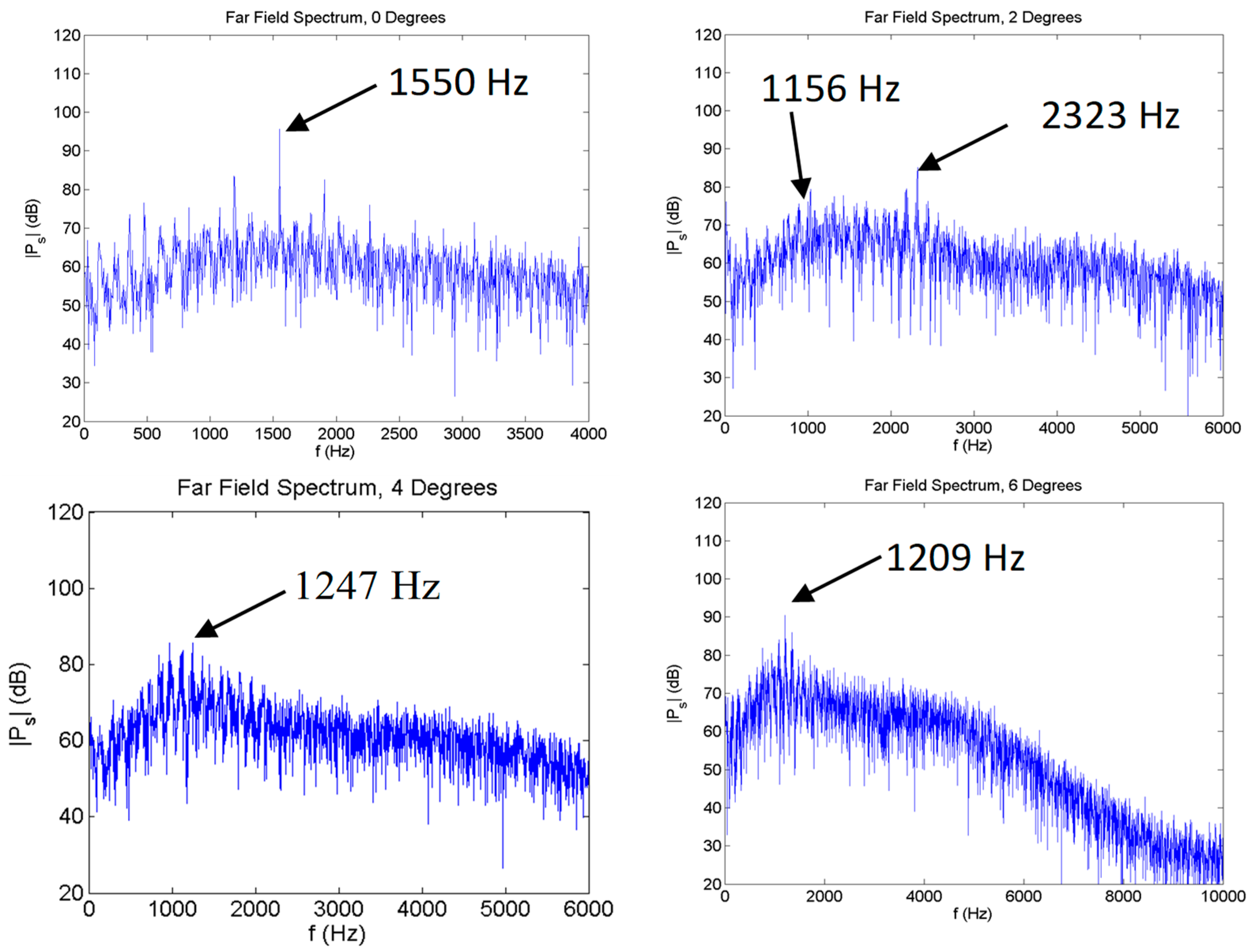
The presence of LSBs in these flow regimes, whether on the pressure or suction side, demonstrates the impact that LSBs have on triggering the AFL mechanism. In accordance with experimental observations of Lowson et al. [25], the tonal noise emission is clearly observed for the cases with α = 0°, 2°, 4°, and 6°, as seen in the acoustic spectra in Figure 7. Interestingly, all AoAs shown exhibit a single peak tone with the exception of the 2° case. The explanation for the dual tone can be tied to the formation of the LSB regions of Figure 6, which shows the 2° case to have an LSB on both the suction and pressure surface. To further investigate the roles of the airfoil suction and pressure surface LSBs in the mechanism of the airfoil tonal noise generation, LST is employed. 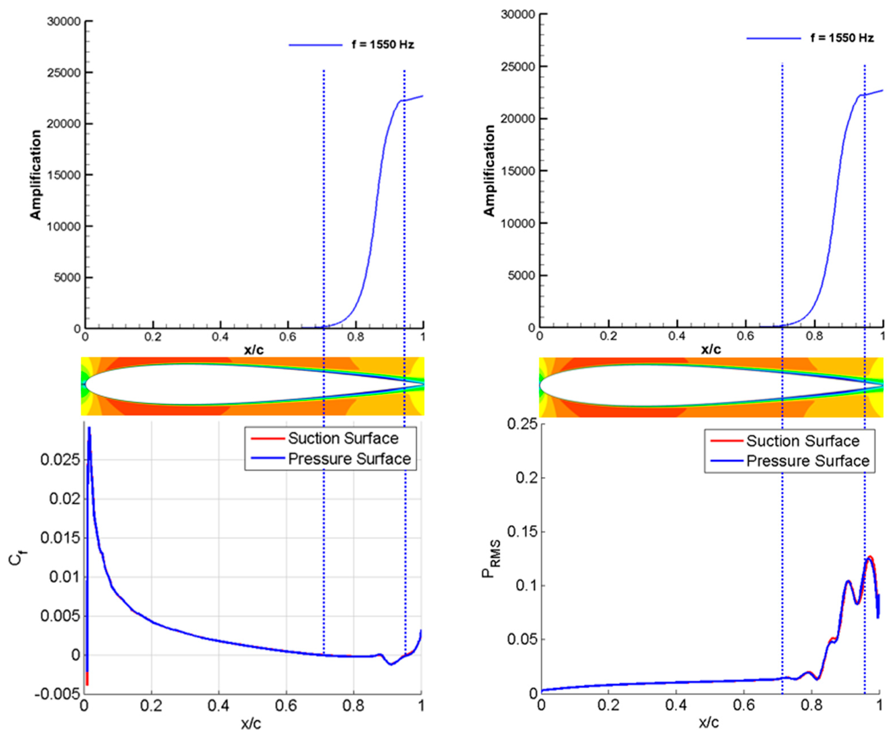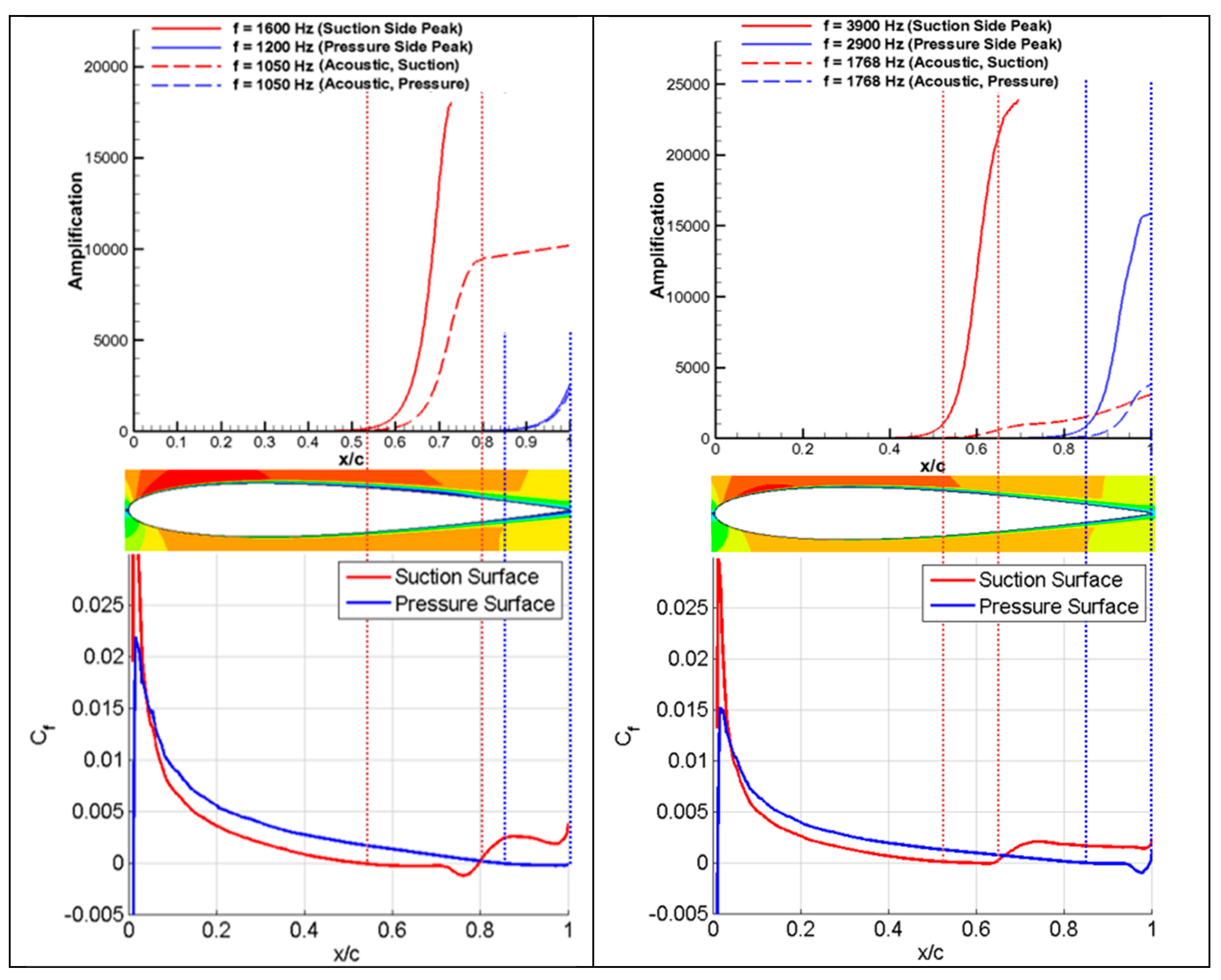For the α = 0° case, the linear stability analysis was conducted for frequencies ranging from 0 to 4000 Hz with increments of 10 Hz, as well as for the peak tonal frequency. Based on the symmetric nature of the configuration, only the data for the upper surface is presented in Figure 8. The primary region of instability growth prediction corresponds well with the location of the LSB, as indicated by the dashed blue lines revealing flow separation and reattachment locations determined from the coefficient of friction plot shown in the bottom. The accompanying velocity contours provides visual evidences of the existence of the LSB and correlates well with the instability growth.

To confirm the trends seen in Figure 8, data for α = 6° is obtained and presented in Figure 9. Based on the results tabulated in Table 3, only results for the suction side are shown due to the lack of LSB on the pressure side and the subsequent suppression of instability amplification. Additionally, the predicted modal amplification at the frequency of the acoustic tone is plotted for comparison. Although the peak frequency of 6375 Hz theoretically reaches a much higher amplification within the LSB, as predicted by the stability analysis (compared to the observed acoustic tonal peak of 1209 Hz), its growth quickly saturates at 20% chord with the flow reattachment, and the instability is likely to be damped out before reaching the TE. In contrast, the acoustic frequency mode, although significantly lower in amplitude, is sustained and grows in amplitude over the length of the airfoil.

Overall, the results clearly illustrate that the rapid growth of disturbances is associated with the LSB and the presence of the separation zone, which features an attached and separated region. In the attached regions, the instability waves develop as slowly-growing Tollmien–Schlichting (T-S) waves associated with the BL viscous effects. In the separated regions, the instability switches to the fast-growing Kelvin–Helmholtz (K-H) waves associated with the velocity gradients in the detached shear layers. This switch from T-S to K-H instabilities is critical and associated with the presence of the LSB and the ability of the convected mode to sustain the required amplitude before the instability mode is scattered into acoustic waves at the TE. 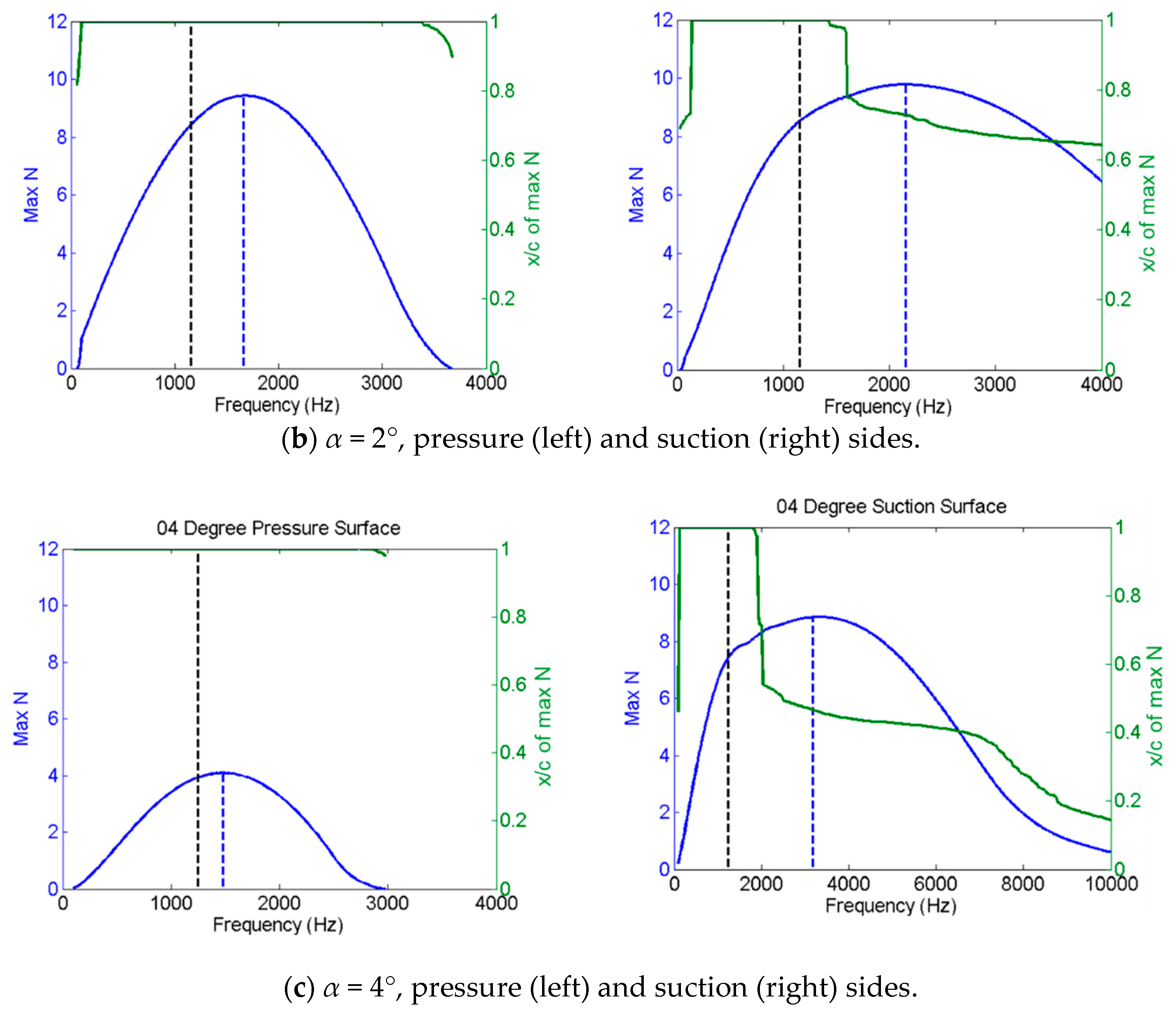For the considered range of the tone-producing AoAs, Figure 10 compares the LST-predicted frequencies corresponding to the instability waves with maximum amplification (dashed blue lines) against the peak frequencies of calculated acoustic spectra (dashed black lines). In addition, the solid green line is intended to indicate the airfoil surface location where each frequency mode reaches its maximum. Note that for α = 0°, the predicted frequency of the most amplified instability mode agrees well with the observed far-field frequency of 1550 Hz, showing a discrepancy of only 3.2%.

For other cases, however, a substantial difference is seen, and is also observed between the predicted peak amplifications on the suction and pressure surfaces. At α = 4°, the absence of the LSB on the pressure side of the airfoil results in weak instability growth, and similarly for α = 6° due to the favorable pressure gradient; thus, only the suction side is shown. Overall, these results are indicative of the increase in angle of incidence driving the discrepancy between the peak LST-predicted and acoustic tonal frequencies. Figure 11 supports this conclusion and shows the vortex shedding frequency agrees with the observed acoustic peak tone within 2% error at a low AoA. These results correspond to those of Jones et al. [26] and Jones and Sandberg [27] who performed their stability analysis based on DNS simulations of NACA-0012 airfoil at Re_c = 100,000 at 0° to 5° and found that the acoustic tone was identical to the vortex shedding frequency but was of lower frequency than the most amplified frequency predicted by LST. It should be noted that the tonal amplitudes are significantly higher on the suction surface, thus indicating instabilities on this side are the dominant source of pressure fluctuation growth shown earlier in Figure 8 and Figure 9.

Additionally, the fact that the LST-predicted peak instability tones may not be the ones radiating in the far-field as acoustics may be addressed using several arguments. On one side, LST predicts a certain frequency for maximum growth but in determining this peak frequency assumes that the initial amplitudes of all frequency components are identical. This peak amplitude thus could change if the initial level of the disturbance is not uniform and is a function of frequency. One may argue that the scattered acoustic waves, through the BL receptivity process, excite some frequency disturbances more than the others; this was elucidated by Jones et al. [26], who suggested that the BL receptivity process becomes increasingly more efficient at lower frequencies. Furthermore, while LST predicts a wide spectrum of rapidly-growing convected modes scattering at the TE into acoustic waves, the strength of the latter decreases with increasing frequency, as indicated by Jones and Sandberg [27] based on the application of Amiet’s TE noise theory [28]. Thus, one may expect that a particular low-frequency mode may be selected for optimum acoustic generation. Such a mode appears to be at the shedding frequency as it is naturally selected by the vorticity dynamics at the TE and its pattern of shedding into the wake. Another tone-selecting mechanism is the acoustic feedback determined by matching the phases of the acoustic and vortical modes. However, such mechanism described by the feedback-loop formula (further discussed below) produces many modes falling within the “unstable” category as determined by LST, and the fact that only a few of them are observed as primary peaks in the acoustic spectra appears to be solely determined by their proximity to the shedding tone. Indeed, the observed spectra indicate that the peak “cut-on” frequencies are the nearest to the shedding tone. This superposition also explains the dual-ladder tonal structure of Paterson et al. [1] since the scaling of the feedback-loop “cut-on” tone and the shedding tone is different with respect to the flow velocity.

Note that for the moderate Re_c laminar flow around a symmetric NACA-0012 airfoil, Tam and Ju [9] identified the shedding frequency with that of the most amplified near-wake K-H instability in the free shear layer. The TE scattering of such near-wake instability was claimed as the source of the shedding tone in the absence of AFL. Thus, such a wake instability mechanism may superimpose on the AFL mechanism of airfoil tonal noise production, with both related to the TE scattering of the free shear-layer K-H instabilities. This would point to the mutual resonance phenomenon where both mechanisms overlap and appear to enhance each other. When the flow past the airfoil is laminar with no AFL present, the remaining shedding tone appears at significantly lower amplitude, as demonstrated by Tam and Ju [9]. On the other hand, when the AFL mechanism is suppressed due to BL tripping or a low-intensity upstream turbulence, the observed acoustic spectrum still reveals a broadband hump centered around the shedding frequency (Golubev et al. [8]). It appears that the shedding mechanism is dominant and amplified with AFL presence due to the mutual interference and resonant interaction of the AFL-selected frequencies with shedding tone.

4.3. Variation in Angle of Attack for Re_c = 180,000: No Tone-Producing Regimes

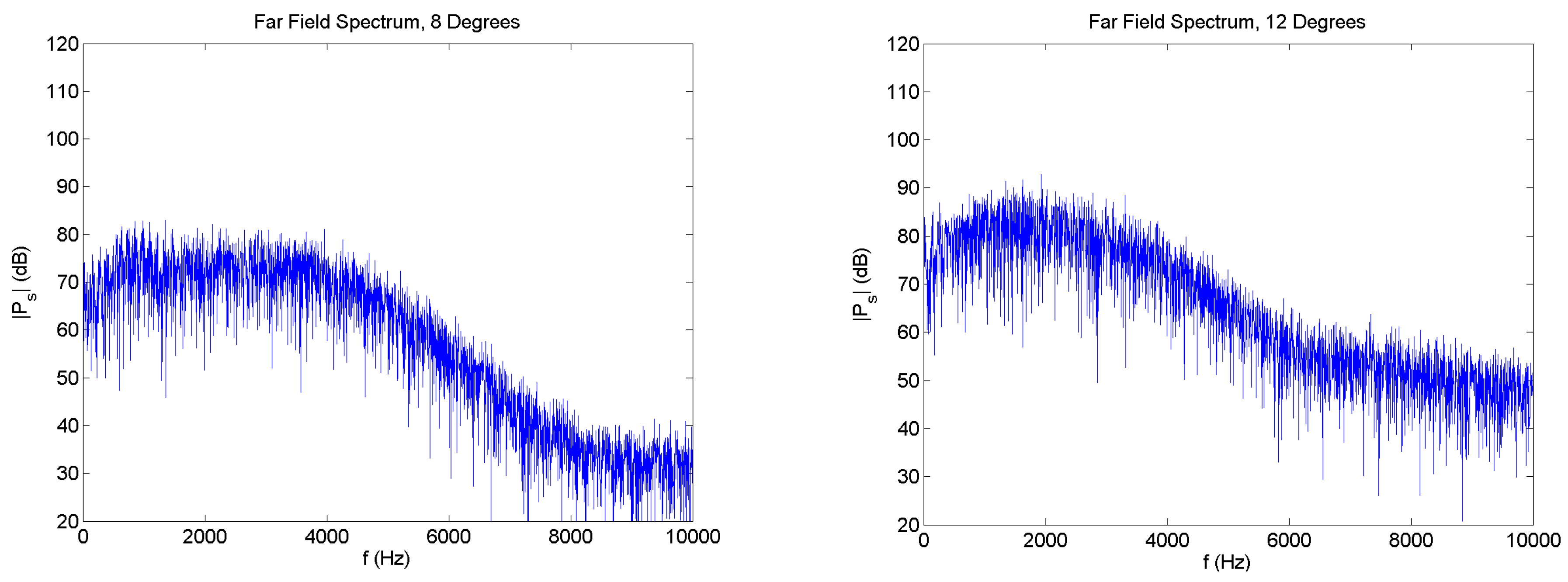
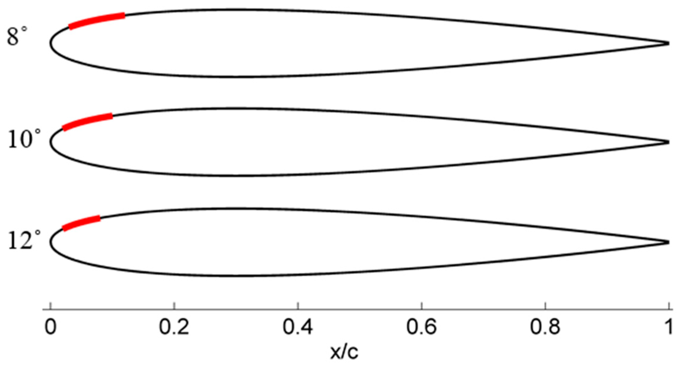
To investigate the effects at higher AoAs, the simulations were conducted for α = 8°, 10°, and 12°. Unlike the previous results, acoustic peaks are no longer present; thus, only spectra for 8° and 12° are shown (Figure 12). Separation regions that exists earlier at lower AoAs are no longer present on the pressure surface; however, the compact separation zones continue to persist near the LE on the suction surface, as shown in Figure 13 and indicated in

Table 4. LSB locations on the suction and pressure sides.

Angle	Suction Side	Pressure Side
8	3%–12%	-
10	2%–10%	-
12	2%–8%	-

based on the skin friction coefficient, C_f.

Result of the LST analysis (shown in Figure 14 for the α = 12° case) indicates that the separation regions near the LE provides the necessary condition to significantly amplify the high-frequency modes within the LSB. Nonetheless, these modes are quickly suppressed while the low-frequency counterparts continue to exist and grow mildly as they convect towards the TE. These results, however, may be influenced by 2D effects and are further discussed in the subsequent section.

Figure 15 shows the instantaneous vorticity contours for all three cases, illustrating the formation of vortical instability modes through the separation regions close to the LE. The orderly formation of vortices convecting to the TE at the tone-producing lower AoA is now substituted with a much less regular street of vortices, which barely graze the airfoil surface as they convect downstream. Furthermore, the emergence of small-scale turbulence forming near the LE points to the necessity for 3D ILES studies with higher-fidelity to properly resolve such flow regimes. Nevertheless, it may be hypothesized that due to the geometry of the flow at a high AoA, any remaining coherent vortical structures would lack the opportunity to strongly interact with the TE and thus would not scatter into the acoustic modes.

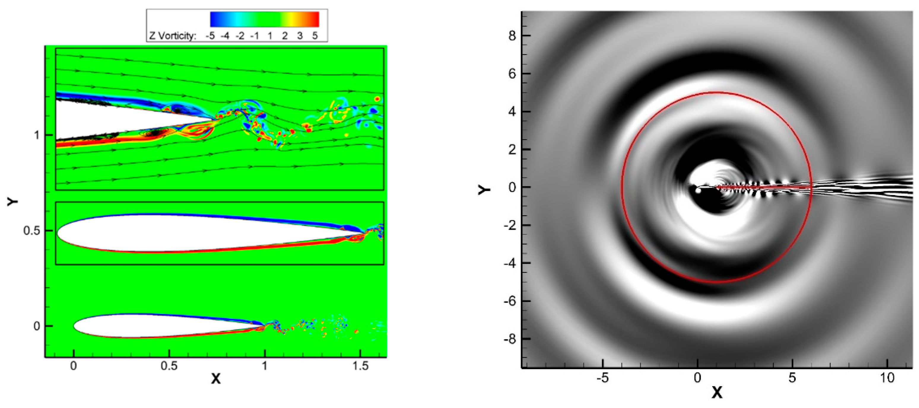
To test this hypothesis, full 3D ILES simulations (with grid dimensions shown in Table 1) were conducted for three cases at α = 0°, 4°, and 8°, with a fixed Re_c = 180,000, to elucidate the primary mechanism responsible for tonal noise suppression at an AoA greater than 6°. At α = 0°, shown in Figure 16, the flow remains in the transitional regime and its behavior is similar to that proposed by Brooks et al. [29]. Upon closer inspection of the Z-vorticity contours, the BL dynamics clearly reveals that the unsteady oscillatory motion of the vortex street at the TE is responsible for generating pressure pulses and the subsequent propagation of acoustic waves into the far-field. In addition to the vortex shedding noise, the interaction of the airfoil surface instabilities scattering into the wake is responsible for the additional noise contributions (neighboring peaks) shown in the surface spectra. The accompanying dilatation field shown in Figure 16 further confirms the acoustic wave to be emitted from the TE of the airfoil.

Increasing the AoA to α = 4° forces the suction-side BL transition point to move further upstream, resulting in a larger separation region, while the pressure-side BL does not separate. However, the flow regime is still classified as transitional. Z-vorticity contours in Figure 17 show coherent vortices and the resulting vortex shedding at the wake is still present. Therefore, it can be concluded that the mechanism responsible for the noise remains unchanged between the AoAs of 0° and 4°. The acoustic field shown in the instantaneous dilatation plot exhibits behavior similar to the α = 0° case and shows the noise source to originate at the TE.

As the AoA is further increased to α = 8°, the results illustrated in Figure 18 reveal that the flow has transitioned to a fully turbulent regime. Unlike the previous transitional regime, the vortical structures convecting along the surface and its subsequent vortex shedding in the wake are no longer coherent. Instead, the turbulent BL shows many small and random vortices to occur along the suction surface. This, along with the lack of strong vortex shedding, results in the suppression of the AFL and transforms the surface spectra to just a “broadband hump” near the natural shedding frequency. It should be noted, the noise generated by this regime still occurs at the TE as indicated by the dilatation field. This is mainly due to the interaction of the turbulent structures with the TE. In addition, the dilatation field shows the LE to radiate sound through the unsteady pressure fluctuations caused by the LE vortex. However, the high-frequency contributions are quickly suppressed and do not show up in the far-field. To ensure the LE contributions are not dissipated by an inadequate grid resolution, several checks were conducted at 0°, 90°, 180°, and 270°, and 360° around the LE, to confirm the wavelength of the pressure perturbations is accurately captured. The analysis revealed the frequency of the LE contributions to be approximately 2000 Hz, while the maximum resolvable frequency at those locations, based on the computational mesh, is approximately 3300 Hz. It is worth mentioning that the dilatation fields obtained from these three cases all show high amplitude contours in the wake region (between 5c and 10c), indicating the presence of hydrodynamic effects. However, the wake is steady in time and does not radiate any additional noise.

Results from the full 3D ILES reveal that the original hypothesis of the tonal noise suppression based on 2D simulations (suggesting the lack of coherent vortical structures interacting with the TE and scattering as acoustics) is, in fact, misleading. Instead, the actual 3D mechanism responsible for the AFL suppression at a high AoA is the transition to a fully turbulent flow regime with strong spanwise mixing.

4.4. Variation in Reynolds Number at α = 2°: Tone-Producing Regimes

To advance the understanding of the effect of flow velocity on tonal noise production, additional simulations were conducted for a range of Re_c at a fixed AoA of 2°. Clearly, all investigated cases are within the tone-producing region, and the cases of Re_c = 144,000 (20 m/s) and Re_c = 288,000 (40 m/s) selected for illustration exhibit well-defined tonal spectra in the near-field at 2 chords directly above the TE (Figure 19). BL statistical analysis reveals a direct correlation between increasing Re_c and the decreasing chordwise extent of the suction side LSB (Figure 20 and

Table 5. LSB locations on the suction and pressure sides.

Rec	Suction Side	Pressure Side
144,000	52%c–80%c	84%c–100%c
180,000	53%c–74%c	82%c–100%c
216,000	54%c–69%c	80%c–100%c
252,000	55%c–66%c	82%c–100%c
288,000	57%c–64%c	85%c–100%c

), while the LSB on the pressure surface retains nearly the same size at the TE (with C_f becoming more negative towards the TE with increasing velocity).

Correspondingly, the LST results demonstrate that an increase in Re_c leads to a surge in amplification of the peak instability mode on the airfoil pressure side (Figure 21). At the same time, as the suction-side LSB shrinks while the instability saturation location shifts further upstream from the TE, the contribution of the suction surface to the radiated sound diminishes relative to that from the pressure side. It is expected that a further increase in flow velocity will result in the eventual suppression of the separation region from the suction side. When this occurs, the pressure-side LSB will provide the sole contributor to the radiated tonal noise. These trends are in agreement with the experimental findings of Golubev et al. [8], Yakhina et al. [10], and Pröbsting et al. [30], where tripping the BL on either side of the airfoil revealed a dominant tonal noise contribution from the suction side at the lower flow velocities, and from the pressure side at the higher flow velocities.

Further extension of the flow regime towards a lower Re_c (<144,000) would lead to the formation of a fully laminar BL and result in the absence of the LSB. Consequently, without the LSB, the switch from T-S to K-H waves would not be possible and thus the rapidly amplifying instability modes needed for the self-sustained acoustic feedback can never be established. While it is possible for the shedding tone to still exist, it would likely be much lower in amplitude due to the lack of reinforcement from the feedback loop [9]. On the other hand, increasing the Re_c (>288,000) would suggest transitioning to the fully turbulent BL flow, with both the acoustic feedback and the shedding tone fully suppressed.

4.5. Acoustic Radiation Frequency Structure

Arbey and Bataille [3] suggests that a transitional airfoil emitting tonal noise is the result of two mechanisms: the first is the scattering of vortices along the airfoil surface into the wake at the airfoil TE, and the second is the natural vortex shedding. The current section focuses on investigating the BL dynamics of the airfoil surface to examine the instability point of inception and the subsequent behavior of the flow. To achieve this task, the effect of mean flow velocity (

Table 6. Mean flow condition.

U∞ (m/s), Rec
16 (128,000), 19 (152,000), 21 (168,000), 25 (200,000)

) is further analyzed from the previous section to establish a connection between the LSB and its effect on the AFL. The selected cases correspond to an airfoil with the chord c = 0.12 m installed at the geometric AoA of 0°, closely representing the experimental conditions of Yakhina et al. [10,31].

Figure 22a illustrates the Z-vorticity contours of an airfoil subjected to a 16 m/s (Re_c = 128,000) uniform upstream flow, revealing the expected vortex roll up and shedding pattern. As described by Arbey and Bataille [3], the onset of instabilities occur at 0.86c due to the T-S waves that grow and transition to discrete vortices, which convect along the airfoil surface towards the TE. Once the vortices reach the TE, their interaction with the natural shedding of the wake coalesce to amplify the noise generated by the airfoil. As the mean flow velocity is increased to 19 m/s (Re_c = 152,000) (Figure 22b), the overall behavior of the flow remains unchanged with the exception of the triggering of T-S to K-H instabilities. Unlike the 16 m/s (Re_c = 128,000) case, at 19 m/s (Re_c = 152,000), the transition from T-S to K-H instabilities appears further upstream as the increase in the flow velocity shifts the location of the separation region towards the LE. A similar pattern is exhibited as the mean flow velocity is increased to 21 m/s (Re_c = 168,000) (Figure 22c) and 25 m/s (Re_c = 200,000) (Figure 22d). It is worth mentioning that for all the flow regimes shown in Figure 22, the LSB is present and is the primary source to trigger instability amplification and the sustainment of the AFL.

To further demonstrate the effect of Re_c on the tonal noise mechanism, spectral analysis is employed for various experimental probe locations along the airfoil surface (shown in Figure 1) to obtain the peak and neighboring tones. Details of the Fourier analysis performed to obtain the spectra are similar to those employed in the previous sections. However, for all subsequent near-field (2c above TE) spectra in this chapter, the results were obtained by sampling a signal that was 5 times longer, thus allowing for averaging of the FFT (using 5 segments) to smooth out the noise and accentuate the peaks of the signal. 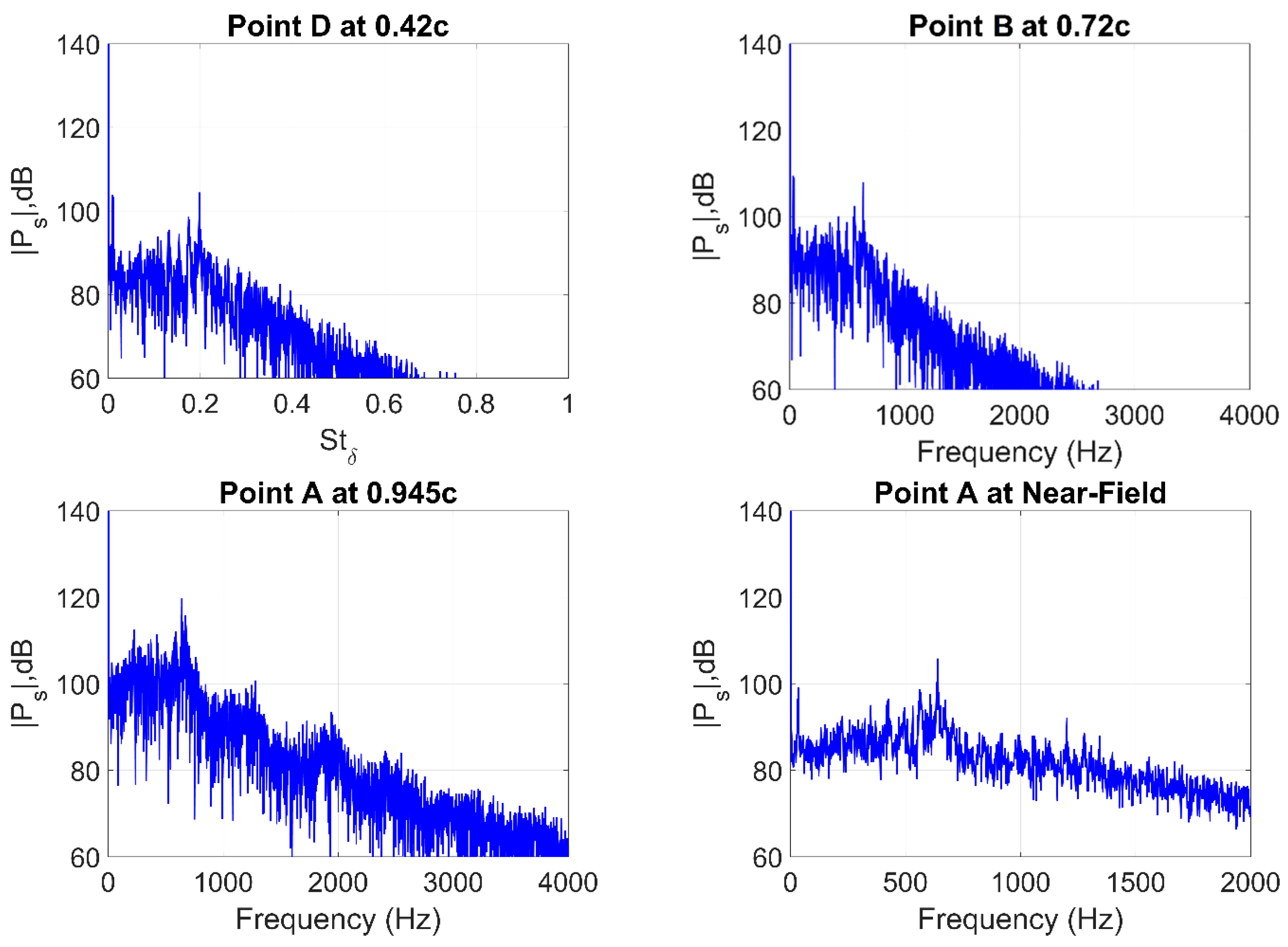Figure 23 reveals the peak tonal noise (corresponding to Strouhal number St ~0.2) predicted by the numerical simulations for the mean flow velocity of 16 m/s (Re_c = 128,000) to occur at a frequency of 636 Hz for every selected point along the airfoil, which correlates well with Paterson’s [1] empirical formula (14) for vortex shedding frequency,

$$f_s=\frac{0.011U_{\infty }^{1.5}}{{\left(Cv\right)}^{1/2}}$$

(14)

where c is the airfoil chord and ν is the flow kinematic viscosity. Although the neighboring tones are more difficult to distinguish due to the low amplitudes, the equally distant spaced peaks, $\mathsf{\Delta }f$, are indicative of their existence. Furthermore, the peak amplitude of 120 db is revealed to occur at point A (0.945c) close to the TE, with the amplitude decreasing for upstream probes. This behavior confirms that the main noise source is, in fact, located at the TE where the scattering takes place.

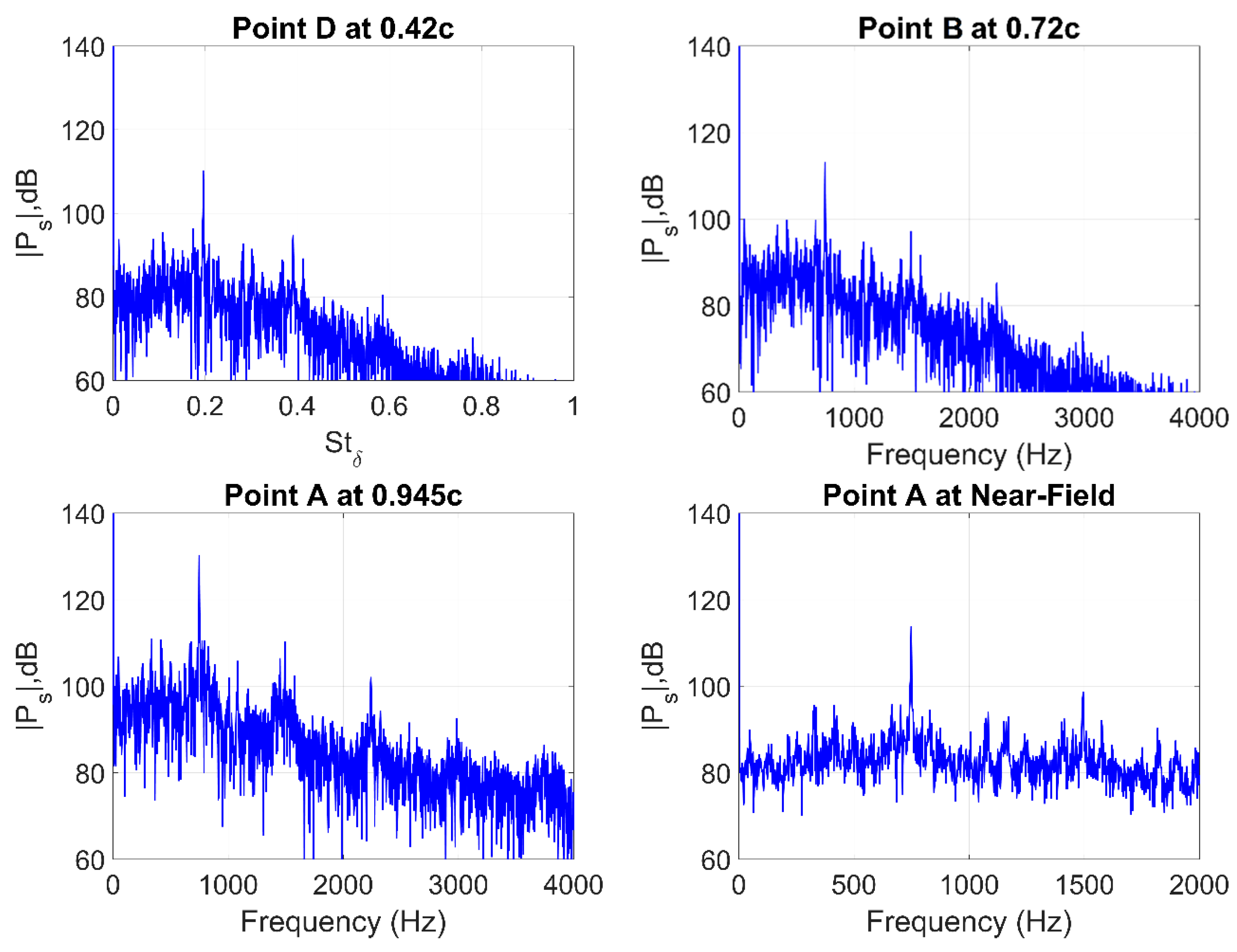
As the mean flow velocity is increased to 19 m/s (Re_c = 152,000) (Figure 24), the peak tone shifts rightward in the spectrum and occurs at a higher frequency of 746 Hz (while maintaining St ~0.2). Again, correlating this value with Paterson’s formula (14) provides a good match and reveals that the increase from 16 m/s (Re_c = 128,000) to 19 m/s (Re_c = 152,000) would result in a shift from 574 Hz to 729 Hz. This confirms that the peak tones do in fact scale with ~U^1.5, thus corresponding to the airfoil’s natural shedding frequency. Additionally, the increase in the flow velocity leads to neighboring tones with higher amplitudes that are more prominent and easily distinguished in the spectrum. Further increase in mean flow velocity to 21 m/s (Re_c = 168,000) and 25 m/s (Re_c = 200,000) shows a similar trend. Figure 25 and Figure 26 demonstrate the shift of the primary tones to higher frequencies, in agreement with Paterson’s formula (14).

Overall, all the considered cases exhibit a similar trend, with the spectral pressure levels peaking at the TE. On the other hand, the case of 25 m/s (Re_c = 200,000) (Figure 26) reveals that while the highest amplitude tone is observed at point A at 1199 Hz, correlating well with shedding frequency (14), and the probes at points B, C, and D show a peak tone at 1281 Hz. As suggested based on the LST analysis, this could be linked to the amplification of various instability modes occurring along the airfoil surface. Perhaps the peak shedding tone of 1199 Hz observed at the TE reduces in amplitude as it propagates upstream and interacts with probes B, C, and D. At the same time, it could be that the secondary peak of 1281 Hz results from a mode that is more amplified in the regions close to points B, C, and D but appears weaker at the TE, where the interaction of the saturated instability modes with the primary shedding mechanism dominates.

It is also worth noting that increasing the flow velocity from 16 m/s (Re_c = 128,000) to 25 m/s (Re_c = 200,000) directly affects the amplitudes of the neighboring tones surrounding the peak, and as a result, leads to a very pronounced peak. This comparison is clearly illustrated in Figure 24 and Figure 26 in which the former shows a very low amplitude with nearly suppressed neighboring tones, while the latter shows clearly defined tones. This observation correlates well with the Z-vorticity contours in Figure 22 by visually inspecting the vortices scattering in the wake and correlating the amplification of the neighboring tones with the amplitudes of the vortical structures developing along the airfoil surface. It is evident that at 16 m/s (Re_c = 128,000) the vorticity contours are not as saturated compared to 25 m/s (Re_c = 200,000), which is indicative of stronger vortex cores. These stronger vortex cores will, in turn, produce stronger acoustic waves and thus show higher amplitudes of the predicted spectral peaks.

Results obtained from the spectral analysis are now analyzed in order to reconstruct the ladder-type tonal frequency structure originally obtained by Paterson et al. [1].

Figure 27 shows such a reconstruction using the numerical data presented in Figure 23, Figure 24, Figure 25 and Figure 26, in comparison with the shedding-tone formula (14) and experimental results of Yakhina et al. [31]. Note that f_s is graphically determined by selecting a single highest amplitude peak tone recorded at the four monitor points along the airfoil (typically at the TE). The remaining neighboring tones, f_n, are obtained by selecting the equally spaced tones surrounding the peak tone. The reconstructed ladder structure demonstrates that the solid line, f_s, follows Paterson’s proposed U^1.5 and f_n, dashed lines, follows the U^0.8 scaling. The agreement between Paterson’s formula (14) and the ILES results correlate very well and verifies the accuracy of the current numerical results as well as the existence of the AFL.

To further validate the existence of the AFL at these flow regimes, a dispersion curve analysis (Smith et al. [32], 2012) was employed to predict the convective flow velocity (U_c) along the airfoil surface, which can be used in the feedback-loop formula of Arbey and Bataille [3],

$$\frac{f_{n}L}{U_c}\left(1+\frac{U_c}{a_0-U}\right)=n+\frac{1}{2}$$

(15)

where L is the distance from the point of maximum surface velocity to the TE and $a_0$ is the speed of sound. With these terms defined, Equation (15) can be rearranged to provide the AFL-selected modes (n) and match with the predicted ones.

The results presented in Figure 28 are obtained using 2¹⁴ pressure slices extracted from the airfoil surface near the TE (0.85c–0.95c) over a period of 0.487 s to show a 2D spectrum representing the normalized frequency fδ/U_∞ vs. the normalized wavenumber, k_xδ/2π, where δ is the BL thickness. The selected flow region, measuring 0.1c × 0.03c, was chosen to be near the TE based on the dilatation field revealing the TE to be the primary source of the airfoil acoustic radiation.

Table 7. Computed (CFD) vs. predicted (Equation (15)) tonal frequencies.

16 m/s (128,000)					19 m/s (152,000)
f, Hz computed (CFD)	562	640	720		f, Hz computed (CFD)	633	746	835
	n = 10	n = 12	n = 13			n = 10	n = 11	n = 12
f, Hz predicted, Equation (15)	557	663	716		f, Hz predicted, Equation (15)	700	766	833
21 m/s (168,000)					25 m/s (200,000)
f, Hz computed (CFD)	699	820	939		f, Hz computed (CFD)	963	1099	1218
	n = 8	n = 10	n = 11			n = 9	n = 10	n = 11
f, Hz predicted, Equation (15)	696	860	942		f, Hz predicted, Equation (15)	992	1097	1202

compares the computed (from numerical analysis) vs. predicted (Equation (15)) tonal frequencies for the four cases from 16 m/s to 25 m/s, to show a good agreement for the selected modal numbers. The remaining discrepancies are attributed to the change in the convective velocity along the airfoil surface not accounted in the employed Equation (15).

5. Discussion of Results

High-accuracy 2D and high-fidelity 3D (ILES) numerical experiments were conducted to investigate the phenomena related to flow-acoustic resonant interactions at moderate Reynolds numbers characteristic of transitional airfoils. Numerical analyses were employed to examine the airfoil BL dynamics, including the statistical moments and surface pressure spectra, as well as the airfoil acoustic radiation in the far-field.

The first part of the study focused on thorough validation of the numerical model by comparing the unsteady responses of the NACA-0012 airfoil for selected flow regimes against the experimental data of Yakhina et al. [10]. The results indicate that 2D and 3D ILES predictions compare well with experimental data. In particular, the conducted far-field spectral analysis showed a near perfect match of computational and experimental results at frequencies surrounding the peak tones. The predicted near field showed a good match of the tonal content but elevated broadband levels resulting from the unsteady hydrodynamic fluctuations that do not propagate into the far field. In addition, the similarities observed between the 2D and 3D ILES predictions vs. experimental data allowed the majority of the numerical experiments to be conducted using the 2D approach.

The transition between the tone-producing and no-tone-producing flow regimes was thoroughly investigated for the NACA-0012 airfoil at a different AoA and Re_c and correlated with position and size of the LSB. At low AoAs (α ≤ 6°), distinct tones were shown to be present that dominated the acoustics of the airfoil. However, the tones disappeared at higher AoAs (α > 6°) due to the LSB migration towards the LE, which allowed sufficient time for the flow to transition to fully turbulent regime with subdued AFL interactions. On the other hand, for a fixed AoA, the increase in flow Re_c was associated with LSB shrinking on the suction side and an increasingly dominant contribution of the AFL on the pressure side to the tonal noise production. Additionally, a parametric investigation of the effect of Re_c allowed recreating Paterson’s dual ladder-type frequency structure. Overall, the results of the parametric studies involving high-fidelity numerical studies and linear stability analysis clearly demonstrate that the rapid growth of the BL instability modes is associated with the presence of separation regions (i.e., LSB) on either side of the airfoil. The switch from the slowly growing T-S modes (associated with the BL viscous effects) to the fast-growing K-H modes (associated with the velocity gradients in the LSB detached shear layer) thus appears as a necessary condition for the strong multiple-tone-producing flow-acoustic interactions. This allows for an important modification to the AFL scenario originally proposed by Longhouse [33], as illustrated in Figure 29. The additionally required condition is the ability of the vorticity modes to sustain their presence and sufficient amplitude to the TE for the effective acoustic scattering process to take place. Hence, the LSB must be located close enough to the airfoil TE to prevent the subsequent destruction of the saturated coherent modes (rollers) through turbulent BL transition and spanwise mixing process.

Finally, the AFL frequency selection mechanism was addressed. It was noted that, for a low Re_c laminar flow around a symmetric NACA-0012 airfoil, Tam and Ju [9] identified the shedding frequency with that of the most amplified near-wake K-H instability in the free shear layer. The TE scattering of such near-wake instability was claimed as the source of the shedding tone in the absence of AFL. It is plausible that such a wake instability mechanism may superimpose on the AFL mechanism of airfoil tonal noise production, with both related to the TE scattering of the nonlinearly saturated K-H modes. This points to the mutual resonant interaction wherein both mechanisms overlap and appear to enhance each other. To this end, when the airfoil flow is laminar with no AFL present, the remaining shedding tone appears at a significantly lower amplitude, as demonstrated by Tam and Ju [9]. On the other hand, when the AFL mechanism is suppressed due to BL tripping or a low-intensity upstream turbulence, the observed acoustic spectrum still reveals a broadband hump centered around the shedding frequency. It thus appears that the naturally primary shedding mechanism is dominant and amplified by the AFL presence due to the mutual interference and resonant interaction of the AFL-selected frequencies with the shedding tone. The latter essentially elevates that part of the spectrum of the amplified BL instability modes that appears the closest to the shedding tone. This may explain the divergence between the frequencies of the most amplified instability modes and the acoustically radiated peak tone coinciding with the shedding frequency. It is the interaction of the two mechanisms that produce the dual ladder-type acoustic tonal structure of Paterson et al. [1], with multiple AFL-selected tones staged around the shedding tone.