Abstract
Incremental learning is a methodology that continuously uses the sequential input data to extend the existing network’s knowledge. The layer sharing algorithm is one of the representative methods which leverages general knowledge by sharing some initial layers of the existing network. To determine the performance of the incremental network, it is critical to estimate how much the initial convolutional layers in the existing network can be shared as the fixed feature extractors. However, the existing algorithm selects the sharing configuration through improper optimization strategy but a brute force manner such as searching for all possible sharing layers case. This is a non-convex and non-differential problem. Accordingly, this can not be solved using powerful optimization techniques such as the gradient descent algorithm or other convex optimization problem, and it leads to high computational complexity. To solve this problem, we firstly define this as a discrete combinatorial optimization problem, and propose a novel efficient incremental learning algorithm-based Bayesian optimization, which guarantees the global convergence in a non-convex and non-differential optimization. Additionally, our proposed algorithm can adaptively find the optimal number of sharing layers via adjusting the threshold accuracy parameter in the proposed loss function. With the proposed method, the global optimal sharing layer can be found in only six or eight iterations without searching for all possible layer cases. Hence, the proposed method can find the global optimal sharing layers by utilizing Bayesian optimization, which achieves both high combined accuracy and low computational complexity.
1. Introduction
Recently, computer vision technologies, including image recognition and object detection, have developed rapidly in the field of deep learning [1,2]. Despite these remarkable achievements, one of the significant challenges in neural network-based computer vision algorithms is learning new tasks continually, like the cognitive process of human learning [3,4,5]. Because in practical situations, new datasets for new tasks are obtained in an incremental manner, meaning that the network only accesses the dataset for new tasks [6]. Three conditions are needed for the successful incremental learning algorithm:
- i
- The subsequent data from new tasks should be trainable and be accommodated incrementally without forgetting any knowledge in old tasks, i.e., it should not suffer from catastrophic forgetting [7].
- ii
- The overhead of incremental training should be minimal.
- iii
- The previously seen data of old task should not be accessible when it is training incrementally.
For incremental learning, most of previous works have focused on utilizing knowledge acquired from previously learned tasks and transferring them to a new task, avoiding “catastrophic forgetting” [8,9,10]. Li and Hoiem [11] proposed ‘Learning without Forgetting (LWF)’ to exploit knowledge distillation [12] as a solution to catastrophic forgetting. Using only datasets for the new tasks, they encourage reducing the variance between the output probabilities of old classes in the original network and that in the updated new network. In addition, Michieli et al. [13] proposed incremental learning for sementic segmentation, while previous works focused on only object detection or classification problems. This methodology introduced four types of knowledge distillation strategies such as knowledge distilled on the output layer, on the intermediate feature spaces, on dilation layers, and on the intermediate layers of the decoding. They also tried to freeze only the first couple of convolutional layers allowing to preserve the lower level descriptions. However, this method only freezes the first couple of convolutional layers, rather than considering how much layer can be shared to preserve the feature extraction capabilities unchanged from previously learned task. Nguyen et al. [12] introduced a methodology to select how much convolutional layers can be shared for incremental learning by considering where the forgetting issue comes from. There are two steps of the methodology, which are ‘Catastrophic Forgetting Dissector (CFD)’ and ‘Critical Freezing’ approaches. The first step is to explain how forgetting happens, based on the vision network models to figure out the most flexible convolutional blocks in a network, and the second step is to freeze weights of the earlier blocks than the most flexible convolutional layers. However, although the relationship between the accuracy and the ratio of freezing weights is a trade-off to be balanced, this methodology is limited to find the most flexible convolutional blocks adaptively with given requirements. Sarwar et al. [14] focused on hardware and energy requirements for model update [15,16,17], then proposed a ‘clone-and-branch’ technique leveraging general knowledge from previous tasks to learn subsequent new tasks by sharing some initial convolutional layers of the base network as fixed extractors and fine-tuning in the new branch. This is because a deep convolutional neural network (DCNN) denotes the neural network that consists of multiple convolutional layers to extract hierarchical visual features [9,18]. Thus, when the image is fed into a DCNN, the network transforms the image hierarchically layer by layer. Observing features learned by a convolutional neural network, the earlier convolutional layers extract basic features like color and texture, while the later layers extract more detailed and sophisticated features like certain parts of objects [19,20,21]. Hence, in [14], they identify to determine how much of the initial convolutional layers in the base network for learning new classes having similar features as the classes in the base network. However, estimating optimal sharing layer configuration is a non-convex and non-differential problem, so it cannot be solved using the gradient descent algorithm or convex optimization method [5,22,23]. Therefore, this method should explore all possible sharing layer cases to find the optimal ones that meet quality specifications and approximate the existing network sharing capacity for the new task-specific sharing configuration via similarity score. Thus, it forces to high computation complexity [24]. To solve this limitation, the proposed method utilizes a Bayesian optimization technique (BayesOpt) to get the optimal number of sharing layer without considering all possible cases. The BayesOpt is a class of machine learning-based optimization algorithm, and there are several previous works that shows BayesOpt guarantees the global convergence in combinatorial optimization problem [25,26]. Therefore, with a properly designed loss function, the proposed algorithm can find a global optimal sharing layer for layer sharing-based incremental learning.
In summary, the contributions of the proposed method are as follows:
- We firstly define the sharing layer ratio estimation problem for incremental learning as discrete combinatorial optimization problem with the global optimization strategy.
- By utilizing BayesOpt, the proposed method effectively computes the global optimal sharing capacity of the existing network for accommodating the new task without computing all possible cases.
- The proposed algorithm can adaptively find the global optimal sharing configuration with the target accuracy via adjusting the threshold accuracy parameter in the proposed loss function.
- To employ BayesOpt, the proposed objective function should be continuous. It is a discrete function due to the number of layers, designed to represent the continuous combinatorial optimization problem with a step function.
The remainder of this paper is organized as follows. Section 2 gives the brief explanations of target incremental learning algorithm in [14]. Section 3 introduces our proposed algorithm focusing on both the proposed objective function and the utilization of BayesOpt. Section 4 shows the experimental results on the representative classification dataset. Finally, Section 5 summarizes the proposed algorithm. This work is an extension version of [27].
2. Preliminaries
In this section, we briefly describe the ‘clone-and-branch’ technique in [14] which we target, and define the problems in the existing method.
2.1. Incremental Learning Algorithm Based on ‘Clone-and-Branch’
A deep convolutional neural network (DCNN) denotes a neural network that consists of multiple convolutional layers to extract hierarchical visual features [9,18]. By tracking the feature projection to these convolutional layers, the earlier layers extract the most basic part of an image, i.e., edges, colors, and textures, while the later layers extract much more detailed and sophisticated structures [19,20,21]. For efficient incremental learning, ref. [14] proposed a training methodology called the ‘clone-and-branch’ technique, depicted in Figure 1. This method leverages general knowledge from previously learned tasks to learn subsequent new tasks by sharing initial convolutional layers of base networks. The basic idea is that the earlier layer of base network can be used for learning new task, especially in a similar domain of input used in new task [8,9]. Besides, when the branch network is in training, the last convolutional layers of the base network remain disconnected, so that the network can learn new tasks one after another without any performance loss in the knowledge of the base network. In ‘clone and branch’ technique, there are two steps of training methodology, which consist of both empirical searching method and similarity scoring method.
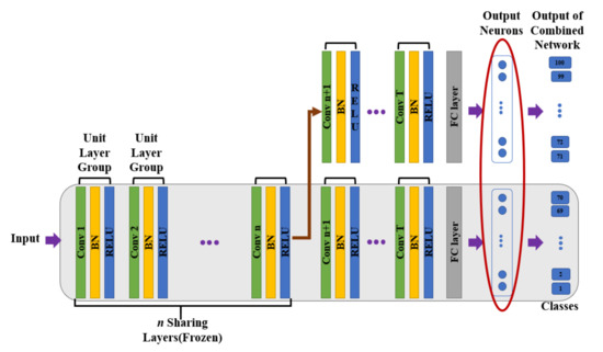
Figure 1.
The incremental network structure called ‘clone and branch’. The shaded gray rectangle is the base network. Each time we update the network for the new task, some initial parts of convolutional layers are shared and frozen, so only the branch part of layers is retrained with the new task data, while the last layers of the base network remain disconnected.
2.1.1. Step 1: Empirical Searching
In order to select optimal sharing layer number for learning new tasks, they generate an ‘accuracy vs. sharing’ trade-off curve. Through this trade-off curve, we can observe the fewer earlier layers are used to share, the better the inference performance of the branch network, since the layers in a large DCNN can extract more detailed features of specific tasks as going up to the upper level. On the other hands, if they share more than a certain ratio of the network parameters, a drastic accuracy drop can be observed. Thus, this curve allows to determine the optimal sharing configurations without severe accuracy degradation on new task. However, there is a large overhead for determining the optimal sharing configuration that meets quality specifications from this curve. Because for generating an ‘accuracy vs. sharing’ trade-off curve, they need to utilize only a brute force manner such as searching for all possible sharing layer cases. This is because the problem of estimating the optimal sharing layer number is a non-convex and non-differential problem, so they cannot be solved by using powerful optimization techniques such as the gradient descent algorithm or other convex optimization strategies, and it leads to high computational complexity.
2.1.2. Step 2: Utilizing Similarity Score
To get the sharing capacity of the base network for each new-task, a similarity score is utilized. For generating a similarity score, few random samples of each class in a new task are passed through the pre-trained base network. From the classification results, they assume that the number of repeating classes is regarded as a similarity score, which is approximately quantified the similarity between the classes of the base network and the new task. This is because if same classification results repeatedly appear in classes of a new task as in some specific classes of the base network, it can be considered that feature representation of new classes is similar to that of specific classes in the base network. However, utilizing the similarity score is not accurate or ideal. Because it can not be robust on few randomly sampled data, the similarity score essentially has approximation errors on accuracy degradation in incremental learning.
2.1.3. Problem Definition
Based on what was explained in the prior subsection, ‘clone-and-branch’ optimizes the objective function as follows:
where is the approximate sharing configuration of the base network at the ‘accuracy vs sharing’ trade-off curve, is the similarity score between new tasks and the base network, and is the similarity score between specific new task ‘n’ and the base network. Then, is the optimal sharing configurations of base network for accommodating a new task ‘n’. As shown in Equation (1), the problem to select the number of global optimal sharing layers for learning new tasks is non-convex and non-differential which is difficult to be solved by using a proper optimization strategy. To solve this issue, we firstly define this as a discrete combinatorial optimization problem and propose a novel efficient incremental learning algorithm-based Bayesian optimization which guarantees the global convergence even though the problem is non-convex and non-differential. The proposed method will be described in more detail in the following sections.
3. Proposed Algorithm
In this section, we explain both the proposed objective function for selecting optimal sharing layer and optimization details of the proposed algorithm through BayesOpt.
3.1. Combined Classification Accuracy
The combined classification accuracy measures the quality of incremental learning with n initial sharing layers by activating the combined softmax of both the base network and the new branch network simultaneously. The equation of the combined classification accuracy is as follows:
where N denotes the total number of data for testing combined classification, is the ith data for testing, is the label of , and denotes accuracy on , respectively. Therefore, if the output of the combined network has the same value with the ground truth on . i.e., , it provides 1 or otherwise 0.
3.2. Target Combined Classification Accuracy
In our proposed algorithm, there is the target combined classification accuracy, which should meet some degraded accuracy within the baseline as the required quality specification. The baseline is the combined classification accuracy without any sharing layer of the base network.
where is the baseline and is the threshold accuracy degradation value. Then, is the target combined classification accuracy. The reason of utilizing to define is that is the upper-bound value of accuracy, where every layer of the network is updated for new tasks without any network sharing.
3.3. Proposed Objective Function
The objective function with sharing some of the initial convolutional layers n is the linear-combination between and . The is the global optimal configurations for the target combined classification accuracy degradation in the incremental learning modeling, and it minimizes the objective function. Hence, the objective function is as follows:
However, as selecting the number of global optimal sharing layers in the discrete optimization problem, the objective function has the form of a discrete function. This form can not be applied to BayesOpt, because the BayesOpt guarantees the global convergence in continuous but the non-derivative combinatorial optimization problem. To solve this problem, we change the proposed objective function in a continuous step function. Therefore, even though the modified objective function is not differential, it can be solved by BayesOpt. In other words, it is possible to find the optimal global rank via the proposed objective function.
3.4. Global Optimal Layer Selection via BayesOpt
In the proposed algorithm, the optimal number of sharing layer is found through BayesOpt which enables to optimize an objective function, globally. The BayesOpt consists of two major components: (1) Gaussian process (GP) regression, which statistically defines the uncertainty of an objective function, (2) an acquisition function which selects where to sample next [28,29]. The GP regression provides a Bayesian posterior probability distribution of the proposed objective function, which denotes potential value of at an unidentified number of sharing layer n. After the GP regression, the acquisition function measures the value which would be evaluated for next optimization iteration, in other words, it decides the best candidate n which induces better objective function value than previously computed points. In the following sections, we discuss the components of BayesOpt in detail, first explaining GP regression and describing acquisition functions including probability improvement (PI) and expected improvement (EI).
3.4.1. Gaussian Process (GP) Regression
GP regression is a Bayesian statistical approach for modeling an objective function [29]. Just as Gaussian distribution is a distribution over a random variable, completely specified by its mean and covariance, GP regression is a distribution over objective functions, identified by its mean function and covariance function. Any finite set of k points in n, produces a k-dimensional Gaussian distribution on , taken to be a distribution on . GP regression considers this k-dimensional Gaussian distribution as the prior distribution with a mean vector and covariance matrix . The resulting prior distribution on is defined as follows:
where means a vector which is constructed by evaluating a mean function at each in , denotes the covariance matrix which is composed by evaluating a covariance function at each pair of points , in . In GP regression, the covariance function should produce large positive correlation when and are closer in the input space.
From the above prior distribution, the conditional distribution of can be computed by Bayesian rule.
where is
and is
This conditional distribution is called a posterior probability distribution and quantifies the uncertainty of loss function value on the unidentified sharing layer points n.
The performance of GP regression to represent a valuable distribution on the objective function depends on the covariance function. Therefore, in the proposed algorithm, we utilize automatic relevance determination (ARD) Màtern 5/2 function as a covariance function:
where is , and are hyper-parameters. This covariance function results in twice differentiable sample functions, a hypothesis that corresponds to those made by, quasi-Newton methods, but without requiring the smoothness of the squared exponential.
3.4.2. Probability of Improvement (PI)
After the GP regression, the acquisition function determines which point in the input space should be evaluated next via proxy optimization:
where denotes the acquisition function.
One intuitive approach is to maximize the probability of improving the best current point , which is called as “probability of improvement (PI)”. Under the GP regression, the PI can be calculated as:
where is
and denotes the cumulative distribution function of the standard normal distribution.
The drawback of PI is that this strategy is based on pure exploitation. Points that have a high probability of being smaller than will be drawn over points that offer larger gain but less certainty [28,29,30].
3.4.3. Expected Improvement (EI)
To mitigate the limitations of PI, the proposed algorithm uses an expected improvement (EI) acquisition function to decide the next observation points [28,31].
where denotes the standard normal density function.
The EI concerns the predictive distribution of GP regressions to balance the trade-off of exploiting and exploring [28,29,30,31]. In other words, when exploring, EI determines the next point where the surrogate variance is large. When exploiting, EI decides the next point where the surrogate mean is high. Therefore, the proposed algorithm can find optimal and accurate sharing layer point by using BayesOpt. In addition, because the proposed loss function is shaped in continuous function, the BayesOpt in the proposed algorithm can converge to the global optimal sharing layer number, meeting incremental learning conditions. More details can be found in Appendix A.
4. Experiment Results
In this section, we first compare the results using ’Probability of Improvement (PI)’ and ’Expected Improvement (EI)’ as the acquisition functions for BayesOpt and adopt an acquisition function as a better result to proceed with the following experiments. Then, we conduct experiments with different proportions of classes in the new class and the base network, respectively. Accordingly, the results in different cases of experiments demonstrate the robustness of our proposed algorithm that can adaptively find the optimal number of sharing layers considering some threshold accuracy degradation. Additionally, we compare the results of the proposed algorithm with the ‘clone and branch’ technique with respect to the accuracy and the computational time for estimating the optimal sharing layer numbers.
4.1. Implementation Details
The PyTorch and GPyOpt machine learning frameworks were used to develop and validate our works. To apply our proposed algorithm, we trained ResNet50 [32] with CIFAR-100 [33] dataset. In addition, we also trained another network called MoblieNetV2 [34] with EMNIST [35] dataset to evaluate the robustness of our proposed algorithm. To make new classes have similar features as the old classes, we divided the dataset to several sets, which were chosen randomly and mutually exclusive. As shown in Figure 2, we trained a base network with some randomly chosen classes, and then we updated the network with remaining classes by retraining a new branch network only. When starting to retrain the branch network, we used the cloned weights of the base network instead of randomly initialized weights to have a good starting point for learning a new task. We set the threshold of the combined classification accuracy to 2% or 3% less than the baseline accuracy, which was the combined classification without any layer sharing of the base network. The average computational time to train the branch network searching for a specific possible layer case took around 52.6 min on a machine with i7 3.4 GHz CPU and two GTX 1080 graphic cards. Furthermore, as the number of sharing layers increased, the number of layers in branch networks needed to be retrained decreased, and then the overall training time decreased.
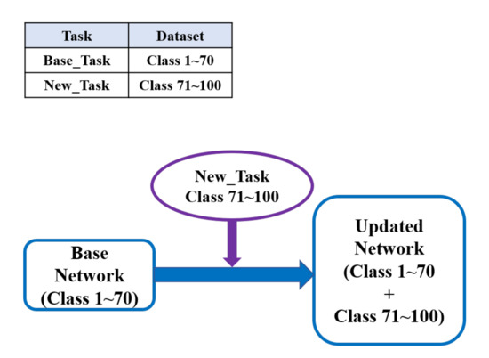
Figure 2.
Incremental learning model: the network needs to accommodate its capacity by updating it with sequential new classes.
4.2. Comparison of Experimental Results for ‘PI’ and ‘EI’
In BayesOpt, the acquisition function is a function that recommends the next candidate to be explored based on the probabilistic estimation of the objective function by the Surrogate Model. We conduct experiments with two types, PI and EI, and compare the results. We utilized the base network which was trained with 70 classes among 100 classes in CIFAR-100 and updated the branch new network with the rest of 30 classes. Then we set the threshold accuracy to 1% less than the baseline accuracy, which did not share any base network layer. Figure 3a shows the result of the selected optimal number of sharing layers through BayesOpt using ‘PI’ as the acquisition function and Figure 4a shows the result of that through BayesOpt using ‘EI’ as the acquisition function. The shaded area represents the uncertainty of unsampled points calculated through GP regression, and the black line is the posterior mean value of unsampled points. The red points denote the normalized loss value of sampled points, and the red line is drawn as the ‘PI’ values based on GP regression results. In Figure 3 and Figure 4b,c, the L2 distance of the consecutive observed points and the value of the calculated best-selected sample are represented for every iteration, respectively. Since ‘PI’ considered only the probability of increasing the function values, while ‘EI’ considers both that and the magnitude of improvements. BayesOpt followed a different path depending on which acquisition function was used as shown in Figure 3 and Figure 4. Therefore, we chose ‘EI’ as an acquisition function that found the better optimal point with the smaller number of attempts.
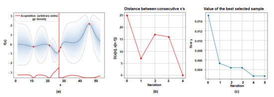
Figure 3.
Visualization results of the optimal sharing layer configuration through BayesOpt using ‘PI’ as the acquisition function. (70 classes/30 classes) (a) the result of the selected optimal number of sharing layers. (b) The L2 distance of the consecutive observed points. (c) The value of the calculated best-selected sample for every iteration.
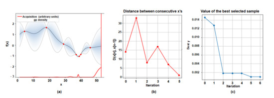
Figure 4.
Visualization results of the optimal sharing layer configuration through BayesOpt using ‘EI’ as the acquisition function. (70 classes/30 classes) (a) The result of the selected optimal number of sharing layers. (b) The L2 distance of the consecutive observed points. (c) The value of the calculated best-selected sample for every iteration.
4.3. Experimental Results on Resnet50 with CIFAR-100
Two cases of the different proportion classes in CIFAR-100 were conducted to demonstrate the proposed algorithm could adaptively find the optimal number of sharing layers considering some threshold accuracy degradation:
- Case 1: utilizing base network which was trained with 70 classes among 100 classes dataset.
- Case 2: utilizing base network which was trained with 60 classes among 100 classes dataset.
4.3.1. Experimental Results on Case 1
We utilized the ‘Case 1’ network and updated the branch new network with the remaining 30 classes. Then we set the threshold accuracy degradation value to 2% less than the baseline accuracy. Figure 5a shows the result of the selected optimal number of sharing layers through BayesOpt. Observing the result, we could find out that the 39th layer was the optimal number of sharing layers with six iterations. This means it could converge to the solution that satisfied the proposed objective function with only six layer-attempts of the experiment. Additionally, since BayesOpt followed the global optimization scheme, the L2 distance of the consecutive points was also very high with updating the best calculated sample value as shown in Figure 5b,c. The combined classification accuracy value of the corresponding sharing layer was 67.84%, while the baseline of classification accuracy was 69.73%, as listed in Table 1. Additionally, we proceeded to experiment with a different threshold value of the combined classification accuracy degradation, such as 3% less than the baseline accuracy, as depicted in Figure 6a–c. Thus, we could get the optimal sharing configuration number of layers to be 47, having an accuracy of 67.03% with only six iterations.
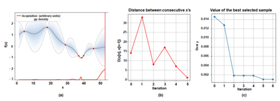
Figure 5.
Visualization results of the optimal sharing layer configuration through BayesOpt as threshold accuracy degradation is 2% less than the baseline accuracy. (70 classes/30 classes) (a) the result of the selected optimal number of sharing layers. (b) The L2 distance of the consecutive observed points. (c) The value of the calculated best-selected sample for every iteration.

Table 1.
Experimental results on the proposed algorithm in CIFAR-100 (Case 1,2).

Figure 6.
Visualization results of the optimal sharing layer configuration through BayesOpt as threshold accuracy degradation is 3% less than the baseline accuracy. (70 classes/30 classes) (a) The result of the selected optimal number of sharing layers. (b) The L2 distance of the consecutive observed points. (c) The value of the calculated best-selected sample for every iteration.
4.3.2. Experimental Results on Case2
We utilized the ‘Case 2’ network which was trained with 60 classes in CIFAR-100 dataset and updated the branch new network with the remaining 40 classes. As shown in Figure 7, the optimal sharing number of layers was 44 in six iterations, when target accuracy degradation was 2% which was lower than the baseline accuracy. As listed in Table 2, The combined classification accuracy of 44 layers sharing in the base network was 67.78% as the baseline accuracy value was 69.81%. Besides, we changed the threshold accuracy value to 3% less than the baseline accuracy, and we could get the result in Figure 8. As listed in Table 1, the optimal sharing layer configuration was 49 in eight iterations, and the combined classification accuracy was 66.82% when the baseline accuracy value was 69.81%.
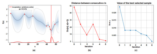
Figure 7.
Visualization results of the optimal sharing layer configuration through BayesOpt BayesOpt as threshold accuracy degradation is 2% less than the baseline accuracy. (60 classes/40 classes) (a) the result of the selected optimal number of sharing layers. (b) The L2 distance of the consecutive observed points. (c) The value of the calculated best-selected sample for every iteration.
Table 2.
Comparison of experimental results for ‘clone and branch’.
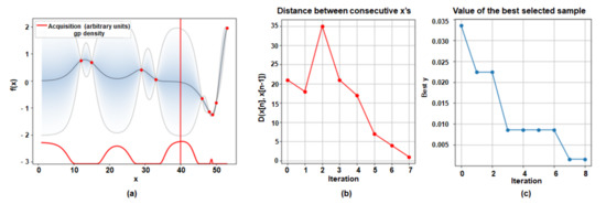
Figure 8.
Visualization results of the optimal sharing layer configuration through BayesOpt BayesOpt as threshold accuracy degradation is 3% less than the baseline accuracy. (60 classes/40 classes) (a) The result of the selected optimal number of sharing layers. (b) The L2 distance of the consecutive observed points. (c) The value of the calculated best-selected sample for every iteration.
4.4. Experimental Results on MobileNetV2 with EMNIST
To evaluate the robustness and the extensive applicability of our proposed methodology, we conducted experiments training another network called MobileNetV2 [34] with EMNIST [35] additionally. EMNIST dataset is set of handwritten character digits derived from the NIST Special Database 19. There are six different splits provided in this dataset, and we used the EMNIST Balanced dataset which contains a set of characters with an equal number of samples per class. It was made up of 131,000 gray characters images, which were converted to 28 × 28 pixel image format and consisted of 47 classes of letters and digits totally. MobileNetV2 is based on an inverted residual structure where the shortcut connections are between the thin bottleneck layer. Besides, the MobileNetV2 network consisted of 52 convolutional layers, and we allowed Bayesian Optimization to select the optimal number of layers within this range. Then, we divided the EMNIST dataset to two sets which were chosen randomly and mutually exclusive. The base network which was trained with 40 classes among 47 classes was utilized and the branch network with the remaining seven classes was updated. To enable the branch network to utilize abundant knowledge acquired from the base network, we trained the base network with most of the 47 classes. The baseline accuracy, where every layer of the network was updated for new tasks without any network sharing, was 78.66% and then we set the threshold accuracy degradation value to 8% less than baseline accuracy. Utilizing the proposed method, the optimal number of sharing layers was obtained as shown in Figure 9. Observing the results of experiment, the optimal number of sharing layers was the 36th layer, having the accuracy of 70.69% with only seven iterations. That means it converged to the optimal solution that satisfies the proposed objective function with only seven layer-attempts of experiment.
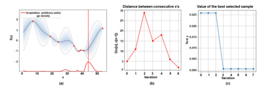
Figure 9.
Visualization results of the optimal sharing layer configuration through BayesOpt BayesOpt as threshold accuracy degradation is 8% less than the baseline accuracy. (EMNIST: 40 classes/seven classes) (a) the result of the selected optimal number of sharing layers. (b) The L2 distance of the consecutive observed points. (c) The value of the calculated best-selected sample for every iteration.
4.5. Comparison of Experimental Results for the ‘Clone and Branch’
In this section, we divided CIFAR-100 into three sets to compare the proposed algorithm with the ‘clone and branch’ technique. The 60 classes (T0) out of the 100 classes were used for training a base network, and the remaining 30 classes (T1) and 10 classes (T2) were used for training each incremental branch network. In Table 2, we set the threshold accuracy of ‘T0–T1’ to 2.33% and that of ‘T0–T2’ to 1.6% for making fair comparisons with ‘clone and branch’ using similarity score [14]. In the case of ‘T0–T1’, the proposed method could achieve the same accuracy result as the ‘clone and branch’ in only four attempts. In case of ‘T0–T2’, we got the same result as the ‘clone and branch’ in nine attempts and since ‘T2’ had 10 classes, which was much smaller than ’Base’, it needed more attempts to converge to reduce the tendency for combined classification accuracy. In other words, despite the same accuracy results of both algorithms, the ‘clone-and-branch’ computationally took a lot of time to obtain the optimal number of sharing layers, searching all cases by increasing the layer one by one for the branch network in the empirical searching step. In Table 2, we could also find out the comparison of computational time between the ‘clone and branch’ technique and the proposed algorithm. We could observe that under the same accuracy results, the computational time required to find the optimal number of sharing layers in our algorithm was reduced by 8.75 times than in the ‘clone and branch’ techniques. (‘clone and branch’ technique: 62.23 h, the proposed algorithm: 7.22 h) Moreover, our proposed algorithm could adaptively find the global optimal sharing configuration with target accuracy via adjusting the threshold accuracy parameters in the proposed loss function.
5. Conclusions
In our work, we introduce a novel methodology for selecting a global optimal sharing layers for incremental learning via BayesOpt. The proposed methodology can adeptly find the number of sharing layers according to a given condition of accuracy degradation by adjusting the threshold accuracy parameter. The experimental results demonstrate that our method finds the precise sharing capacity of a base network for subsequent new tasks and converges in a few iterations. In conclusion, our proposed method is accurate and efficient. We solve the discrete combinatorial optimization problems for incremental learning by BayesOpt, which ensures global convergence.
Author Contributions
Conceptualization, B.K., T.K. and Y.C.; methodology, B.K.; software, B.K.; validation, B.K. and T.K.; formal analysis, T.K.; investigation, B.K.; resources, B.K.; data curation, B.K.; writing—original draft preparation, B.K.; writing—review and editing, B.K.; visualization, B.K.; supervision, T.K. and Y.C.; project administration, Y.C.; funding acquisition, Y.C. All authors have read and agreed to the published version of the manuscript.
Funding
This research received no external funding.
Institutional Review Board Statement
Not applicable.
Informed Consent Statement
Informed consent was obtained from all subjects involved in the study.
Acknowledgments
This work was supported by the National Research Foundation of Korea (NRF) grant funded by the Korea government (Ministry of Science and ICT) (No.1711108458).
Conflicts of Interest
The authors declare no conflict of interest.
Abbreviations
The following abbreviations are used in this manuscript:
| BayesOpt | Bayesian optimization |
| DCNN | Deep convolutional neural network |
Appendix A. Overview of Bayesian Optimization
As in other kinds of optimization, in Bayesian optimization, we are interested in finding the global minimum of an objective function , where x is a sample from the bounded subset of . The major difference between the Bayesian optimization and other optimization techniques is that it composes a probabilistic model of the objective function . After the probabilistic model composition, the Bayesian optimization utilizes this model to make decisions about where in X to next identifies the objective function, while figuring out uncertainty. The basic belief is to use all of the information available from previous evaluations and not commonly rely on local gradient approximations [28,30,36]. Therefore, the Bayesian optimization can find the global optimum of intricate non-convex non-differential functions with comparatively rare evaluations. The employed probabilistic model is usually a Gaussian process [37] because of its desirable statistical and computational characteristics. Additionally, to determine the next point to evaluate, we must define an acquisition function, including probability improvement and expected improvement, which quantifies global optimal point expectation.
References
- Redmon, J.; Divvala, S.; Girshick, R.; Farhadi, A. You Only Look Once: Unified, Real-Time Object Detection. In Proceedings of the IEEE Conference on Computer Vision and Pattern Recognition (CVPR), Las Vegas, NV, USA, 27–30 June 2016; pp. 779–788. [Google Scholar]
- Sun, Y.; Wang, X.; Tang, X. Deep Learning Face Representation from Predicting 10,000 Classes. In Proceedings of the IEEE Conference on Computer Vision and Pattern Recognition, Columbus, OH, USA, 23–28 June 2014; pp. 1891–1898. [Google Scholar]
- French, R.M. Catastrophic forgetting in connectionist networks. Trends Cogn. Sci. 1999, 3, 128–135. [Google Scholar] [CrossRef]
- Martial, M.; Bugaiska, A.; Bonin, P. The stability-plasticity dilemma: Investigating the continuum from catastrophic forgetting to age-limited learning effects. Front. Psychol. 2013, 4, 504. [Google Scholar]
- Biederman, I. Recognition-by-Components: A Theory of Human ImageUnderstanding. Psychol. Rev. 1987, 94, 115–147. [Google Scholar] [CrossRef] [PubMed]
- Bendale, A.; Boult, T. Towards open world recognition. In Proceedings of the Conference on Computer Vision and Pattern Recognition (CVPR), Boston, MA, USA, 7–12 June 2015; pp. 1893–1902. [Google Scholar]
- Goodfellow, I.J.; Mirza, M.; Courville, A.; Bengio, Y. An empirical investigation of catastrophic forgetting in gradient-based neural networks. arXiv 2015, arXiv:1312.6211v3. [Google Scholar]
- Pan, S.J.; Yang, Q. A survey on transfer learning. IEEE Trans. Knowl. Data Eng. 2010, 22, 1345–1359. [Google Scholar] [CrossRef]
- Yosinski, J.; Clune, J.; Bengio, Y.; Lipson, H. How transferable are features in deep neural networks? In Proceedings of the Advances in Neural Information Processing Systems (NIPS), Montreal, QC, Canada, 8–13 December 2014; Volume 27, pp. 1–9. [Google Scholar]
- Zhuang, F.; Qi, Z.; Duan, K.; Xi, D.; Zhu, Y.; Zhu, H.; Xiong, H.; He, Q. A Comprehensive Survey on Transfer Learning. Proc. IEEE 2021, 109, 43–76. [Google Scholar] [CrossRef]
- Li, Z.; Hoiem, D. Learning without Forgetting. IEEE Trans. Pattern Anal. Mach. Intell. 2018, 40, 2935–2947. [Google Scholar] [CrossRef]
- Hinton, G.; Vinyals, O.; Dean, J. Distilling the Knowledge in a Neural Network. arXiv 2015, arXiv:1503.02531. [Google Scholar]
- Michieli, U.; Zanuttigh, P. Knowledge Distillation for Incremental Learning in Semantic Segmentation. arXiv 2019, arXiv:1911.03462. [Google Scholar]
- Sarwar, S.S.; Ankit, A.; Roy, K. Incremental Learning in deep convolutional neural networks using partial network sharing. IEEE Access 2019, 8, 4615–4628. [Google Scholar] [CrossRef]
- Sze, V.; Chen, Y.; Emer, J.; Suleiman, A.; Zhang, Z. Hardware for machine learning: Challenges and opportunities. In Proceedings of the IEEE Custom Integrated Circuits Conference (CICC), Austin, TX, USA, 30 April–3 May 2017; pp. 1–8. [Google Scholar]
- Chen, Y.; Luo, T.; Liu, S.; Zhang, S.; He, L.; Wang, J.; Li, L.; Chen, T.; Xu, Z.; Sun, N.; et al. DaDianNao: A Machine-Learning Supercomputer. In Proceedings of theAnnual IEEE/ACM International Symposium on Microarchitecture, Cambridge, UK, 13–17 December 2014; pp. 609–622. [Google Scholar]
- Maji, P.; Mullins, R. On the Reduction of Computational Complexity of Deep Convolutional Neural Networks. Entropy 2018, 20, 305. [Google Scholar] [CrossRef]
- Simonyan, K.; Vedaldi, A.; Zisserman, A. Deep inside Convolutional Networks: Visualising Image Classification Models and Saliency Maps. In Proceedings of the ICLR, Banff, AB, Canada, 14–16 April 2014; pp. 1–8. [Google Scholar]
- Zeiler, M.D.; Fergus, R. Visualizing and understanding convolutional networks. In Proceedings of the European Conference on Computer Vision, Zurich, Switzerland,6–12 September 2014; Springer: Cham, Switzerland, 2014. [Google Scholar]
- Dumitru, E.; Bengio, Y.; Courville, A.; Vincent, P. Visualizing Higher-Layer Features of a Deep Network; University of Montreal: Montreal, QC, Canada, 2009; Volume 1341, p. 1. [Google Scholar]
- Donahue, J.; Jia, Y.; Vinyals, O.; Hoffman, J.; Zhang, N.; Tzeng, E.; Darrell, T. Decaf: A deep convolutional activation feature for generic visual recognition. In Proceedings of the International Conference on Machine Learning, Beijing, China, 21–26 June 2014. [Google Scholar]
- Haftka, R.T.; Scott, E.P.; Cruz, J.R. Optimization and Experiments: A Survey. Appl. Mech. Rev. 1998, 51, 435–448. [Google Scholar] [CrossRef]
- Hare, W.; Nutini, J.; Tesfamariam, S. A survey of non-gradient optimization methods in structural engineering. Adv. Eng. Softw. 2013, 59, 19–28. [Google Scholar] [CrossRef]
- Krizhevsky, A.; Sulskever, I.; Hinton, G.E. ImageNet classification with deep convolutional neural networks. In Proceedings of the Advances in Neural Information Processing Systems (NIPS), Lake Tahoe, NV, USA, 3–6 December 2012; pp. 1–9. [Google Scholar]
- Kim, T.; Lee, J.; Choe, Y. Bayesian Optimization-Based Global Optimal Rank Selection for Compression of Convolutional Neural Networks. IEEE Access 2020, 8, 17605–17618. [Google Scholar] [CrossRef]
- Kim, T.; Choe, Y. Background subtraction via exact solution of Bayesian L1-norm tensor decomposition. In Proceedings of the International Workshop on Advanced Imaging Technology (IWAIT) 2020, Yogyakarta, Indonesia, 5–7 January 2020; International Society for Optics and Photonics: Washington, DC, USA, 2020; Volume 11515. [Google Scholar]
- Kim, B.; Kim, T.; Choe, Y. A Novel Layer Sharing-based Incremental Learning via Bayesian Optimization. In Proceedings of the MDPI in 1st International Electronic Conference on Applied Sciences session Computing and Artificial Intelligence, Online, 10–30 November 2020. [Google Scholar]
- Frazier, P.I. A tutorial on bayesian optimization. arXiv 2018, arXiv:1807.02811. [Google Scholar]
- Snoek, J.; Larochelle, H.; Adams, R.P. Practical bayesian optimization of machine learning algorithms. In Proceedings of the Advances in Neural Information Processing Systems, Lake Tahoe, NV, USA, 3–6 December 2012. [Google Scholar]
- Brochu, E.; Cora, V.M.; Freitas, N.D. A tutorial on Bayesian optimization of expensive cost functions, with application to active user modeling and hierarchical reinforcement learning. arXiv 2010, arXiv:1012.2599. [Google Scholar]
- Pelikan, M.; Goldberg, D.E.; Cantú-Paz, E. BOA: The Bayesian optimization algorithm. In Proceedings of the Genetic and eVolutionary Computation Conference GECCO-99, Orlando, FL, USA, 13–17 July 1999; Volume 1. [Google Scholar]
- He, K.; Zhang, X.; Ren, S.; Sun, J. Deep residual learning for image recognition. In Proceedings of the IEEE Conference on Computer Vision and Pattern Recognition, Las Vegas, NV, USA, 27–30 June 2016. [Google Scholar]
- Alex, K.; Hinton, G. Learning Multiple Layers of Features from Tiny Images; Technical Report; Citeseer: Princeton, NJ, USA, 2009; Volume 1. [Google Scholar]
- Sandler, M.; Howard, A.; Zhu, M.; Zhmoginov, A.; Chen, L.-C. MobileNetV2: Inverted Residuals and Linear Bottlenecks. In Proceedings of the IEEE Conference on Computer Vision and Pattern Recognition (CVPR), Salt Lake City, UT, USA, 18–23 June 2018. [Google Scholar]
- Cohen, G.; Afshar, S.; Tapson, J.; van Schaik, A. EMNIST: An extension of MNIST to handwritten letters. 2017; arXiv, 1702. [Google Scholar]
- Kushner, H.J. A new method of locating the maximum point of an arbitrary multipeak curve in the presence of noise. J. Basic Eng. 1964, 86, 97–106. [Google Scholar] [CrossRef]
- Rasmussen, C.E.; Williams, C.K.I. Gaussian Processes for Machine Learning (Adaptive Computation and Machine Learning); MIT Press: Cambridge, MA, USA, 2005; ISBN 026218253X. [Google Scholar]


Publisher’s Note: MDPI stays neutral with regard to jurisdictional claims in published maps and institutional affiliations. |
© 2021 by the authors. Licensee MDPI, Basel, Switzerland. This article is an open access article distributed under the terms and conditions of the Creative Commons Attribution (CC BY) license (http://creativecommons.org/licenses/by/4.0/).