Article

Seismic Ground Response Prediction Based on Multilayer Perceptron

Department of Civil and Environmental Engineering, Pusan National University, Busan 46241, Korea
*
Author to whom correspondence should be addressed.
Appl. Sci. 2021, 11(5), 2088; https://doi.org/10.3390/app11052088
Submission received: 28 December 2020 / Revised: 14 February 2021 / Accepted: 16 February 2021 / Published: 26 February 2021
(This article belongs to the Section Civil Engineering)

Abstract

:
Earthquake disasters can cause enormous social and economic damage, and therefore the sustainability of infrastructure requires the mitigation of earthquake consequences. In seismic design of infrastructures, it is essential to estimate the response of the site during earthquake. Geotechnical engineers have developed quantitative methods for analyzing the seismic ground response. This study proposes a multilayer perceptron (MLP) model to evaluate the seismic response of the surface based on the seismic motion at the bedrock (or 100 m level), and compares its performance with that of a conventional model. A total of 6 sites, with 100 earthquake events at each site, were selected from the Kiban Kyoshin Network (KiK-net) and used as datasets. The acceleration response spectra were calculated from the predicted and measured (baseline) acceleration histories and compared. The proposed MLP model predicted the magnitudes of response and the natural periods where the response amplifies closely with the measured ground motions (baseline). The MLP model outperformed the conventional model for seismic ground response analysis. However, the proposed model did not perform as well for earthquakes whose response spectra exceed 2 g due to a deficiency in large earthquake measurements in the training datasets.

1. Introduction

Earthquake disasters can cause enormous social and economic damage [1,2], and therefore the sustainability of infrastructure requires the mitigation of earthquake consequences. Disaster mitigation should consider the seismic performance of structures in response to earthquakes. The bedrock motion may be remarkably amplified on the ground surface [3]. Geotechnical engineers have developed quantitative methods for analyzing the seismic ground response. Seismic ground response analysis refers to the evaluation of acceleration response on the surface based on the characteristics of the soil deposits and the bedrock motions.
Deep learning based on artificial neural networks allows computational models composed of multiple processing layers to learn representations of data with multiple levels of abstraction [4]. Developments in deep learning have opened up new possibilities in the domain of civil engineering [5,6,7]. Cury and Crémona [8] suggested a multilayer perceptron (MLP)-based damage classification scheme for a beam-type structure. Kao and Loh [9] used MLP to present a monitoring method for dam inspection, estimating the long-term deformation of the dam. The MLP model is given the information extracted from the water level and temperature distribution of the dam body. Suresh et al. [10] carried out active control of a base-isolated building with MLP. They approximated the nonlinear control law of the active controller and applied appropriate force from the controller to the building to reduce the vibration response using MLP. Arangio and Beck [11] achieved damage detection, localization, and quantification for bridge structures by incorporating Bayesian inference with MLP. Razavi et al. [12] fit the load-deflection curve of a carbon fiber-reinforced polymer reinforced concrete slab using MLP. Derkevorikian et al. [13] predicted the relative displacement and velocity time history by incorporating MLP and ordinary differential equation (ODE) solver, in which MLP was used to detect damage by modeling the soil-structure interaction. Rih-Teng and Mohammad [14] developed a convolution neural networks (CNN)-based model to estimate the structural dynamic response of a linear single-degree-of-freedom (SDOF) system, a nonlinear SDOF system, and a full-scale 3-story multidegree-of-freedom (MDOF) steel frame.
This study proposes a multilayer perceptron (MLP) model to evaluate the seismic response of the surface based on the seismic motion at the bedrock (or 100 m level) and compares its performance with that of a conventional physical model. The acceleration histories at the surface and bedrock stored in the Japanese database Kiban Kyoshin Network (KiK-net) were used as datasets. A total of 6 sites were selected, and 100 earthquake events at each site were fabricated and used for the MLP model. The spectral accelerations were calculated from the predicted and measured (baseline) acceleration histories and compared. The seismic motion at the surface was evaluated based on the software for conventional seismic response analysis, SHAKE2000 [15], and its results were also compared with the results of the MLP model.

2. Analytical Methods and Dataset

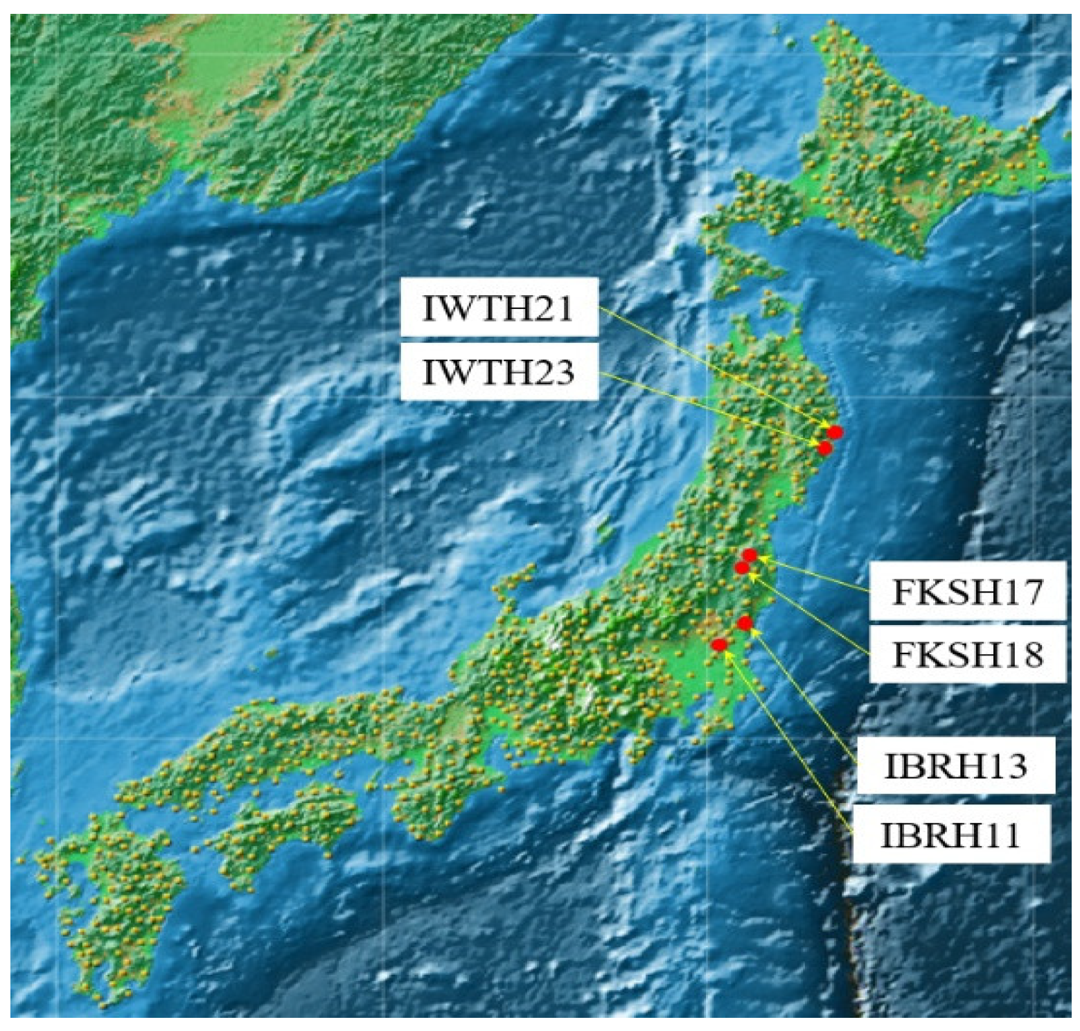
2.1. Earthquake Dataset

Over 90% of earthquakes worldwide occur in the circum-Pacific orogenic zone, known as the Ring of Fire [16]. In Japan, since the Kobe Earthquake in 1995, the National Research Institute for Earth Science and Disaster Prevention (NIED) has implemented seismometers in boreholes and on the ground surface to record earthquakes throughout the nation. The measured acceleration histories and the information of the sites and earthquake events are presented in the strong-motion seismograph network Kiban Kyoshin Network (KiK-net). From KiK-net, a total of six sites where sufficient data about the earthquakes were available were selected (Figure 1). FKSH17 and FKSH18 represent Kawamata and Miharu in Fukushimaken, IBRH11 and IBRH13 represent Iwase and Takahagi in Ibrakiken, and IWTH21 and IWTH23 represent Yamada and Kamaishi in Iwateken.
For modeling, 100 sets of acceleration histories measured at the surface and 100 m depth beneath the surface were selected, with 50 earthquake events measured in two directions, east–west and north–south, providing 100 sets of ground motion accelerations in each site. These 100 sets of acceleration histories can be classified as input data (100 ground motions on the surface) and output data (corresponding 100 ground motions at the bedrock). For input data, the velocity and displacement histories were generated from the acceleration histories at 100 m depth using the software Seismo Signal 2016 [17]. Then, the acceleration, velocity, and displacement histories at 100 m depth were taken as input data in the MLP model. As output data of the model, the acceleration histories at the surface were employed. Out of 100 sets of seismic motion data, 80 datasets from 40 events were used for training (training dataset), and 20 datasets from 10 events for testing (testing dataset).
Figure 2 shows the shear wave velocity (Vs) profiles of the selected sites measured by downhole tests and brief classifications of the soil layers. The black triangles in the figure denote the installation locations of the seismometers.
In the seismic design, the ground stratum can be classified based on the shear wave velocity profile up to 30 m (100 ft) depth beneath the ground [18]. The average shear velocity (Vs,30) is used for the classification and is calculated from Equation (1). The natural period of the soil deposit can theoretically be obtained from Equation (2) when the profile of shear wave velocity is available. The values of average shear velocities and natural periods for six sites are presented in Table 1. The table also includes the depths of the bedrock where the shear wave velocity (Vs) exceeds 1000 and 2000 m/s, respectively.
V s , 30 = 30 i = 1 n H i V s i
T G = 4 i = 1 n H i V s i
where Vs,30 is the shear wave velocity of the strata from the surface up to 30 m below the surface, TG is the natural period ( s ), n is the number of strata from the surface up to 30 m below the surface, Hi is the thickness of stratum i ( m ), and Vsi is the shear wave velocity of stratum i ( m / s ). It is noted that the natural period can also be evaluated from the field measurements. For example, Nakamura [19] showed that the fundamental resonance frequency, which corresponds to the lowest amplification frequency, can be successfully determined by the horizontal-to-vertical spectral-ratio (HVSR) method, especially when a sharp velocity contrast is present at depth.
Based on the National Earthquake Hazard Reduction Program (NEHRP), the sites where Vs,30 ranges from 180 to 360 m/s are classified as stiff soil. The sites where Vs,30 ranges from 360 to 760 m/s are classified as soft rock, and those with Vs,30 over 760 m/s are classified as rock.

2.2. Multilayer Perceptron (MLP) Model

Multilayer perceptron (MLP) is one of the neural network models using the back-propagation training algorithm with the basic form including input, hidden, and output layers [20]. As researchers have recently suggested various architectures to improve MLP performance [21,22,23], it can deal with datasets with high nonlinearity and has been used widely in the civil engineering field.
We modeled the MLP to evaluate the seismic motion at the surface through the bedrock motion (or the motion measured beneath the surface at 100 m depth). Figure 3 presents the schematic of MLP process for the seismic ground response. In the modeling, single hidden layer with 100 neurons was implemented through MLP. Mean squared error (MSE) was applied as the loss function, and the Adam [24] optimizer and rectified linear units (Relu) [25] activation function are employed in the analyses.

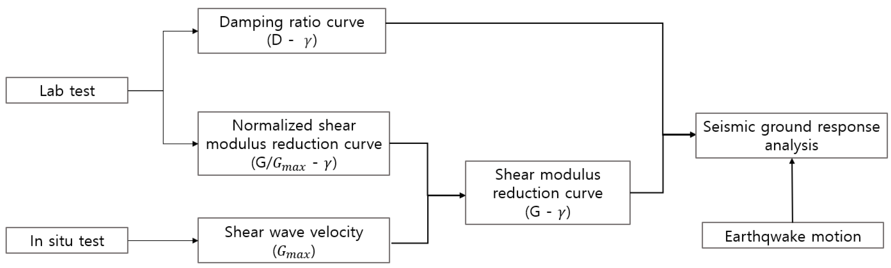
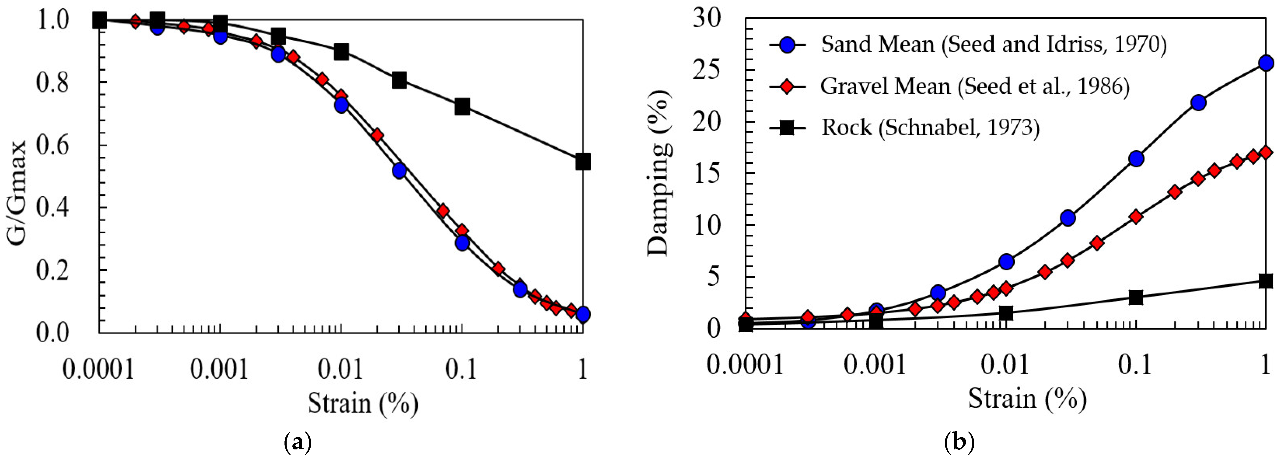
2.3. Conventional Model

Seismic ground response analysis is used to predict the free-field movement on the ground surface during an earthquake [26]. The flow of the seismic ground response analysis is shown in Figure 4. It requires the following input data: the shear moduli of soils at low level of strain, the normalized shear modulus, damping curves as a function of strain, and the earthquake motions at the bedrock or at a certain depth.
We used a computer program SHAKE2000, a conventional physical model for seismic ground response analysis. SHAKE2000 computes the response in a system of homogeneous, viscous-elastic layers of infinite horizontal extent subjected to vertically traveling shear waves. It is based on the continuous solution to the wave-equation adapted for use with transient motions through the Fast Fourier Transform algorithm. The nonlinearity of the shear modulus and damping is taken into consideration for using equivalent linear soil properties with an iterative procedure to obtain values for modulus and damping compatible with the effective strains in each layer [27].
KiK-net provides the profile information of the ground with the types of strata, classified as top soil, sandy gravel, clayey gravel, and granite. The nonlinear dynamic properties of each soil are employed from the proposals in previous literature as shown in Table 2. For the top soil, the mean values of normalized shear modulus and damping ratio curves proposed for sands by Seed and Idriss [28] were taken. For both sandy and clayey gravels, the mean values proposed for gravel by Seed et al. [29] were implemented. The mean values of rocks by Schnabel [30] were used for granite. The shear modulus reduction and damping curves employed are shown in Figure 5.

3. Seismic Responses from MLP and Conventional Models

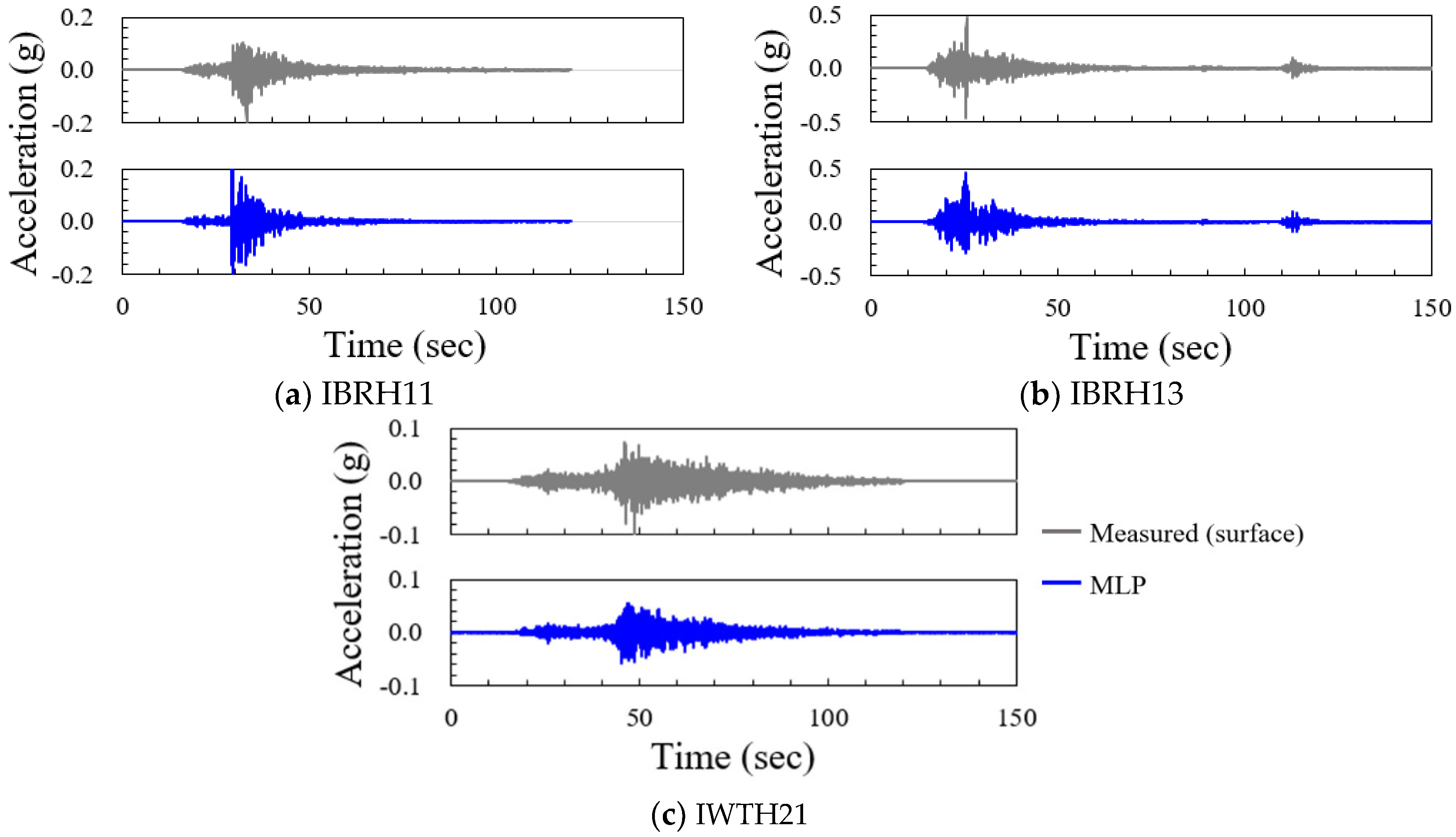
3.1. Acceleration Histories

Examples of the ground motion time histories on the surface measured at stations IBRH11, IBRH13, and IBRH20 and estimated by the MLP model are plotted in Figure 6. The measured and predicted ground motion time histories seem to have similar characteristics.
As a way to conveniently compare the predictions with the measurements and understand the implications of the seismic waves, acceleration response spectra are evaluated from acceleration histories and compared in the following section.

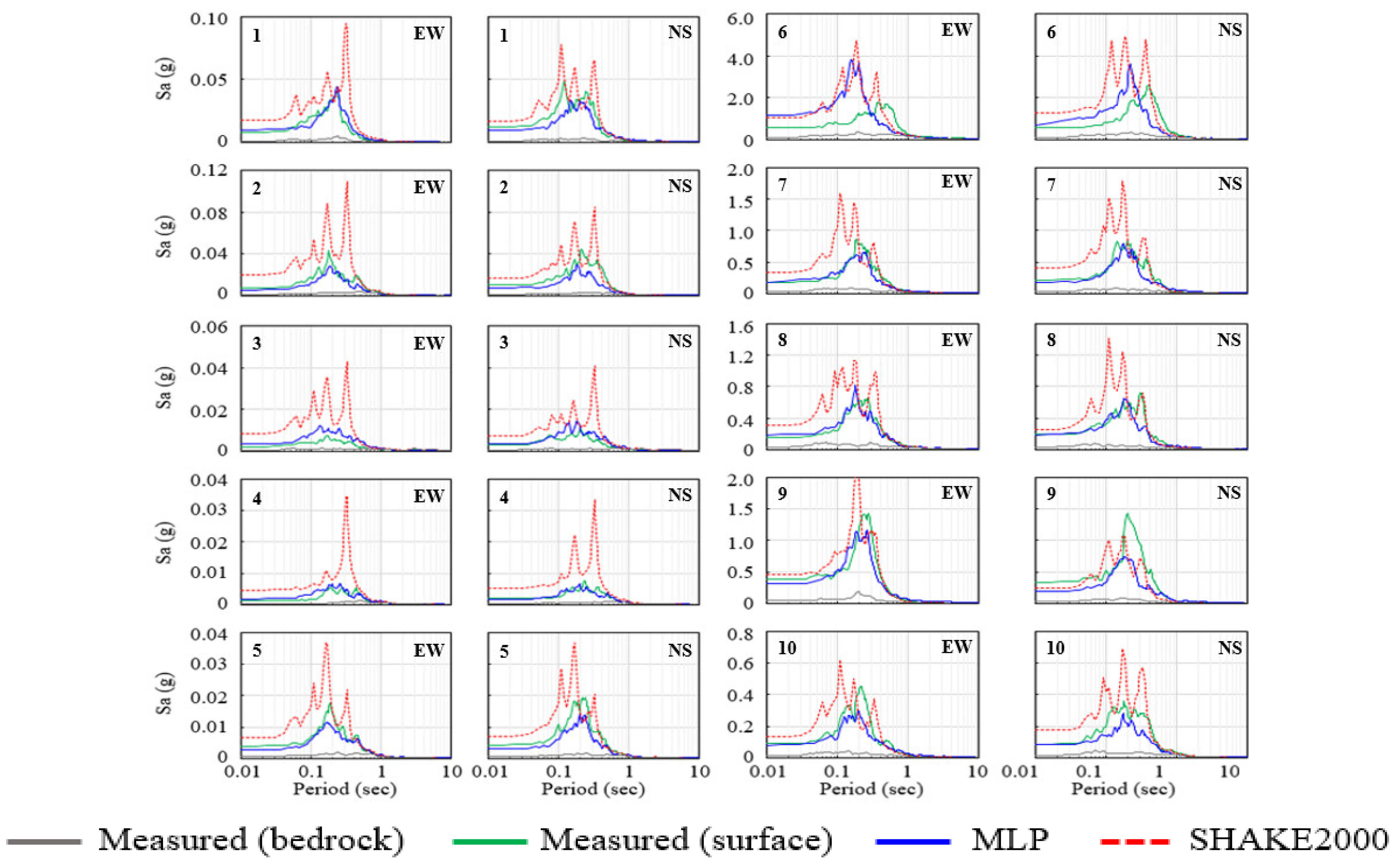
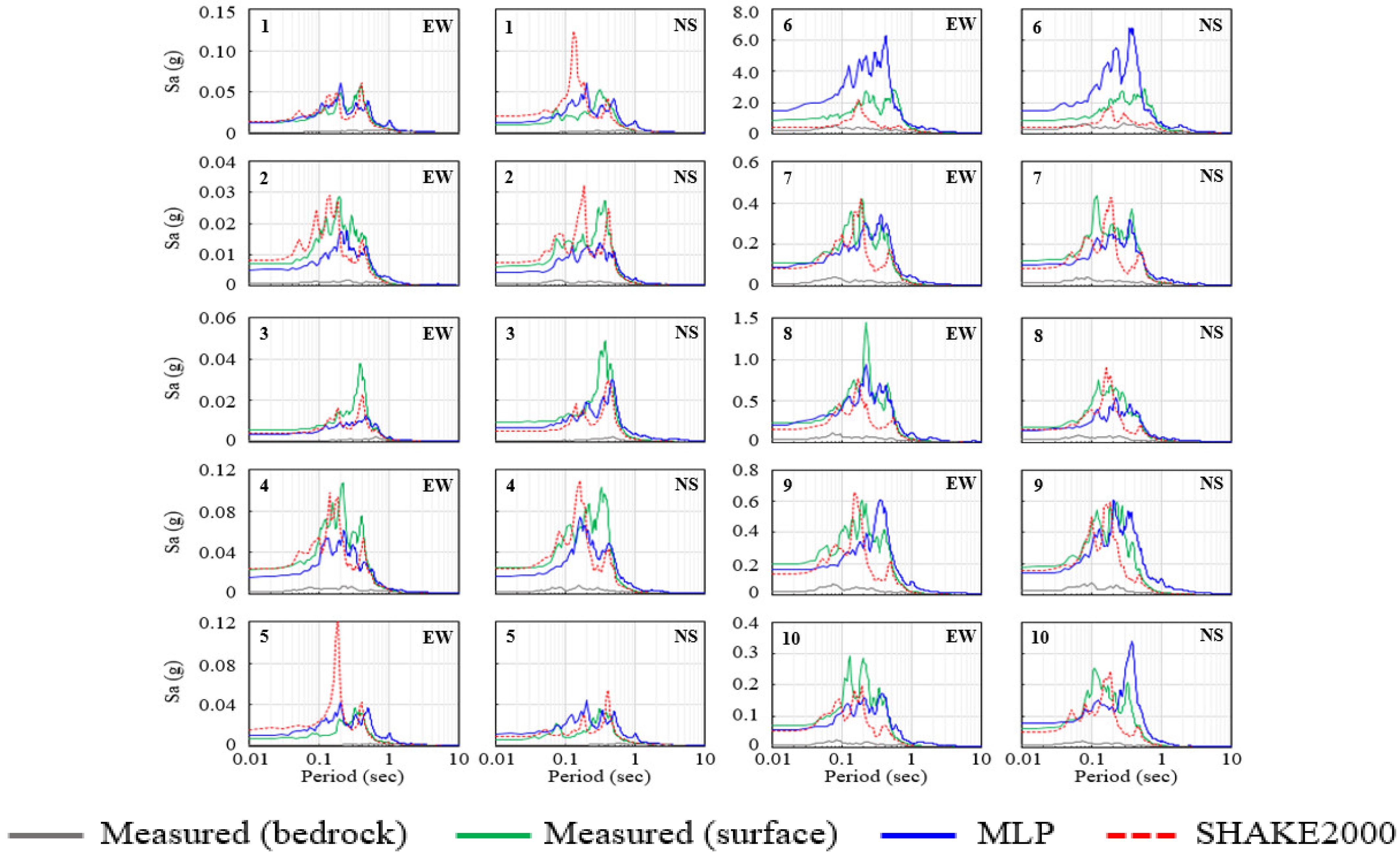
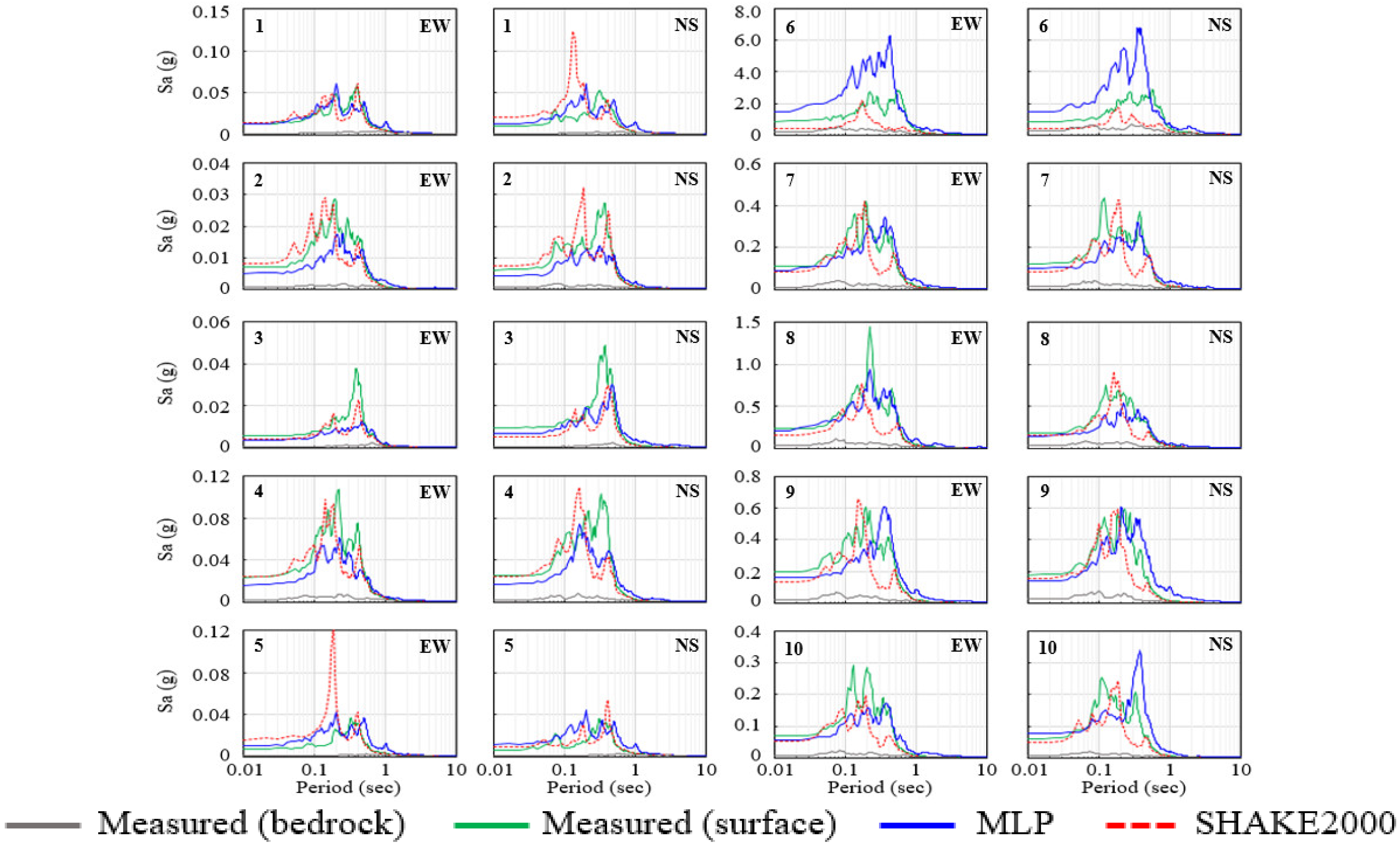
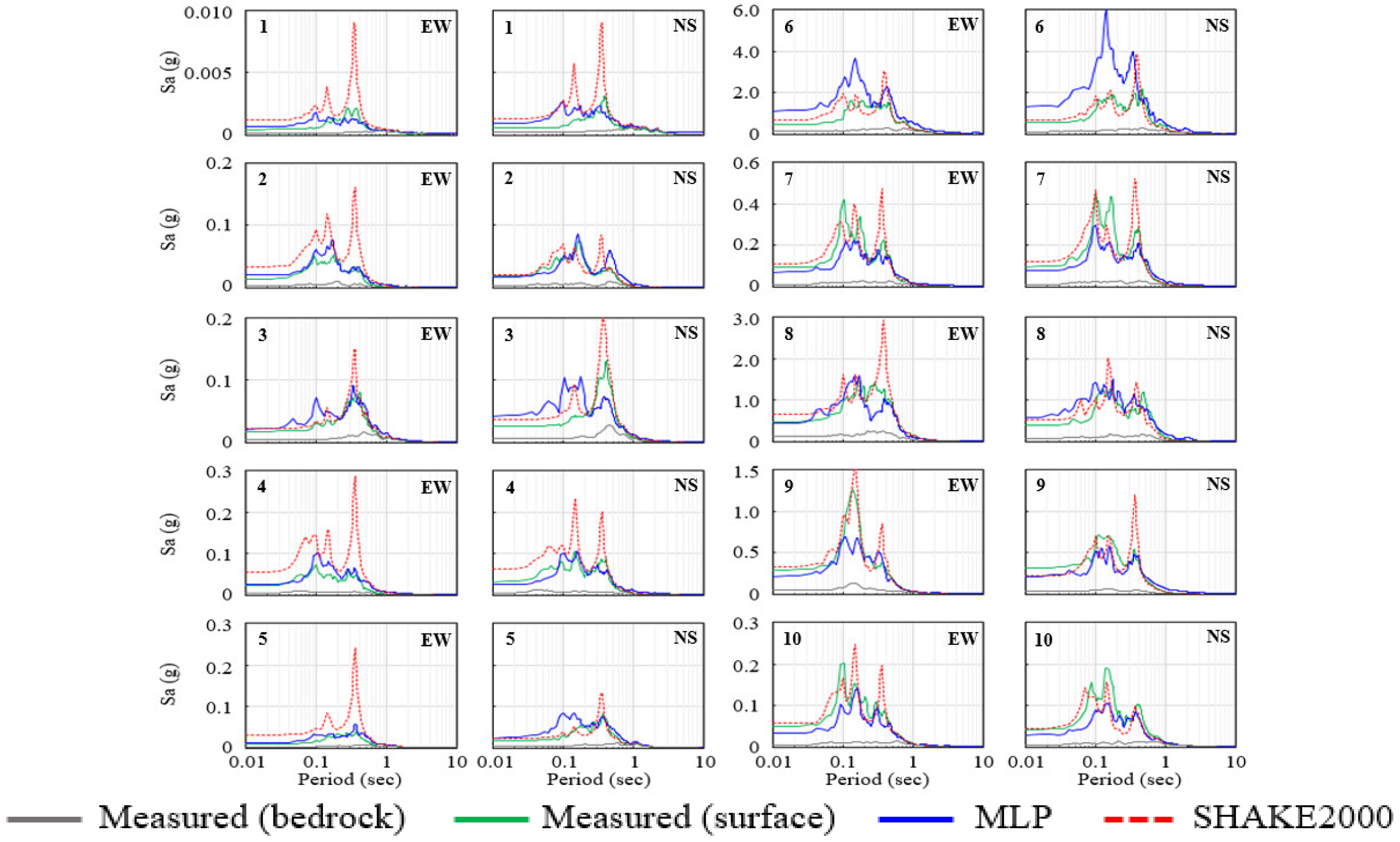
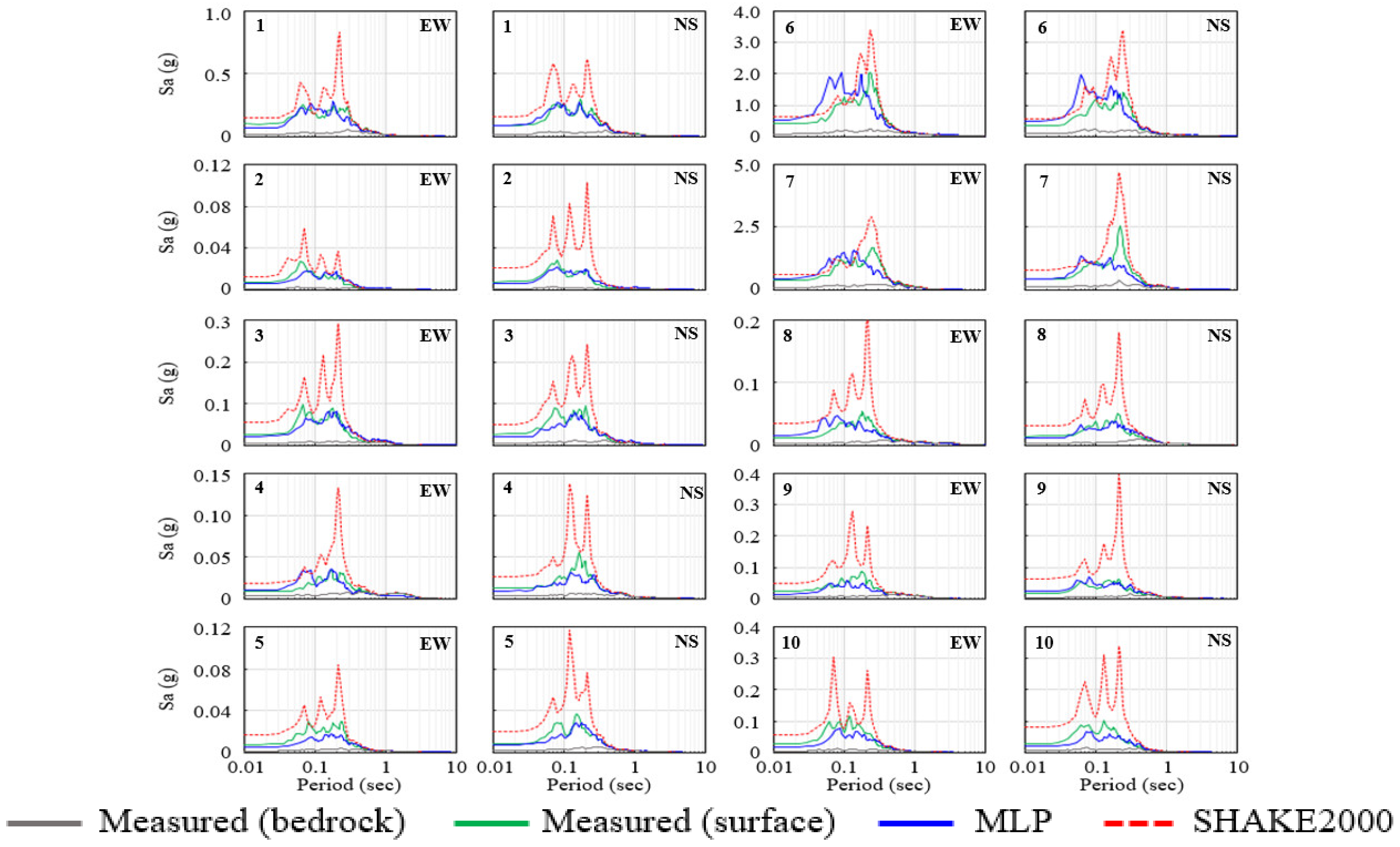
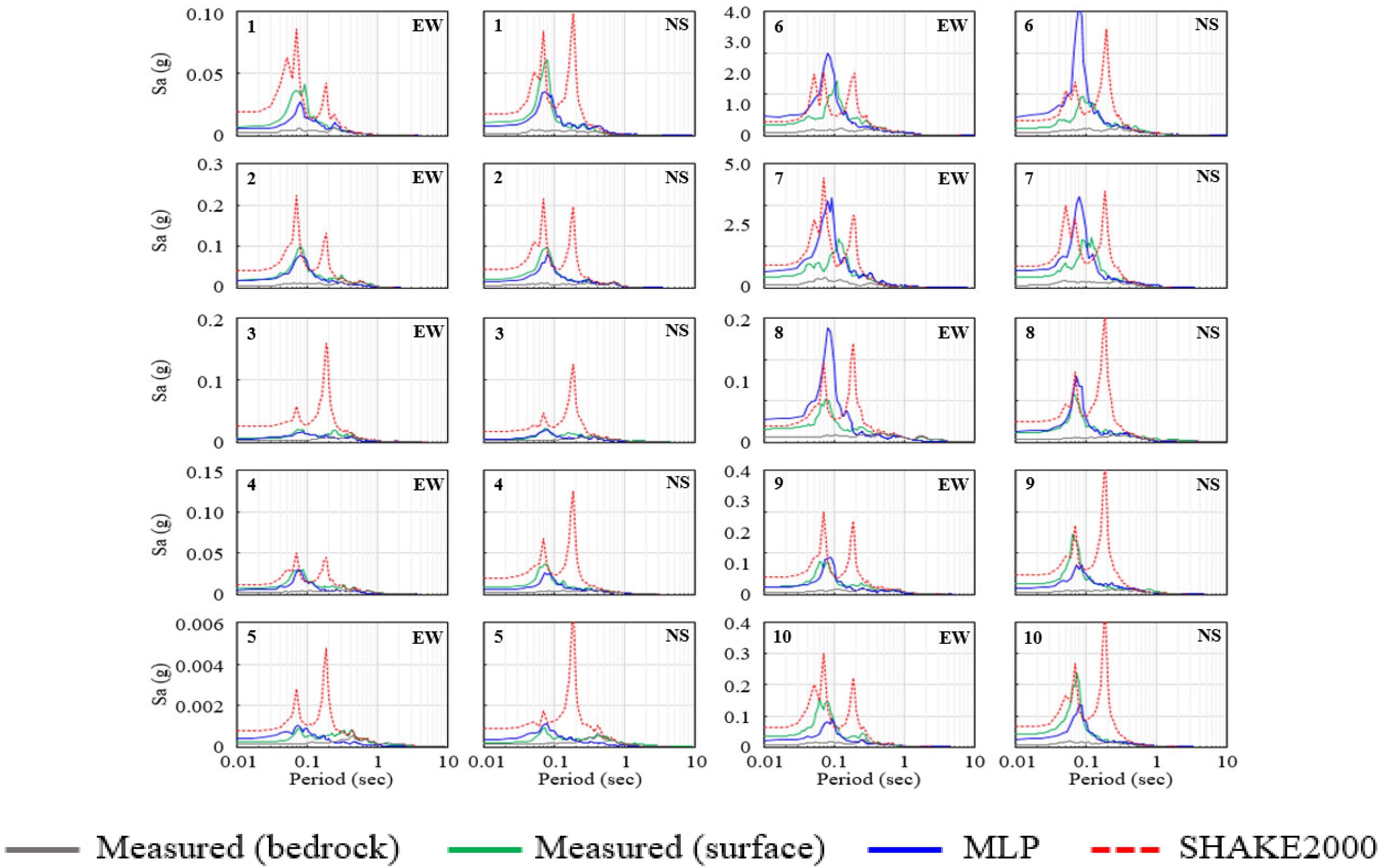
3.2. Response Spectrum

The response spectrum provides a convenient means to summarize the peak response of all possible linear single-degree-of-freedom systems to a particular component of ground motion. It is plotted with the peak value of a response quantity as a function of the natural vibration period of the system. It could be a practical approach to apply knowledge of structural dynamics to the design of structures and development of lateral force requirements in building codes [31].
The acceleration response spectra were generated from the acceleration time histories measured and estimated based on MLP and SHAKE2000. The results of 20 response spectra from 10 earthquake events are plotted and compared in Figure 7, Figure 8, Figure 9, Figure 10, Figure 11 and Figure 12 to investigate the applicability of the MLP model for predicting the ground motion response. In the figures, a number on the left upper side in each graph represents the number of earthquake. EW and NS on the right upper side represent a directions of earthquake events measurement, east–west and north-south.
For the site FKSH17 (Kayamata), the MLP model predicts both the magnitudes of response and the natural periods in which the response amplifies (peaks) very closely with the baseline (measured), with a few exceptions. For example, for the sixth earthquake event whose response spectrum exceeds 2g at most, the MLP model overestimates the response spectrum for the natural periods below 0.3 s. SHAKE2000 tends to overestimate overall the response spectra for all the earthquakes in the site. For the site FKSH18 (Miharu), the MLP model accurately traces the natural periods when the response spectra amplify, although it does not match the magnitudes of response as well as it did in FKSH17. Especially for the sixth earthquake event, it overestimates the motion throughout the natural periods. SHAKE2000 performs as well as the MLP model in this site. In some cases, such as the first and fourth earthquake events, SHAKE2000 predicts even better than the MLP model. It is difficult to say one model is better than the other for this site. For the site IBRH11 (Iwase), both the proposed MLP model and SHAKE2000 match the amplifications of response and the periods where the response amplifies close to the baseline. For the site IBRH13 (Takahagi), while the MLP model shows a similar performance to what it did for IBRH11, SHAKE2000 overestimates the ground response for most earthquakes. For the site IWTH21 (Yamada), the MLP model matches both the magnitudes of response and the natural periods in which the response amplifies closely to the measured response, except for the sixth and seventh earthquakes who have large response spectrum magnitudes. SHAKE2000 especially overestimated the ground response for the most ground responses in the site. For the site IWTH23 (Kamaishi), the MLP model basically matches baselines, with some exceptions—the sixth, seventh, and eighth earthquakes. SHAKE2000 overpredicts for all earthquakes.
Consequently, the MLP model estimates the seismic motions on the surface based on the motions at the bedrock (or 100 m). It, however, tends to overpredict the response when the value of response spectrum at the surface reaches about 2 g. The response spectrum of 2 g is induced by earthquakes with huge magnitude, and earthquakes of this scale are not common in the dataset used for the training of the MLP. As such, the MLP model presented in this study does not present good accuracy for strong earthquakes. When the MLP model is compared with SHAKE2000, the MLP performs better than SHAKE2000 overall. It is, however, noted that the results of SHAKE2000 are dependent on the dynamic properties of the ground employed for the analyses.

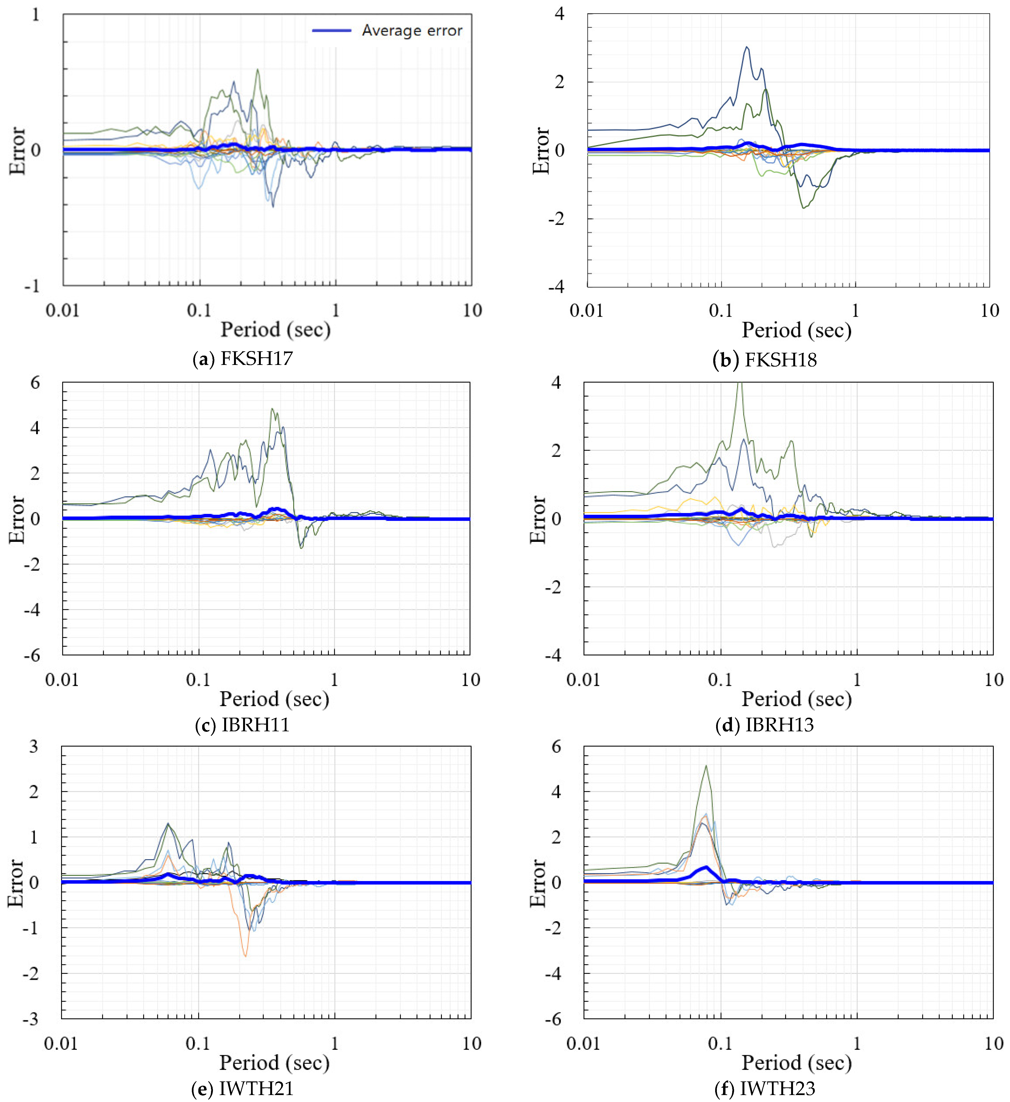
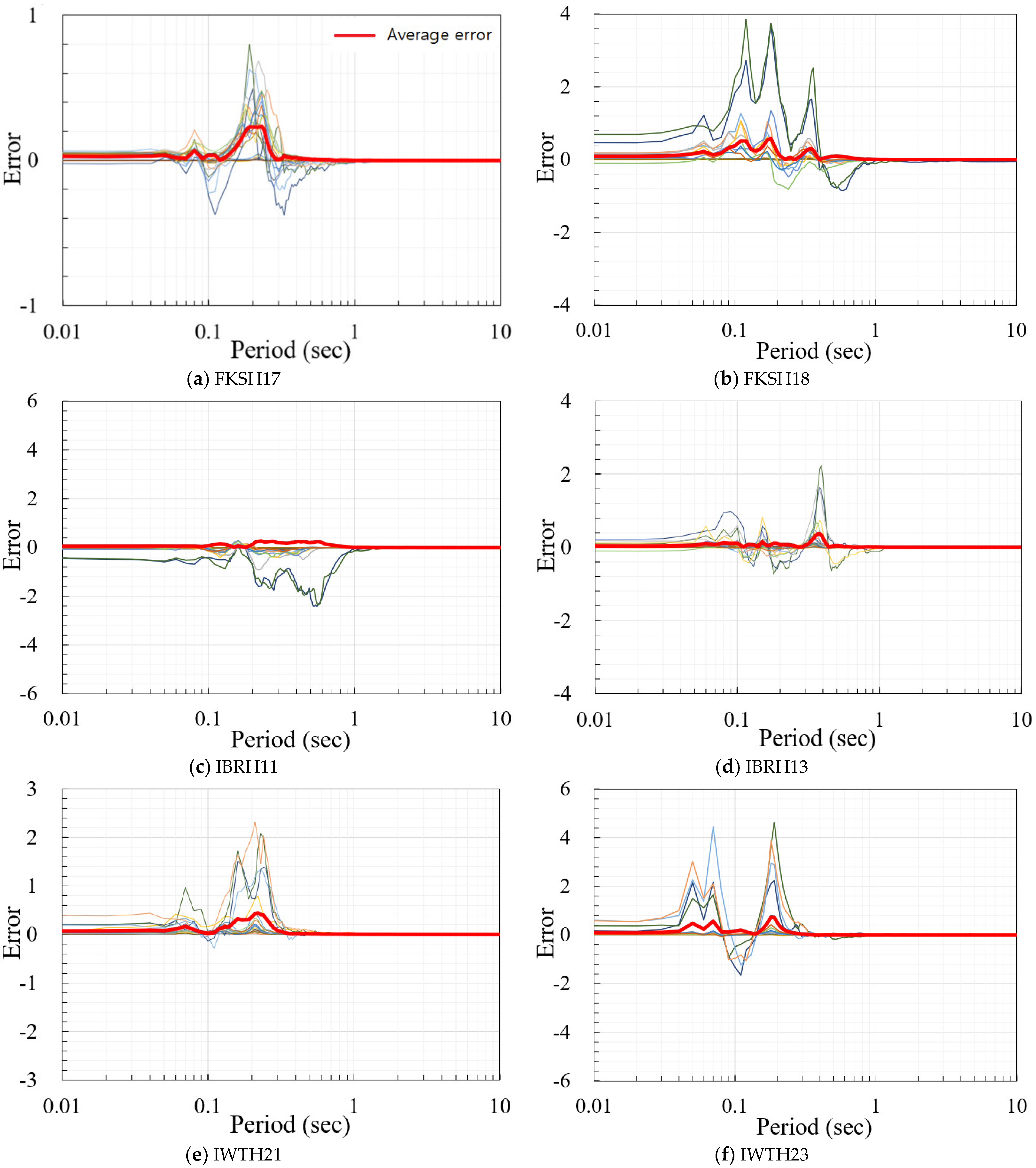
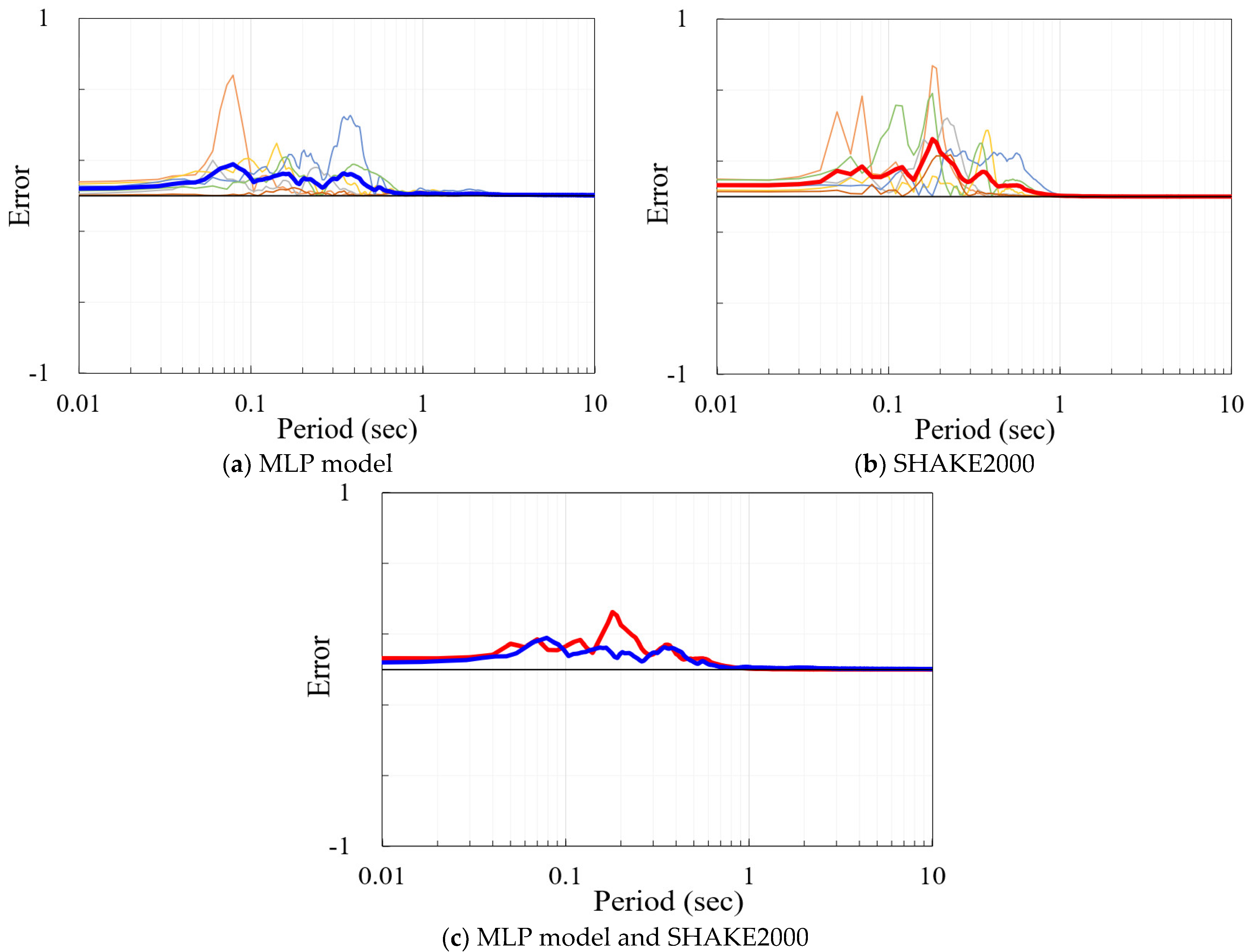
3.3. Prediction Errors

The discrepancy between the response spectra of the models and the baseline of each ground motion was quantified as an error, as presented in Equation (3), for each site.
Error = S a m e a s u r e d S a p r e d i c t e d
where S a m e a s u r e d is the spectral acceleration of the measurement, and S a p r e d i c t e d is the spectral acceleration of the prediction from the MLP or SHAKE2000 model. An average of 20 errors in each station (average error) was calculated with Equation (4):
Average   Error = 1 n i = 1 n ( Error i ) 2
where n is the number of ground motions in each station.
The errors and the average errors of MLP and SHAKE2000 predictions for the six sites are plotted in Figure 13 and Figure 14. In the figures, the thin lines represent errors for 20 individual earthquake measurements, and the thick lines the average of errors for 20 earthquake measurements. For the site FKSH17, the errors are higher for the natural periods between 0.1 and 0.3 s than for other periods. The errors from SHAKE2000 are much higher than those from MLP for this site. For the site FKSH18, both models produced higher errors for the natural periods from 0.1 to 0.5 s. Errors from a large earthquake event caused the most of the average errors (for this site, the sixth earthquake). (for this site, the sixth earthquake). For the sites in Ibarakiken, IBRH11 and IBRH13, both models generated low errors throughout the natural period except for the sixth earthquake. For the site IWTH21, the average errors of the MLP model are low over all the periods as it matches the baseline closely. The average errors of SHAKE2000 seem higher, as it overestimated the response of the ground. For the site IWTH23, the MLP model has larger average errors than SHAKE2000 especially for the periods from 0.06 to 0.1 s. SHAKE2000 outperformed the MLP model in this site.
Even though the results varied a little from site to site, overall, the MLP model produced smaller errors than SHAKE2000. Figure 15 presents and summarizes the total errors of predictions for all sites by MLP and SHAKE2000. The thin lines represent the average errors of the earthquake predictions for each site by Equation (4); the thick lines global errorsof all six sites (all the thin lines) by Equation (5).
Global   Error = 1 n i = 1 n ( Average   Error i ) 2
where n is the number of the sites. The thick blue colored lines are for MLP and the thick red for SHAKE2000.
As shown in Figure 15, the total average errors of the MLP model particularly stand out for the periods from 0.06 to 0.1 s and from 0.3 to 0.5 s. The high average errors for the period between 0.06 and 0.1 s are due to the errors of the site IWTH23, and the errors for the period between 0.3 and 0.5 s are due to those of IBRH11. The average errors of SHAKE2000 are emphasized in the period between 0.1 and 0.3 s by the earthquake measurements from Fukushimaken (FKSH17, FKSH18) and Iwateken (IWTH21, IWTH23).
Throughout the periods, the MLP model outperformed SHAKE2000 in predicting the seismic response on the surface based on the ground motion in the bedrock.

4. Conclusions

This study proposes an MLP-based model to evaluate the seismic response of the surface based on the ground motion at bedrock (or 100 m depth) level, and compares its performance with that of a conventional physical model SHAKE2000. A total of 6 sites in Japan were selected, and 100 ground motions at each site were used for the models. The acceleration response spectra were calculated from the predicted and measured (baseline) acceleration histories for comparison.
The proposed MLP model predicted the magnitudes of response and the natural periods where the response amplifies closely with the measured ground motions (baseline). The proposed model did not perform as well for earthquakes whose response spectra exceed about 2 g due to a deficiency in large earthquake measurements in the training datasets.
The MLP model outperformed the conventional model for seismic ground response analysis, with a few exceptions. It is noted that the seismic ground response analysis by SHAKE2000 was conducted based on the dynamic soil properties widely used in practice. The results of conventional seismic ground response rely greatly on the input properties.
The proposed MLP model incorporates the input and output seismic motions with no soil properties, and therefore it is only applicable for certain sites where the earthquake measurements are available. As a subsequent development, authors aim to implement information of soil layers into the deep learning model so that it can also evaluate the surface ground motion for sites where only the soil information is known.

Author Contributions

Conceptualization and methodology, J.A.; investigation and formal analysis, J.Y., S.H.; validation, J.Y. and J.A.; writing—original draft preparation, J.Y., S.H. and J.A.; review and editing, J.Y., S.H. and J.A. All authors have read and agreed to the published version of the manuscript.

Funding

This research was funded by the Technology Advancement Research Program by the Ministry of Land, Infrastructure, and Transport of the Korean government, grant number 21CTAP-C152100-03.

Data Availability Statement

Data available in a publicly accessible repository that does not issue DOIs. Publicly available datasets were analyzed in this study. This data can be found here: https://www.kyoshin.bosai.go.jp, accessed on 22 February 2021.

Conflicts of Interest

The authors declare no conflict of interest.

References

  1. Green, R.A.; Olson, S.M.; Cox, B.R.; Rix, G.J.; Rathje, E.; Bachhuber, J.; French, J.; Lasley, S.; Martin, N. Geotechnical aspects of failures at Port-auPrince seaport during the 12 January 2010 Haiti earthquake. Earthq. Spectra 2011, 27, 43–65. [Google Scholar] [CrossRef] [Green Version]
  2. Lee, S.H.; Sun, C.G.; Yoon, J.K.; Kim, D.S. Development and verification of a new site classification system and site coefficients for Regions of Shallow Bedrock in Korea. J. Earthq. Eng. 2012, 16, 795–819. [Google Scholar] [CrossRef]
  3. Kramer, S.L. Geotechnical Earthquake Engineering; Prentice Hall: Upper Saddle River, NJ, USA, 2005. [Google Scholar]
  4. LeCun, Y.; Bengio, Y.; Hinton, G. Deep learning. Nature 2015, 521, 436–444. [Google Scholar] [CrossRef] [PubMed]
  5. Adeli, H.; Yeh, C. Preceptron learning in engineering design. Comput.-Aided Civ. Infrastruct. Eng. 1989, 4, 247–256. [Google Scholar] [CrossRef]
  6. Moayedi, H.; Bui, D.T.; Thi Ngo, P.T. Shuffled Frog Leaping Algorithm and Wind-Driven Optimization Technique Modified with Multilayer Perceptron. Appl. Sci. 2020, 10, 689. [Google Scholar] [CrossRef] [Green Version]
  7. Yu, H.; Chen, G.; Gu, H. A machine learning methodology for multivariate pore-pressure prediction. Comput. Geosci. 2020, 143, 104548. [Google Scholar] [CrossRef]
  8. Cury, A.; Crémona, C. Pattern recognition of structural behaviors based on learning algorithms and symbolic data concepts. Struct. Control Health Monit. 2012, 19, 161–186. [Google Scholar] [CrossRef]
  9. Kao, C.-Y.; Loh, C.-H. Monitoring of long-term static deformation data of Fei-Tsui arch dam using artificial neural network-based approaches. Struct. Control Health Monit. 2013, 20, 282–303. [Google Scholar] [CrossRef]
  10. Suresh, S.; Narasimhan, S.; Nagarajaiah, S. Direct adaptive neural controller for the active control of earthquake-excited nonlinear base-isolated buildings. Struct. Control Health Monit. 2012, 19, 370–384. [Google Scholar] [CrossRef]
  11. Arangio, S.; Beck, J.L. Bayesian neural networks for bridge integrity assessment. Struct. Control Health Monit. 2012, 19, 3–21. [Google Scholar] [CrossRef]
  12. Razavi, S.V.; Jumaat, M.Z.; Ahmed, H.E.-S.; Ronagh, H.R. Load-deflection analysis of CFRP strengthened RC slab using focused feed-forward time delay neural network. Concr. Res. Lett. 2014, 5, 858–872. [Google Scholar]
  13. Derkevorkian, A.; Hernandez-Garcia, M.; Yun, H.-B.; Masri, S.F.; Li, P. Nonlinear data-driven computational models for response prediction and change detection. Struct. Control Health Monit. 2015, 22, 273–288. [Google Scholar] [CrossRef]
  14. Wu, R.-T.; Jahanshahi, M.R. Deep convolutional neural network for structural dynamic response estimation and system identification. J. Eng. Mech. 2019, 145, 04018125. [Google Scholar] [CrossRef]
  15. Schnabel, P.B.; Lysmer, J.; Seed, H.B. SHAKE: A Computer Program for Earthquake Response Analysis of Horizontally Layered Sites; Report No. UCB/EERC-72/12; University of California: Berkeley, CA, USA, 1972. [Google Scholar]
  16. Smalley, R., Jr.; Ellis, M.A.; Paul, J.; Van Arsdale, R.B. Space geodetic evidence for rapid strain rates in the New Madrid seismic zone of central USA. Nature 2005, 435, 1088–1090. [Google Scholar] [CrossRef] [PubMed]
  17. Seismosoft Home Page. Available online: https://seismosoft.com/products/seismosignal (accessed on 12 March 2020).
  18. Building Seismic Safety Council (US); Federal Emergency Management Agency. NEHRP Recommended Provisions for the Development of Seismic Regulations for New Buildings; BSSC: Washington, DC, USA, 1988. [Google Scholar]
  19. Nakamura, Y.A. Method for Dynamic Characteristics Estimation of Subsurface Using Microtremor on the Ground Surface; Railway Technical Research Institute, Quarterly Reports: Tokyo, Japan, January 1989. [Google Scholar]
  20. Belue, L.M.; Bauer, K.W. Determining input features for multilayer perceptrons. Neurocomputing 1995, 7, 111–121. [Google Scholar] [CrossRef]
  21. Giles, C.L.; Maxwell, T. Learning, invariance, and generalization in high-order neural networks. Appl. Opt. 1987, 26, 4972–4978. [Google Scholar] [CrossRef] [PubMed]
  22. Chiang, C.-C.; Fu, H.-C. A variant of second order multilayer perceptron and its application to function approximations. In Proceedings of the International Joint Conference on Neural Networks, Baltimore, MD, USA, 7–11 June 1992; pp. 887–892. [Google Scholar] [CrossRef]
  23. Piazza, F.; Uncini, A.; Zenobi, M. Artificial neural networks with adaptive polynomial activation function. In Proceedings of the International Joint Conference on Neural Networks, Beijing, Hebei, China, 7–11 June 1992; pp. 343–348. [Google Scholar]
  24. Kingma, D.P.; Ba, J. Adam: A method for stochastic optimization. arXiv 1412, arXiv:1412.6980. [Google Scholar]
  25. Nair, V.; Hinton, G.E. Rectified linear units improve restricted boltzmann machines. In Proceedings of the 27th International Conference on Machine Learning, Haifa, Israel, 21–24 June 2010. [Google Scholar]
  26. Yoshida, N. Seismic Ground Response Analysis; Springer: Dordrecht, The Netherlands, 2015. [Google Scholar]
  27. GeoMotions, LCC Home Page. Available online: http://geomotions.com (accessed on 20 December 2020).
  28. Seed, H.B.; Idriss, I.M. Soil Moduli and Damping Factors for Dynamic Response Analysis; Report No. EERC 70-10; University of California: Berkeley, CA, USA, 1970. [Google Scholar]
  29. Seed, H.B.; Wong, R.T.; Idriss, I.M.; Tokimatsu, K. Moduli and damping factors for dynamic analysis of cohesionless soils. J. Geotech. Eng. 1986, 112, 1016–1032. [Google Scholar] [CrossRef]
  30. Schnabel, P.B. Effects of Local Geology and Distance from Source on Earthquake Ground Motions; University of California: Berkeley, CA, USA, 1973. [Google Scholar]
  31. Chopra, A.K. Dynamics of Structures: Theory and Applications to Earthquake Engineering; Prentice Hall: Upper Saddle River, NJ, USA, 2017. [Google Scholar]
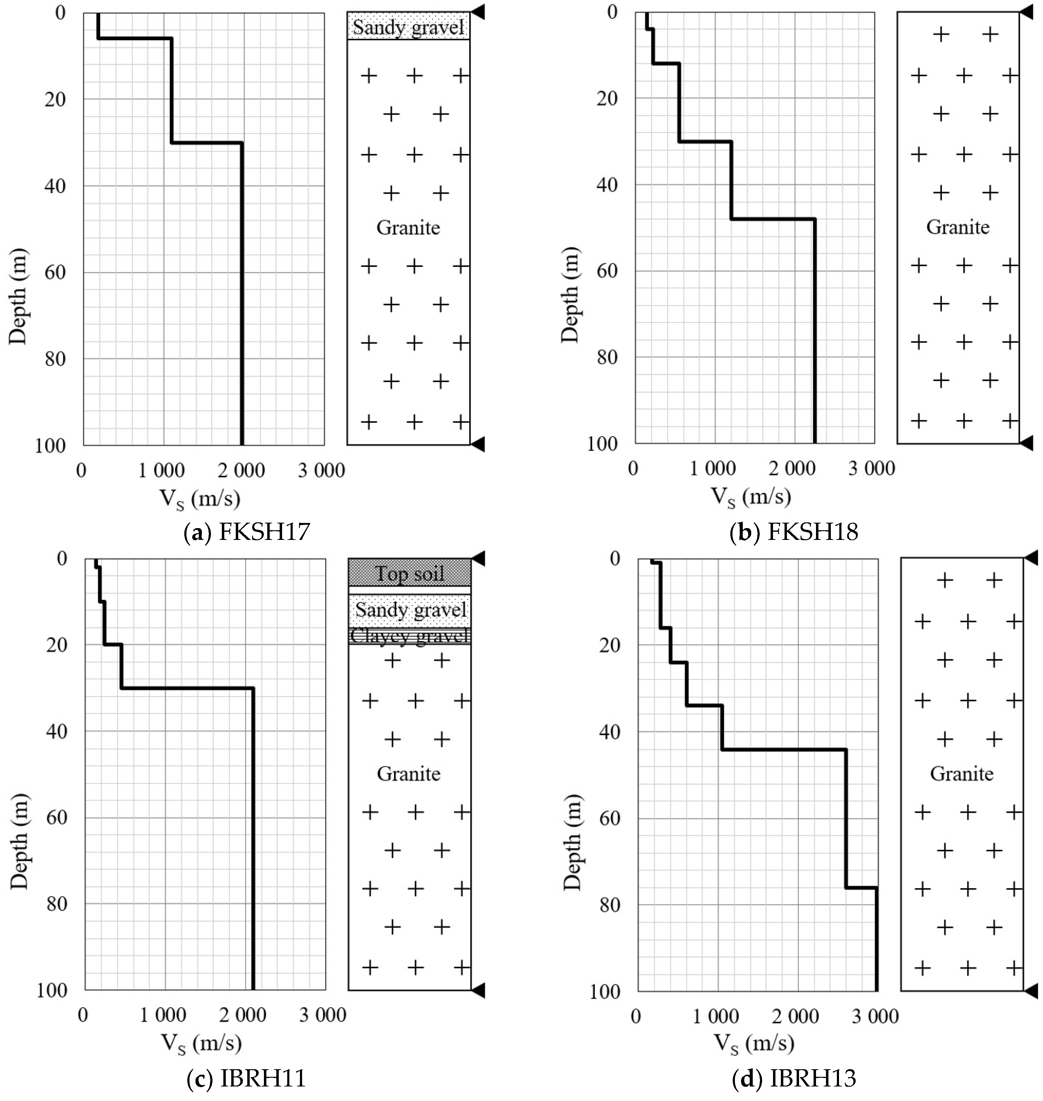
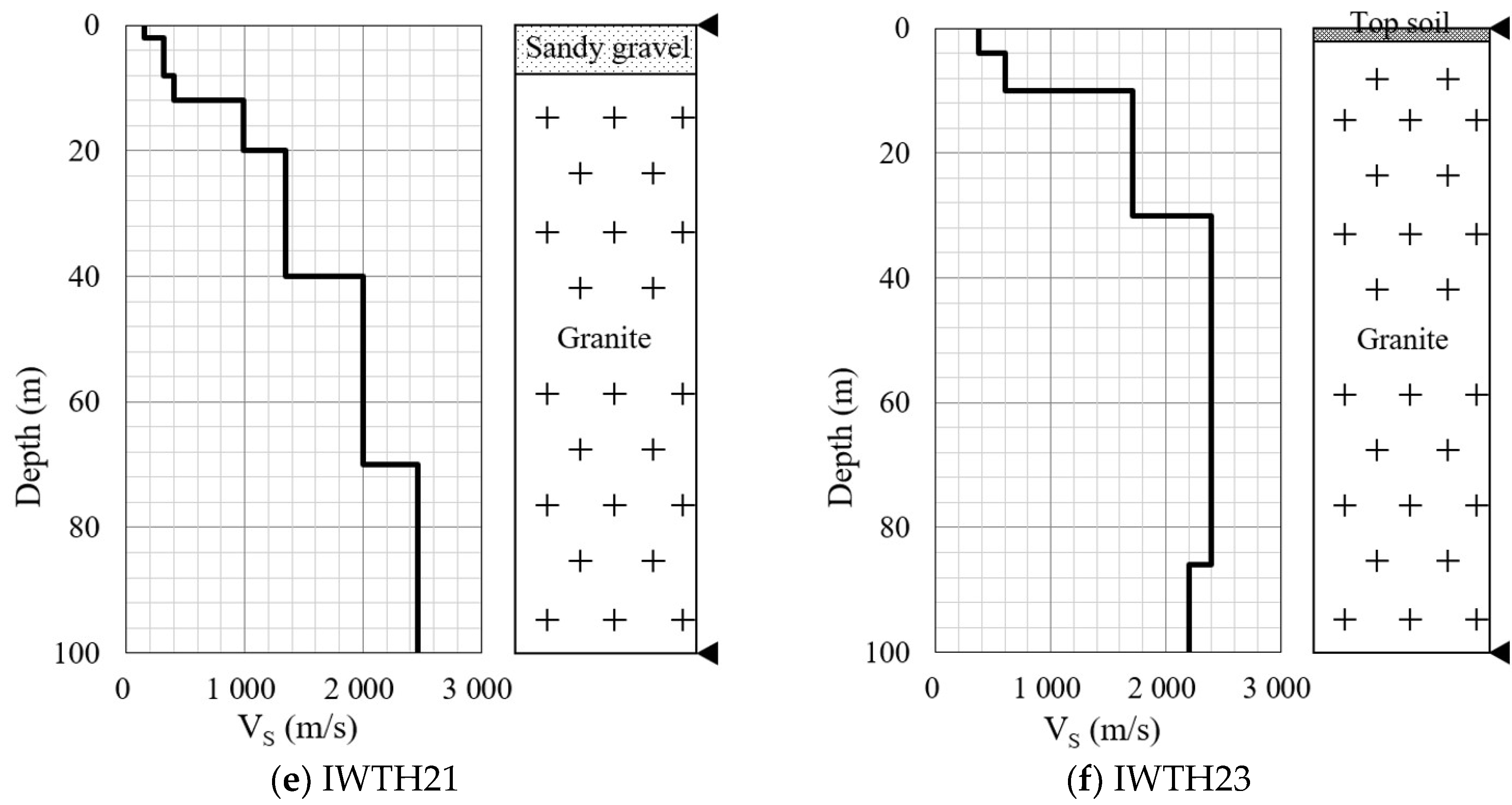
Figure 1. Six stations selected.
Applsci 11 02088 g001
Figure 2. Soil profiles and shear wave velocities at the sites.
Applsci 11 02088 g002aApplsci 11 02088 g002b
Figure 3. Schematic of MLP process for the seismic ground response analysis.
Applsci 11 02088 g003
Figure 4. Flow of seismic ground response analysis.
Applsci 11 02088 g004
Figure 5. Dynamic soil properties: (a) normalized shear modulus reduction curves; (b) damping ratio curves.
Applsci 11 02088 g005
Figure 6. Earthquake acceleration measurements and acceleration predictions by MLP.
Applsci 11 02088 g006
Figure 7. Measured, predicted, and computed response spectra at FKSH17 for east–west and north–south directions.
Applsci 11 02088 g007
Figure 8. Measured, predicted, and computed response spectra at FKSH18 for east–west and north–south directions.
Applsci 11 02088 g008
Figure 9. Measured, predicted, and computed response spectra at IBRH11 for east–west and north–south directions.
Applsci 11 02088 g009
Figure 10. Measured, predicted, and computed response spectra at IBRH13 for east–west and north–south directions.
Applsci 11 02088 g010
Figure 11. Measured, predicted, and computed response spectra at IWTH21 for east–west and north–south directions.
Applsci 11 02088 g011
Figure 12. Measured, predicted, and computed response spectra at IWTH23 for east–west and north–south directions.
Applsci 11 02088 g012
Figure 13. Errors in the ground motions by the MLP model.
Applsci 11 02088 g013
Figure 14. Errors in the ground motions by SHAKE2000.
Applsci 11 02088 g014
Figure 15. The global errors in the earthquake predictions for all sites.
Applsci 11 02088 g015
Table 1. Average shear wave velocity and natural period for each station.
Station V s , 30
( m / s )
T G
( s )
Depth
where Vs is over 1000 m/s
(m)
Depth
where Vs is over 2000 m/s
(m)
FKSH17544.00.22630
FKSH18307.20.393048
IBRH11242.50.493030
IBRH13335.40.363444
IWTH21521.10.232040
IWTH23922.90.131030
Table 2. Description, normalized shear modulus and damping ratio curves.
DescriptionAssumed Type of SoilNormalized Shear Modulus and Damping Ratio Curves
Top soilSand (Mean)Seed and Idriss, 1970
Sandy & Clayey GravelGravel (Mean)Seed et al., 1986
GraniteRock (Mean)Schnabel, 1973
Publisher’s Note: MDPI stays neutral with regard to jurisdictional claims in published maps and institutional affiliations.

