
Outlier Detection for Multivariate Time Series Using Dynamic Bayesian Networks


Abstract
1. Introduction
2. Theoretical Background
2.1. Bayesian Networks
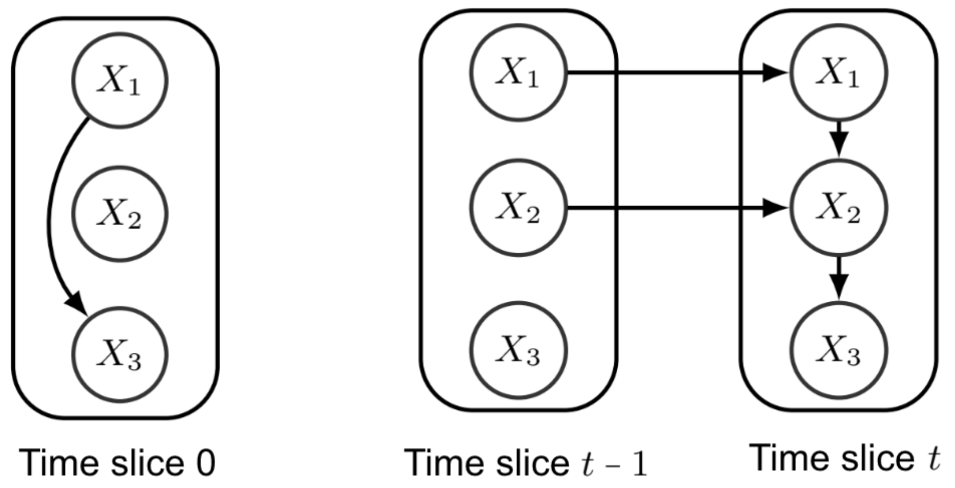
2.2. Dynamic Bayesian Networks
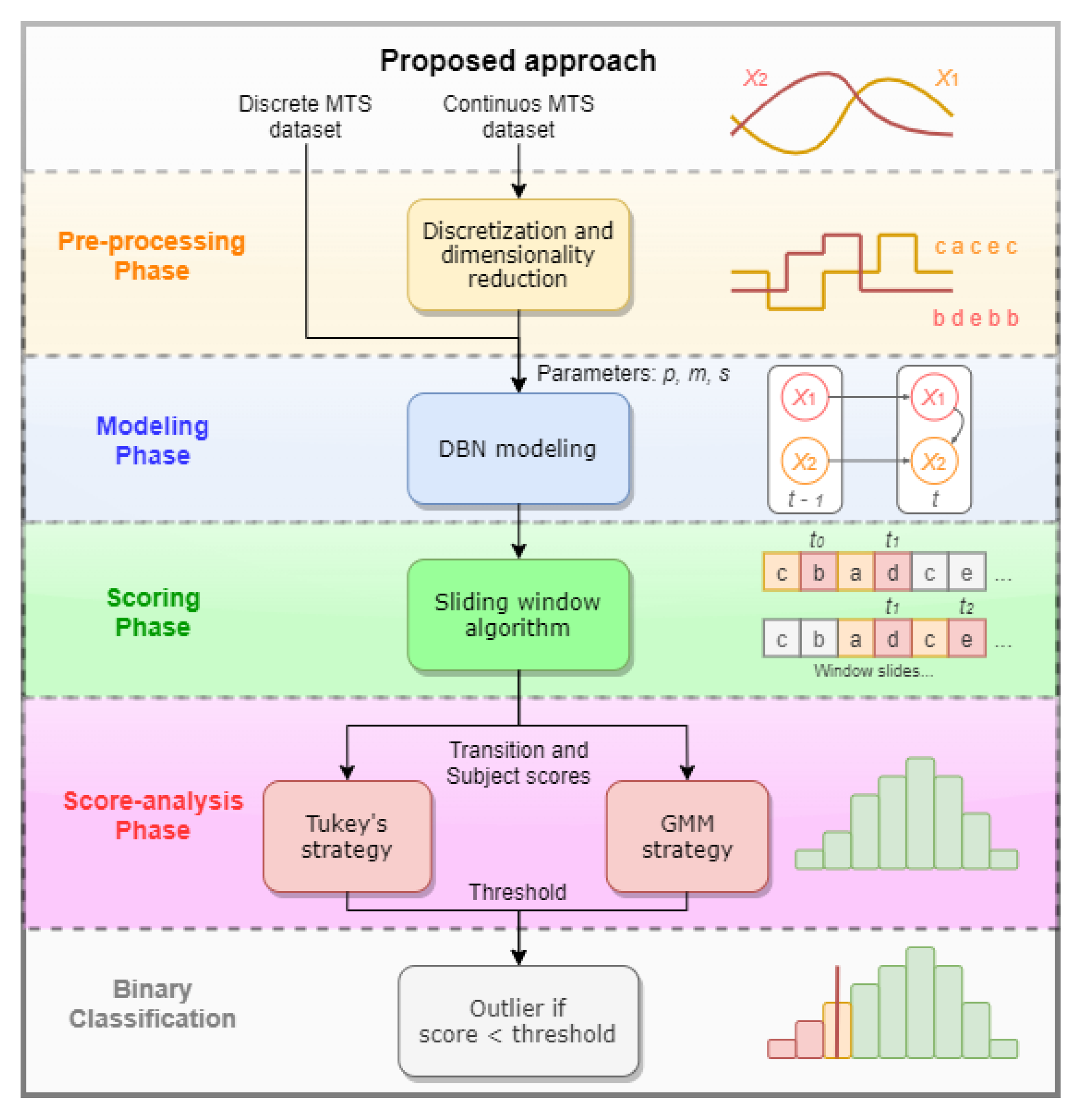
3. Methods
3.1. Pre-Processing
| Algorithm 1 Data Pre-Processing |
|
Input: A MTS dataset D of n variables along T instants; an alphabet size for each attribute , ; desired length of the resulting MTS. Output: The set of input MTS discretized. 1: procedure SAX(D, for all i,w) 2: for each subject h in D do 3: for each TS , with do 4: for each t, with do 5: Normhihi[t] ▹Normalization 6: function PAA() ▹Dimensionality reduction 7: 8: Partition the in contiguous blocks of size 9: for each block do 10: ▹ Compressed slices 11: 12: function Discretization () ▹ Symbolic discretization 13: ) 14: for each value in do 15: Discretehi[k] 16: ▹ Return discretized MTS dataset |
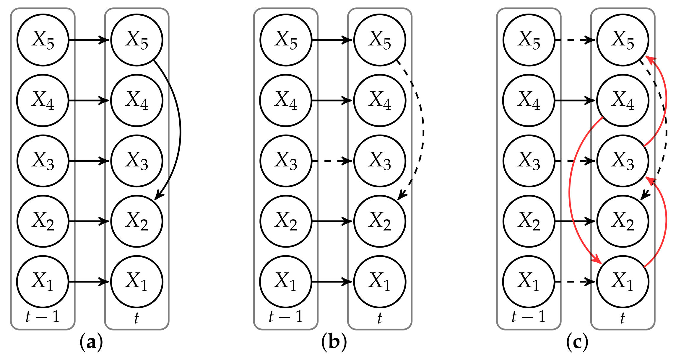
3.2. Modeling
| Algorithm 2 Optimal Non-Stationary m-Order Markov tDBN Learning |
|
Input: A set of input MTS discretized over w time slices; the Markov lag m; the maximum number of parents p from preceding time slices. Output: A tree-augmented DBN structure. 1: procedure Tree-augmented DBN(MTS,m,p) 2: for each transition do 3: Build a complete directed graph in 4: Calculate the weight of all edges and the optimal set of parents 5: Apply a maximum branching algorithm 6: Extract transition network and the optimal set of parents 7: Collect transition networks to obtain a tDBN structure |
3.3. Scoring
| Algorithm 3 Transition Outlier Detection |
|
Input: A tDBN storing conditional probabilities for each transition network , a (discretized) MTS dataset D, and a threshold to discern abnormality. Output: The set of anomalous transitions with scores below . 1: procedure 2: for each time slice t do 3: for each subject do 4: function Scoring() 5: for each variable do 6: ΠXi[t] 7: whi[t] 8: phi 9: Phi ▹ Probability smoothing 10: sht−m:t ▹ Transition score 11: if then 12: outliers .append |
3.4. Parameter Tuning
3.5. Score-Analysis
3.5.1. Tukey’s Strategy
3.5.2. Gaussian Mixture Model
4. Experimental Results
4.1. Simulated Data
4.1.1. Tukey’s Score-Analysis
4.1.2. Gaussian Mixture Model
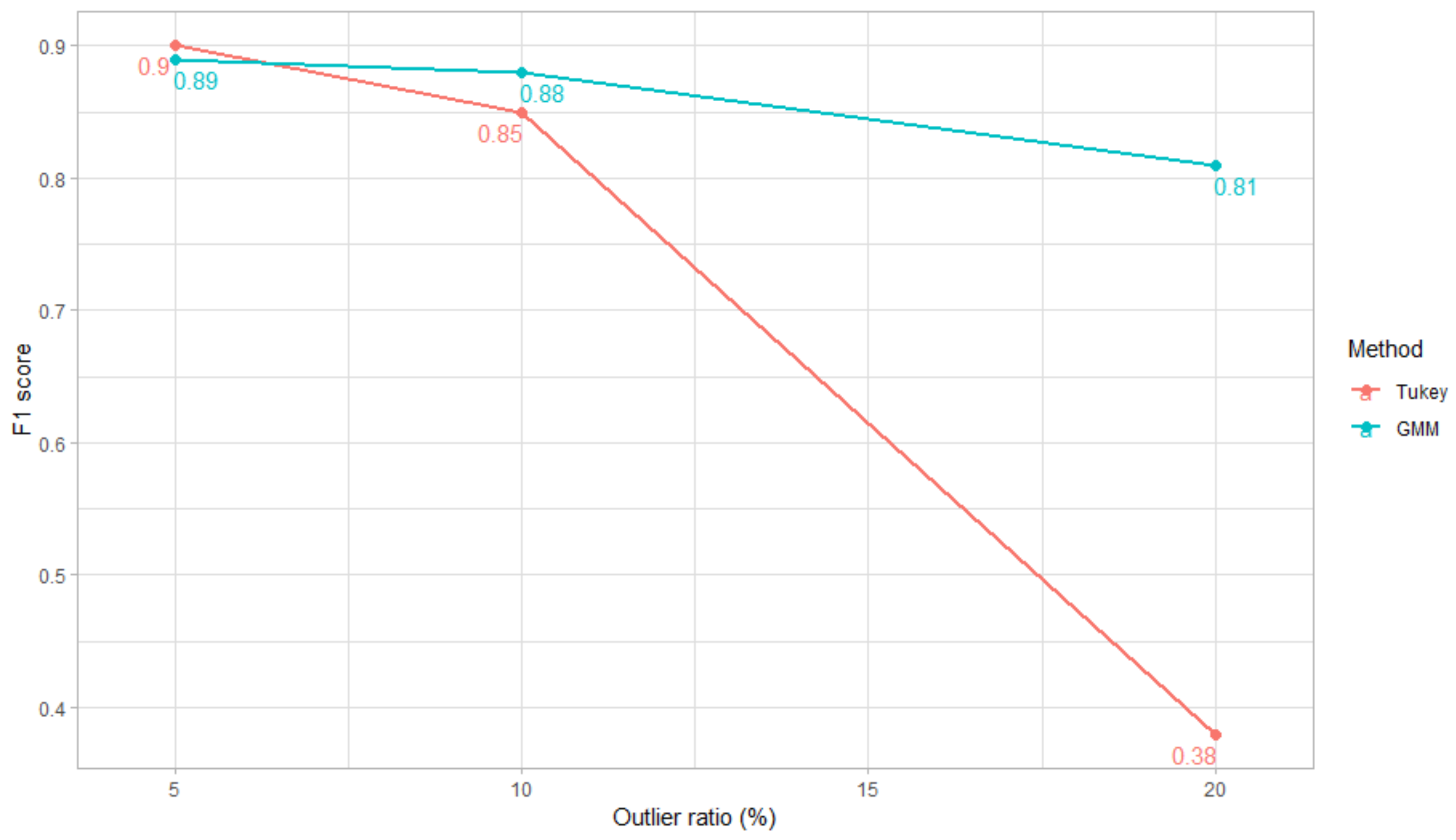
4.1.3. Comparison between GMM and Tukey’s Score-Analysis
4.1.4. Comparison with Probabilistic Suffix Trees
4.2. ECG
4.3. Mortality
4.4. Pen-Digits
5. Conclusions
Author Contributions
Funding
Data Availability Statement
Conflicts of Interest
References
- Grubbs, F.E. Procedures for detecting outlying observations in samples. Technometrics 1969, 11, 1–21. [Google Scholar] [CrossRef]
- López-de Lacalle, J. tsoutliers: Detection of Outliers in Time Series; R Package Version 0.6-6; The Comprehensive R Archive Network (CRAN): Wien, Austria, 2017. [Google Scholar]
- Matt Dancho, D.V. anomalize: Tidy Anomaly Detection; R Package Version 0.1.1; The Comprehensive R Archive Network (CRAN): Wien, Austria, 2018. [Google Scholar]
- Chandola, V.; Banerjee, A.; Kumar, V. Anomaly detection: A survey. ACM Comput. Surv. (CSUR) 2009, 41, 15. [Google Scholar] [CrossRef]
- Aggarwal, C.C. Outlier Analysis; Springer: Berlin, Germany, 2017. [Google Scholar]
- Gupta, M.; Gao, J.; Aggarwal, C.C.; Han, J. Outlier Detection for Temporal Data: A Survey. IEEE Trans. Knowl. Data Eng. 2014, 26, 2250–2267. [Google Scholar] [CrossRef]
- Galeano, P.; Peña, D.; Tsay, R.S. Outlier detection in multivariate time series by projection pursuit. J. Am. Stat. Assoc. 2006, 101, 654–669. [Google Scholar] [CrossRef]
- Chandola, V.; Banerjee, A.; Kumar, V. Anomaly Detection for Discrete Sequences: A Survey. IEEE Trans. Knowl. Data Eng. 2012, 24, 823–839. [Google Scholar] [CrossRef]
- Ma, J.; Perkins, S. Time-Series Novelty Detection Using One-Class Support Vector Machines. In Proceedings of the International Joint Conference on Neural Networks, Portland, OR, USA, 20–24 July 2003; Volume 3, pp. 1741–1745. [Google Scholar]
- Koch, K.R. Robust estimation by expectation maximization algorithm. J. Geod. 2013, 87, 107–116. [Google Scholar] [CrossRef]
- Wang, X.; Lin, J.; Patel, N.; Braun, M. Exact variable-length anomaly detection algorithm for univariate and multivariate time series. Data Min. Knowl. Discov. 2018, 32, 1806–1844. [Google Scholar] [CrossRef]
- Ding, N.; Gao, H.; Bu, H.; Ma, H.; Si, H. Multivariate-Time-Series-Driven Real-time Anomaly Detection Based on Bayesian Network. Sensors 2018, 18, 3367. [Google Scholar] [CrossRef]
- He, Q.; Zheng, Y.J.; Zhang, C.; Wang, H.Y. MTAD-TF: Multivariate Time Series Anomaly Detection Using the Combination of Temporal Pattern and Feature Pattern. Complexity 2020, 2020, 8846608. [Google Scholar] [CrossRef]
- Monteiro, J.L.; Vinga, S.; Carvalho, A.M. Polynomial-Time Algorithm for Learning Optimal Tree-Augmented Dynamic Bayesian Networks. In Proceedings of the Polynomial-Time Algorithm for Learning Optimal Tree-Augmented Dynamic Bayesian Networks (UAI 2015), Amsterdam, The Netherlands, 12–16 July 2015; pp. 622–631. [Google Scholar]
- Hill, D.J.; Minsker, B.S.; Amir, E. Real-time Bayesian anomaly detection in streaming environmental data. Water Resour. Res. 2009, 45, W00D28. [Google Scholar] [CrossRef]
- Murphy, K.; Mian, S. Modelling Gene Expression Data Using Dynamic Bayesian Networks; Technical Report; Computer Science Division, University of California: Berkeley, CA, USA, 1999. [Google Scholar]
- Tukey, J.W. Exploratory Data Analysis; Pearson: Reading, MA, USA, 1977; Volume 2. [Google Scholar]
- Hoaglin, D.C.; John, W. Tukey and data analysis. Stat. Sci. 2003, 311–318. [Google Scholar] [CrossRef]
- McLachlan, G. Finite mixture models. Annu. Rev. Stat. Appl. 2019, 5, 355–378. [Google Scholar] [CrossRef]
- Serras, J.L.; Vinga, S.; Carvalho, A.M. METEOR—Dynamic Bayesian Outlier Detection. 2020. Available online: https://meteor.jorgeserras.com/ (accessed on 23 February 2021).
- Friedman, N. The Bayesian Structural EM Algorithm; Morgan Kaufmann: Burlington, MA, USA, 1998; pp. 129–138. [Google Scholar]
- Carvalho, A.M.; Roos, T.; Oliveira, A.L.; Myllymäki, P. Discriminative Learning of Bayesian Networks via Factorized Conditional Log-Likelihood. J. Mach. Learn. Res. 2011, 12, 2181–2210. [Google Scholar]
- Carvalho, A.M.; Adão, P.; Mateus, P. Efficient Approximation of the Conditional Relative Entropy with Applications to Discriminative Learning of Bayesian Network Classifiers. Entropy 2013, 15, 2176–2735. [Google Scholar] [CrossRef]
- Carvalho, A.M.; Adão, P.; Mateus, P. Hybrid learning of Bayesian multinets for binary classification. Pattern Recognit. 2014, 47, 3438–3450. [Google Scholar] [CrossRef]
- Carvalho, A.M. Scoring Functions for Learning Bayesian Networks; INESC-ID Tech. Rep.; INESC.ID: Lisbon, Portugal, 2009. [Google Scholar]
- Friedman, N.; Murphy, K.P.; Russell, S.J. Learning the Structure of Dynamic Probabilistic Networks; Morgan Kaufmann: Burlington, MA, USA, 1998; pp. 139–147. [Google Scholar]
- Chickering, D.; Geiger, D.; Heckerman, D. Learning Bayesian Networks: Search Methods and Experimental Results. In Proceedings of the Fifth Conference on Artificial Intelligence and Statistics, Montreal, QC, Canada, 20–25 August 1995; pp. 112–128. [Google Scholar]
- Dojer, N. Learning Bayesian Networks Does Not Have to Be NP-Hard; Springer: Berlin, Germany, 2006; pp. 305–314. [Google Scholar]
- Friedman, N.; Geiger, D.; Goldszmidt, M. Bayesian network classifiers. Mach. Learn. 1997, 29, 131–163. [Google Scholar] [CrossRef]
- Sousa, M.; Carvalho, A.M. Polynomial-Time Algorithm for Learning Optimal BFS-Consistent Dynamic Bayesian Networks. Entropy 2018, 20, 274. [Google Scholar] [CrossRef]
- Sousa, M.; Carvalho, A.M. Learning Consistent Tree-Augmented Dynamic Bayesian Networks. In Machine Learning, Optimization, and Data Science, Proceedings of the 4th International Conference, Volterra, Tuscany, Italy, 13–16 September 2018—Revised Selected Papers; Nicosia, G., Pardalos, P.M., Giuffrida, G., Umeton, R., Sciacca, V., Eds.; Springer: Berlin, Germany, 2019; Volume 11331, pp. 179–190. [Google Scholar]
- Lin, J.; Keogh, E.J.; Lonardi, S.; Chiu, B.Y. A Symbolic Representation of Time Series, with Implications for Streaming Algorithms. In Proceedings of the 8th ACM SIGMOD Workshop on Research Issues in Data Mining and Knowledge Discovery (DMKD 2003), San Diego, CA, USA, 13 June 2003; ACM: New York, NY, USA, 2003; pp. 2–11. [Google Scholar]
- Keogh, E.; Lin, J.; Fu, A. HOT SAX: Finding the Most Unusual Time Series Subsequence: Algorithms and Applications. In Proceedings of the Sixth International Conference on Data Mining (ICDM), Brighton, UK, 1–4 November 2004; pp. 440–449. [Google Scholar]
- Larsen, R.J.; Marx, M.L. An Introduction to Mathematical Statistics and Its Applications; Prentice-Hall: Englewood Cliffs, NJ, USA, 1986; Volume 2. [Google Scholar]
- Edmonds, J. Optimum branchings. J. Res. Natl. Bur. Stand. 1967, 71, 233–240. [Google Scholar] [CrossRef]
- Manning, C.D.; Raghavan, P.; Schütze, H. Introduction to Information Retrieval; Cambridge University Press: Cambridge, MA, USA, 2008. [Google Scholar]
- Rousseeuw, P.J.; Croux, C. Alternatives to the median absolute deviation. J. Am. Stat. Assoc. 1993, 88, 1273–1283. [Google Scholar] [CrossRef]
- Jones, P.R. A note on detecting statistical outliers in psychophysical data. Atten. Percept. Psychophys. 2019, 81, 1189–1196. [Google Scholar] [CrossRef]
- Figueiredo, M.A.T.; Jain, A.K. Unsupervised learning of finite mixture models. IEEE Trans. Pattern Anal. Mach. Intell. 2002, 24, 381–396. [Google Scholar] [CrossRef]
- Fraley, C.; Raftery, A.; Scrucca, L.; Murphy, T.B.; Fop, M.; Scrucca, M.L. mclust: Gaussian Mixture Modelling for Model-Based Clustering, Classification, and Density Estimation; R Package Version 5; The Comprehensive R Archive Network (CRAN): Wien, Austria, 2017. [Google Scholar]
- Ron, D.; Singer, Y.; Tishby, N. The power of amnesia: Learning probabilistic automata with variable memory length. Mach. Learn. 1996, 25, 117–149. [Google Scholar] [CrossRef]
- Gabadinho, A.; Ritschard, G. Analyzing state sequences with probabilistic suffix trees: the PST R package. J. Stat. Softw. 2016, 72, 1–39. [Google Scholar] [CrossRef]
- Dau, H.A.; Keogh, E.; Kamgar, K.; Yeh, C.C.M.; Zhu, Y.; Gharghabi, S.; Ratanamahatana, C.A.; Hu, B.; Begum, N.; Bagnall, A.; et al. The UCR Time Series Classification Archive. 2018. Available online: https://www.cs.ucr.edu/~eamonn/time_series_data_2018/ (accessed on 18 September 2018).
- Rousseeuw, P.J.; Bossche, W.V.D. Detecting deviating data cells. Technometrics 2018, 60, 135–145. [Google Scholar] [CrossRef]
- University of California; Max Planck Institute for Demographic Research (Germany). Human Mortality Database. Available online: www.humanmortality.de (accessed on 18 September 2018).
- Dheeru, D.; Karra Taniskidou, E. UCI Machine Learning Repository. 2017. University of California, Irvine, School of Information and Computer Sciences. Available online: http://archive.ics.uci.edu/ml (accessed on 18 September 2018).
- Alimoglu, F.; Alpaydin, E. Methods of Combining Multiple Classifiers Based on Different Representations for Pen-based Handwritten Digit Recognition. In Proceedings of the Fifth Turkish Artificial Intelligence and Artificial Neural Networks Symposium (TAINN), Istanbul, Turkey, 27–28 June 1996. [Google Scholar]


| Model B | Model C | |||||||||
|---|---|---|---|---|---|---|---|---|---|---|
| PPV | TPR | ACC | PPV | TPR | ACC | |||||
| 100 | 0.88 | 0.70 | 0.98 | 0.78 | 100 | 0.89 | 0.73 | 0.98 | 0.80 | |
| 5 | 1000 | 0.93 | 0.96 | 0.99 | 0.94 | 1000 | 0.91 | 0.98 | 0.99 | 0.94 |
| 10,000 | 0.95 | 0.98 | 0.99 | 0.96 | 10,000 | 0.94 | 1.00 | 0.99 | 0.97 | |
| 100 | 0.96 | 0.38 | 0.94 | 0.54 | 100 | 0.89 | 0.73 | 0.97 | 0.80 | |
| 10 | 1000 | 0.99 | 0.87 | 0.99 | 0.93 | 1000 | 0.97 | 0.87 | 0.98 | 0.92 |
| 10,000 | 0.99 | 0.91 | 0.99 | 0.95 | 10,000 | 0.99 | 0.87 | 0.98 | 0.93 | |
| 100 | 1.00 | 0.19 | 0.83 | 0.32 | 100 | 0.90 | 0.22 | 0.84 | 0.35 | |
| 20 | 1000 | 1.00 | 0.20 | 0.84 | 0.33 | 1000 | 1.00 | 0.37 | 0.87 | 0.54 |
| 10,000 | 1.00 | 0.16 | 0.83 | 0.28 | 10,000 | 1.00 | 0.29 | 0.86 | 0.45 | |
| Model B | Model C | |||||||||
|---|---|---|---|---|---|---|---|---|---|---|
| PPV | TPR | ACC | PPV | TPR | ACC | |||||
| 100 | 0.82 | 0.70 | 0.98 | 0.76 | 100 | 0.64 | 1.00 | 0.96 | 0.78 | |
| 5 | 1000 | 0.91 | 0.97 | 0.99 | 0.94 | 1000 | 0.86 | 0.99 | 0.99 | 0.92 |
| 10,000 | 0.95 | 0.98 | 0.99 | 0.96 | 10,000 | 0.98 | 1.00 | 0.99 | 0.99 | |
| 100 | 0.77 | 0.68 | 0.93 | 0.72 | 100 | 0.92 | 0.78 | 0.97 | 0.84 | |
| 10 | 1000 | 0.94 | 0.96 | 0.99 | 0.95 | 1000 | 0.89 | 0.97 | 0.98 | 0.93 |
| 10,000 | 0.91 | 0.98 | 0.99 | 0.94 | 10,000 | 0.93 | 0.96 | 0.99 | 0.95 | |
| 100 | 0.66 | 0.49 | 0.85 | 0.56 | 100 | 0.75 | 0.58 | 0.88 | 0.65 | |
| 20 | 1000 | 0.86 | 0.89 | 0.94 | 0.87 | 1000 | 0.91 | 0.92 | 0.96 | 0.92 |
| 10,000 | 0.86 | 0.94 | 0.96 | 0.90 | 10,000 | 0.93 | 0.94 | 0.97 | 0.94 | |
| Tukey’s Strategy | ||||||||
|---|---|---|---|---|---|---|---|---|
| Model B | Model C | |||||||
| PPV | TPR | ACC | PPV | TPR | ACC | |||
| 5 | 0.96 | 0.73 | 0.98 | 0.83 | 0.96 | 0.94 | 0.99 | 0.95 |
| 10 | 0.70 | 0.02 | 0.90 | 0.04 | 0.98 | 0.39 | 0.94 | 0.56 |
| 20 | 0.42 | 0.00 | 0.80 | 0.00 | 1.00 | 0.03 | 0.81 | 0.06 |
| GMM Strategy | ||||||||
| Model B | Model C | |||||||
| PPV | TPR | ACC | PPV | TPR | ACC | |||
| 5 | 0.86 | 0.88 | 0.99 | 0.87 | 0.94 | 0.95 | 0.99 | 0.94 |
| 10 | 0.20 | 0.87 | 0.65 | 0.33 | 0.88 | 0.68 | 0.96 | 0.77 |
| 20 | 0.25 | 0.67 | 0.53 | 0.36 | 0.763 | 0.883 | 0.92 | 0.82 |
| Experiment | TP | FP | TN | FN | PPV | TPR | ACC | |
|---|---|---|---|---|---|---|---|---|
| 24 | 41 | 1102 | 106 | 0.37 | 0.18 | 0.88 | 0.25 | |
| 98 | 45 | 1098 | 32 | 0.69 | 0.75 | 0.94 | 0.72 | |
| 90 | 42 | 1101 | 40 | 0.68 | 0.69 | 0.94 | 0.69 |
Publisher’s Note: MDPI stays neutral with regard to jurisdictional claims in published maps and institutional affiliations. |
© 2021 by the authors. Licensee MDPI, Basel, Switzerland. This article is an open access article distributed under the terms and conditions of the Creative Commons Attribution (CC BY) license (http://creativecommons.org/licenses/by/4.0/).
Share and Cite
Serras, J.L.; Vinga, S.; Carvalho, A.M. Outlier Detection for Multivariate Time Series Using Dynamic Bayesian Networks. Appl. Sci. 2021, 11, 1955. https://doi.org/10.3390/app11041955
Serras JL, Vinga S, Carvalho AM. Outlier Detection for Multivariate Time Series Using Dynamic Bayesian Networks. Applied Sciences. 2021; 11(4):1955. https://doi.org/10.3390/app11041955
Chicago/Turabian StyleSerras, Jorge L., Susana Vinga, and Alexandra M. Carvalho. 2021. "Outlier Detection for Multivariate Time Series Using Dynamic Bayesian Networks" Applied Sciences 11, no. 4: 1955. https://doi.org/10.3390/app11041955
APA StyleSerras, J. L., Vinga, S., & Carvalho, A. M. (2021). Outlier Detection for Multivariate Time Series Using Dynamic Bayesian Networks. Applied Sciences, 11(4), 1955. https://doi.org/10.3390/app11041955