
Seismic Response of Flat Ground and Slope Models through 1 g Shaking Table Tests and Numerical Analysis


Abstract
1. Introduction
2. Materials and Methods
2.1. Soil Properties
2.2. 1 g Shaking Table Test Equipment
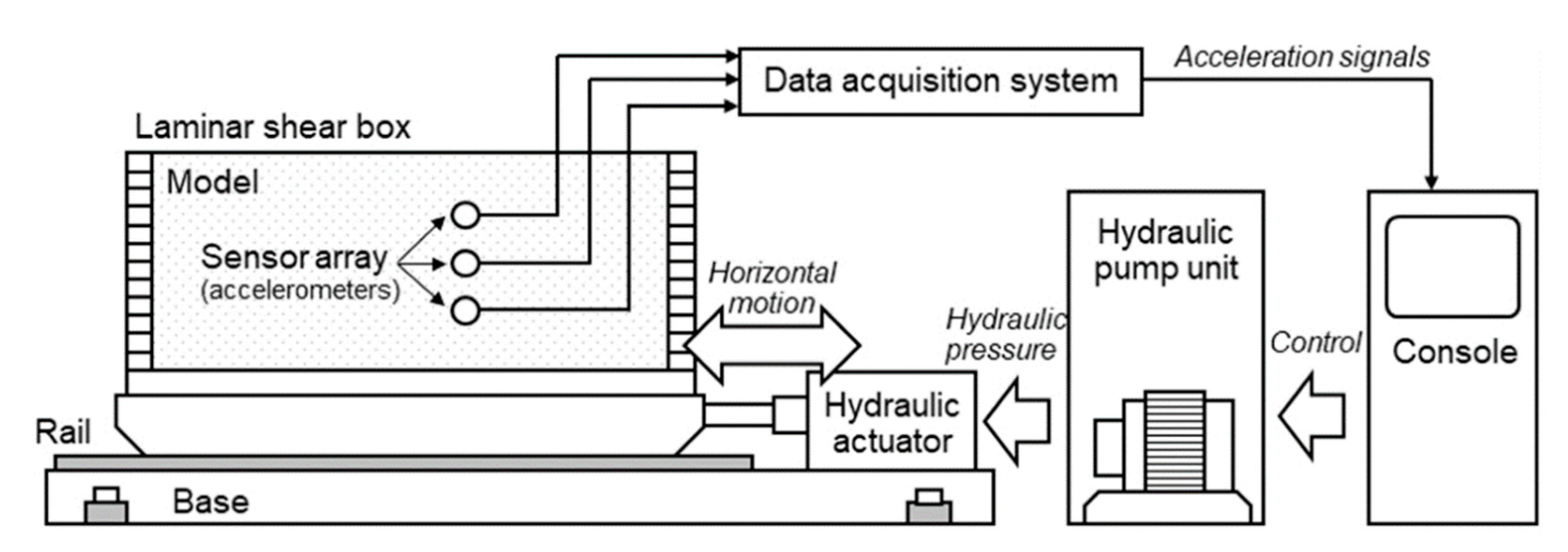
2.2.1. 1 g Shaking Table Test Equipment System
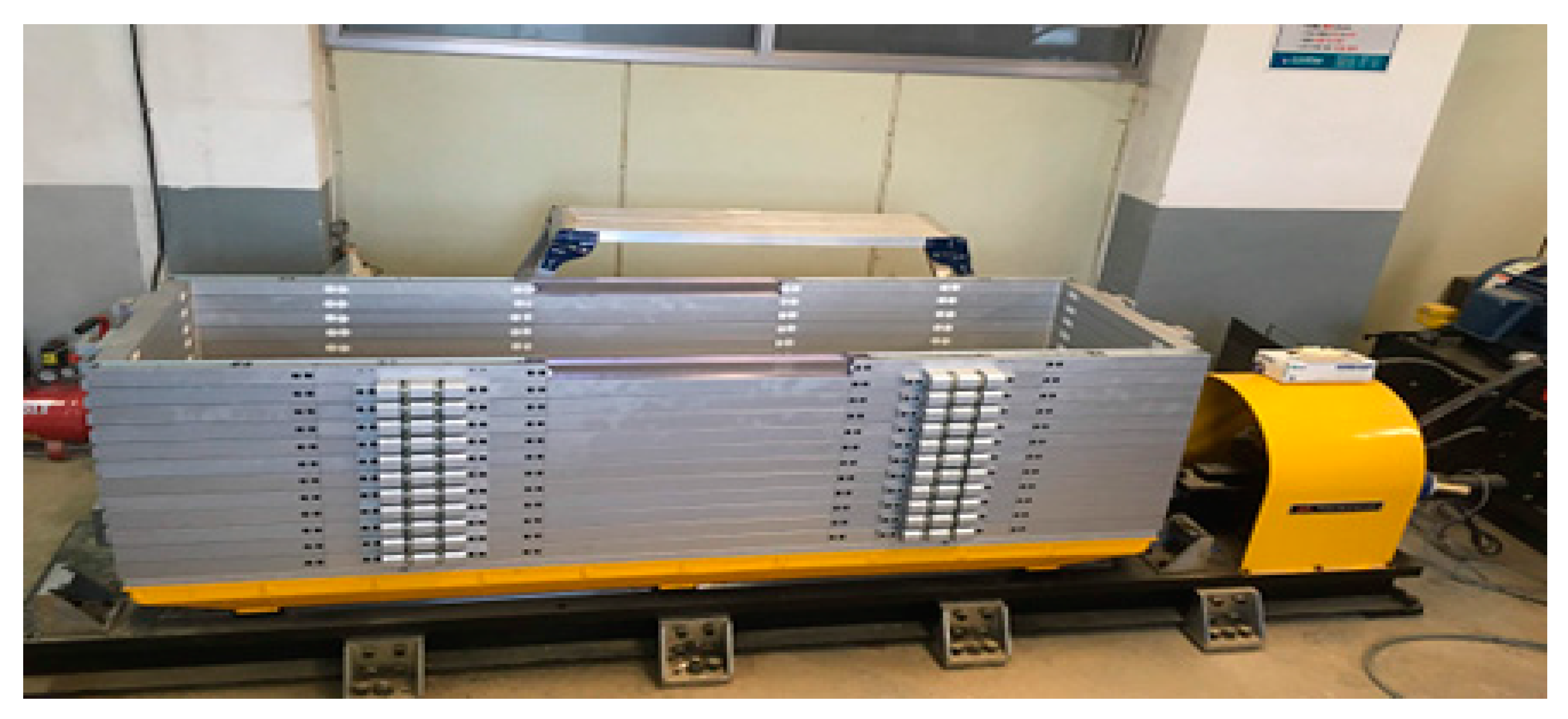
2.2.2. Laminar Shear Box
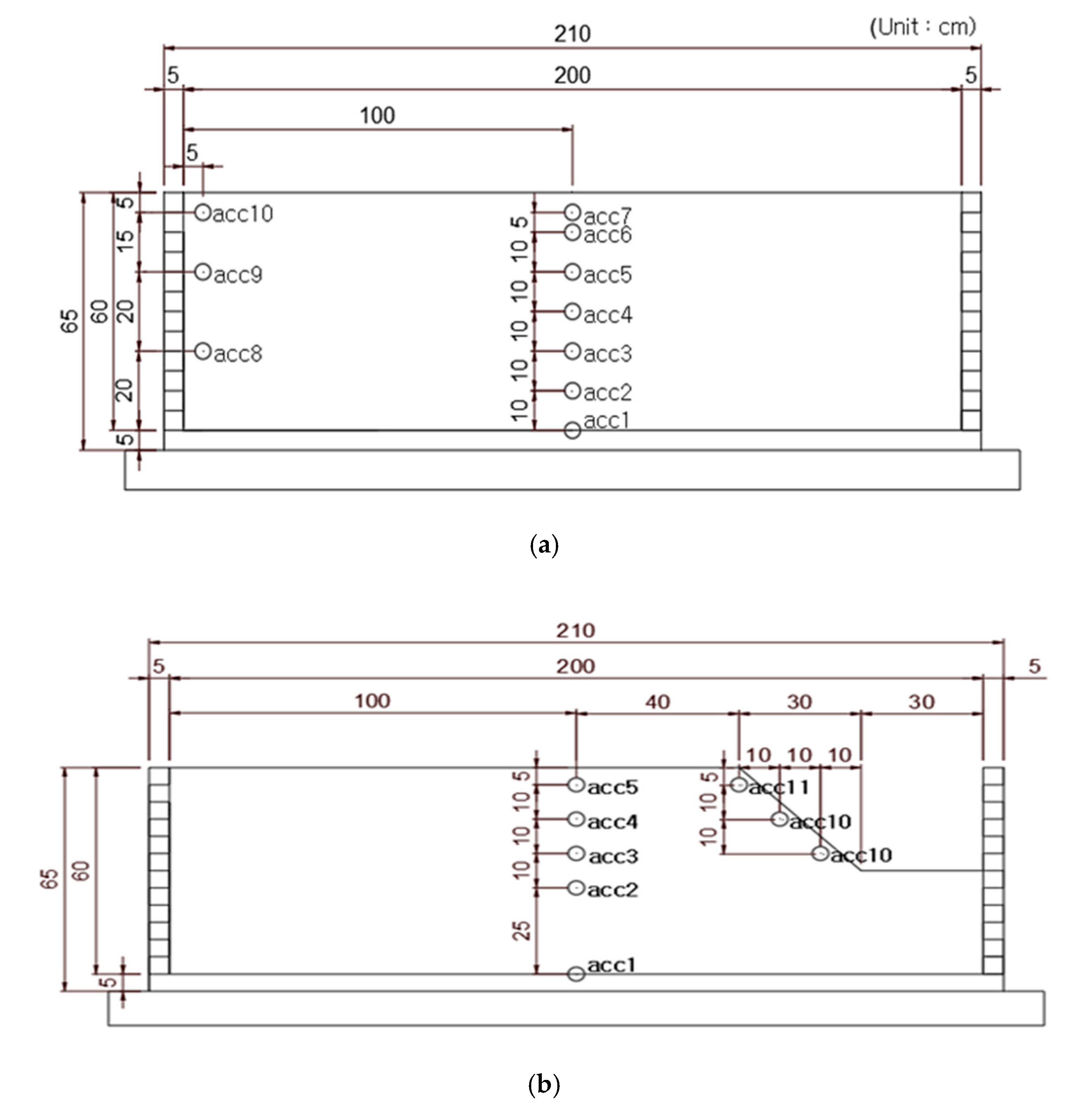
2.2.3. Accelerometer
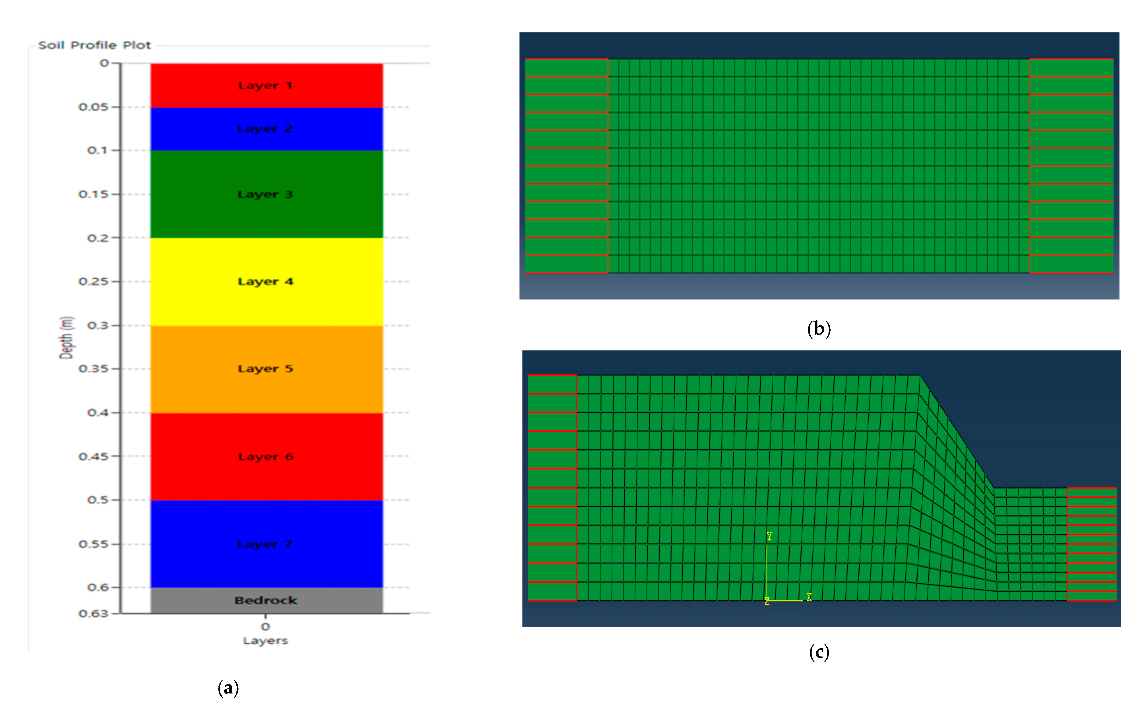
2.3. Numerical Simulation Method
2.3.1. DEEPSOIL Software
2.3.2. ABAQUS Software
2.3.3. Comparison of DEEPSOIL and ABAQUS Software
Boundary Conditions
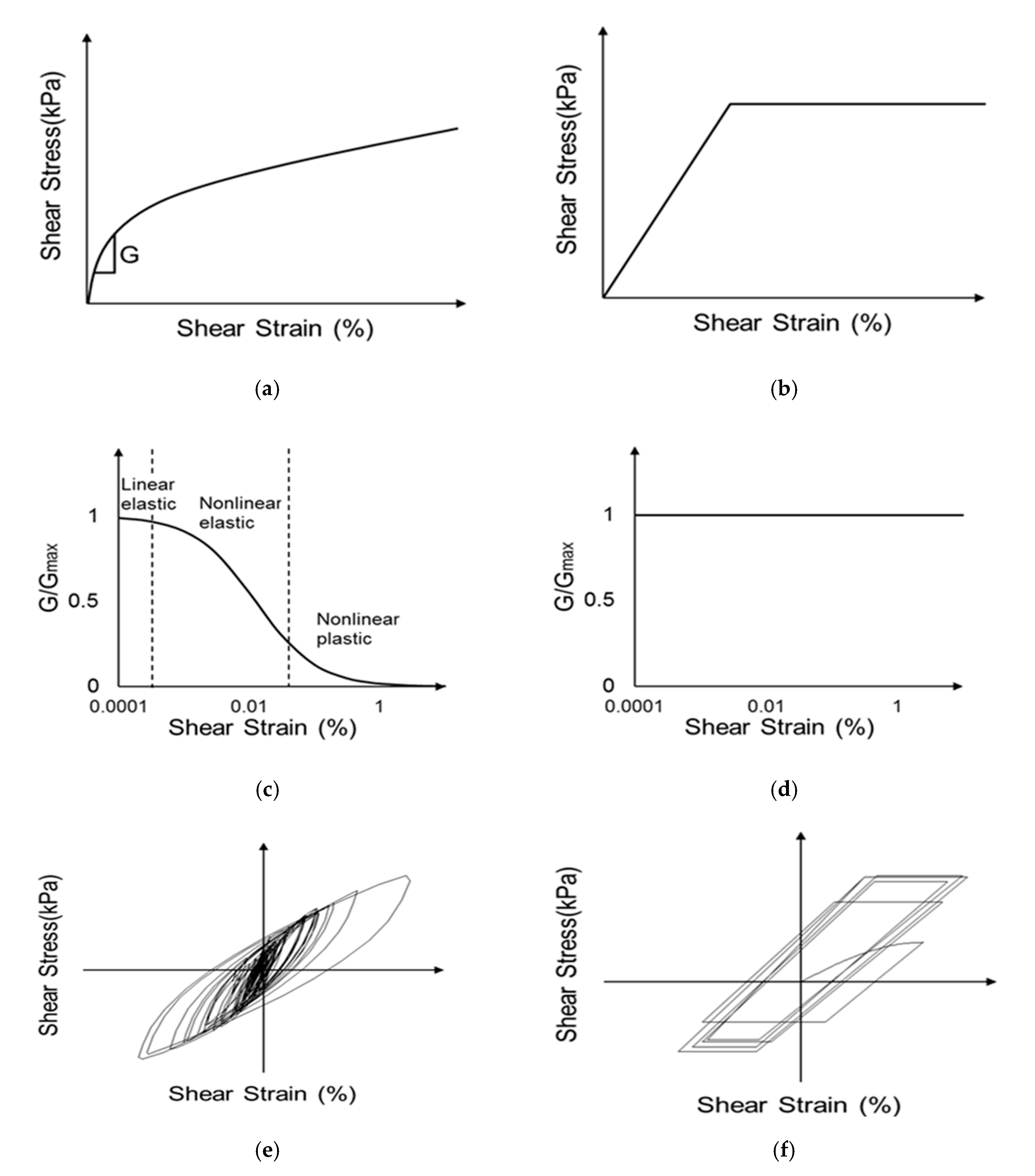
Constitutive Models
3. Comparison and Analysis of Acceleration Response Results
3.1. Comparison of Flat Ground with Normal Elastic Modulus
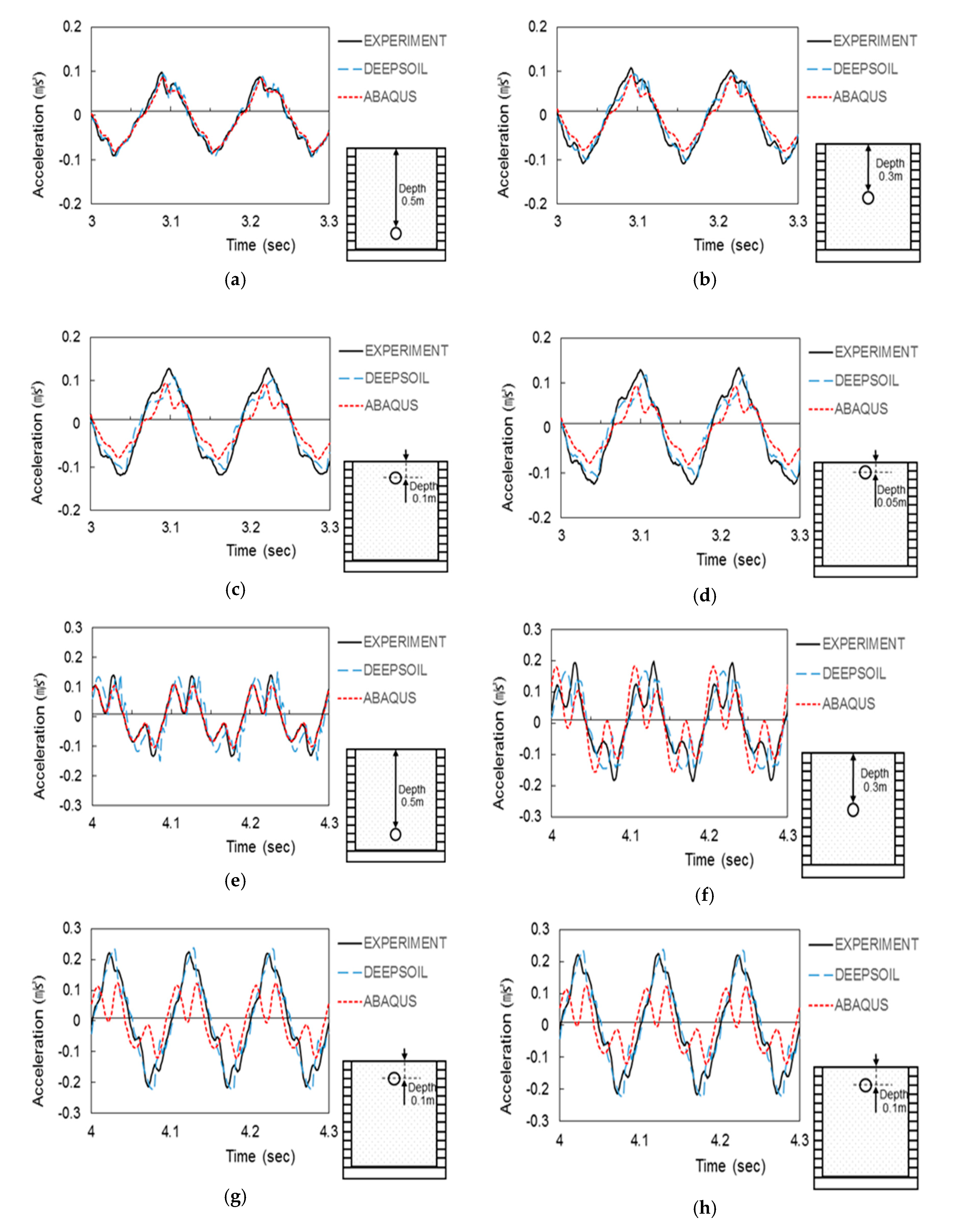
3.1.1. Acceleration-Time History
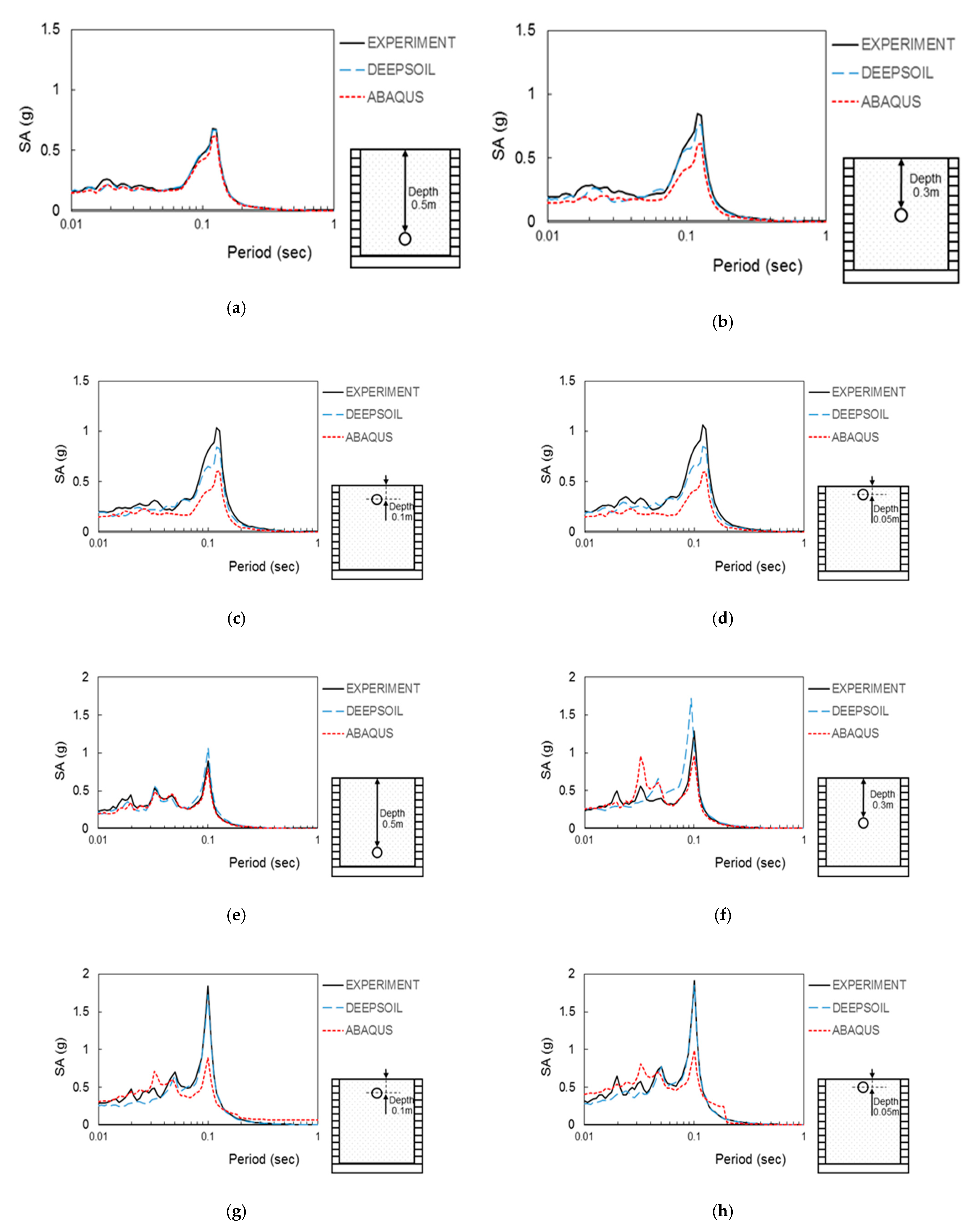
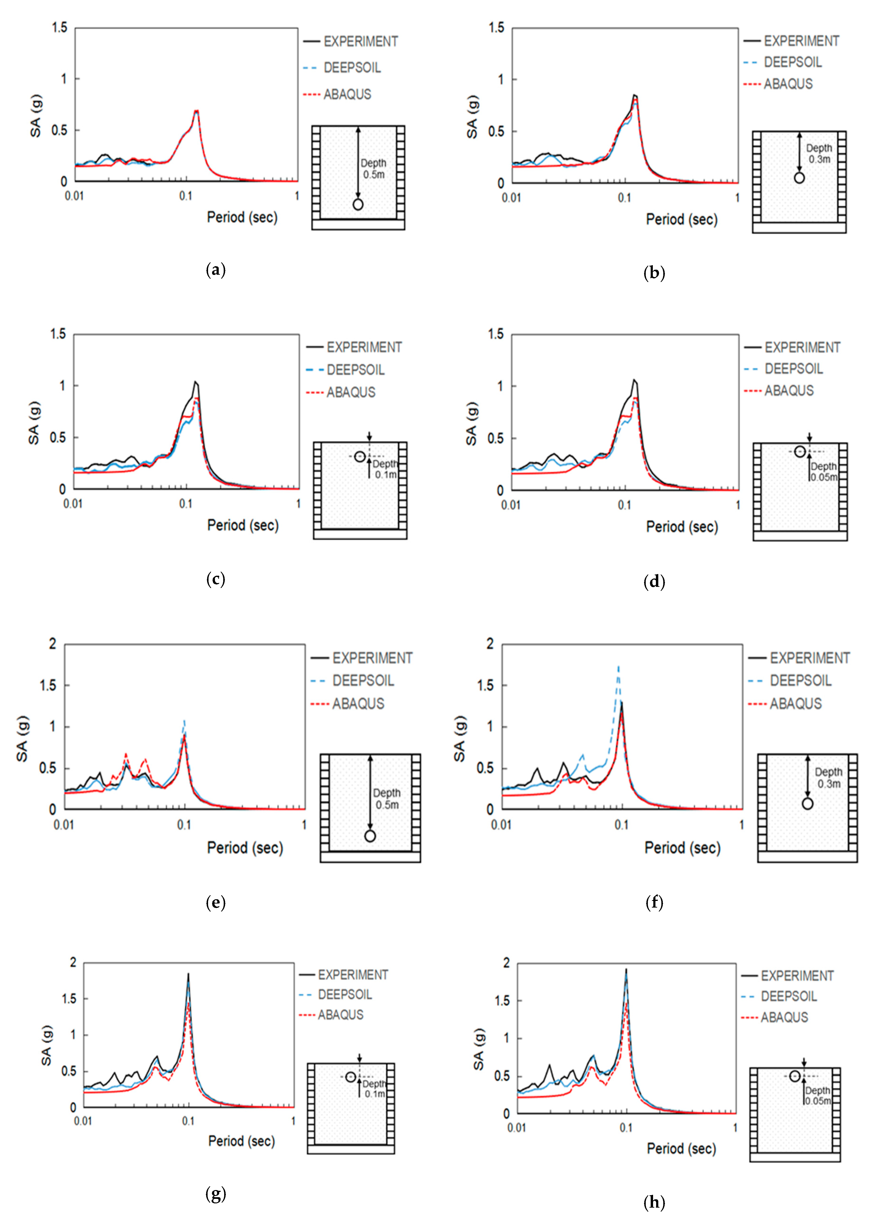
3.1.2. Spectral Acceleration
3.2. Comparison of Flat Ground with Adjusted Elastic Modulus
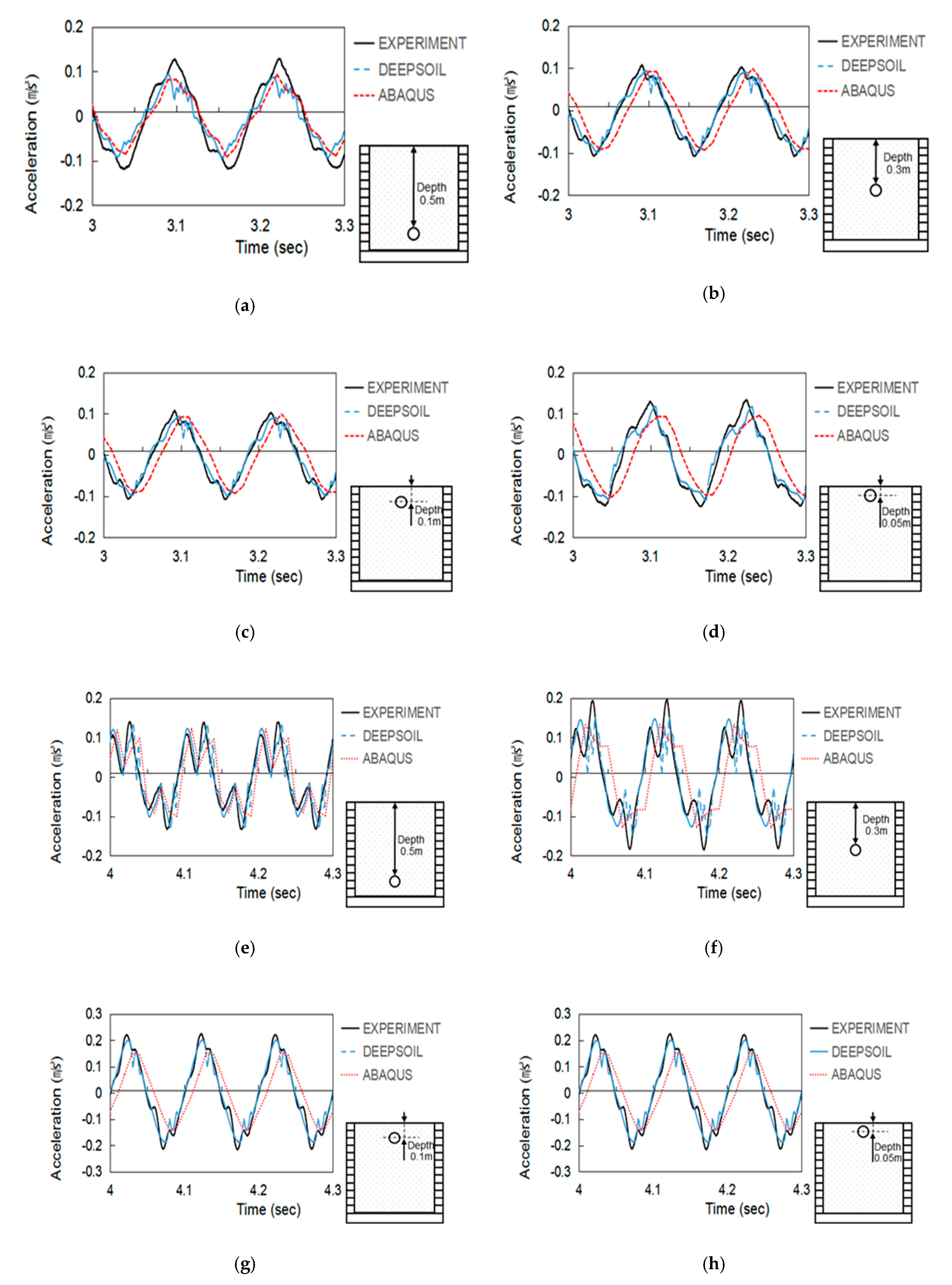
3.2.1. Acceleration-Time History
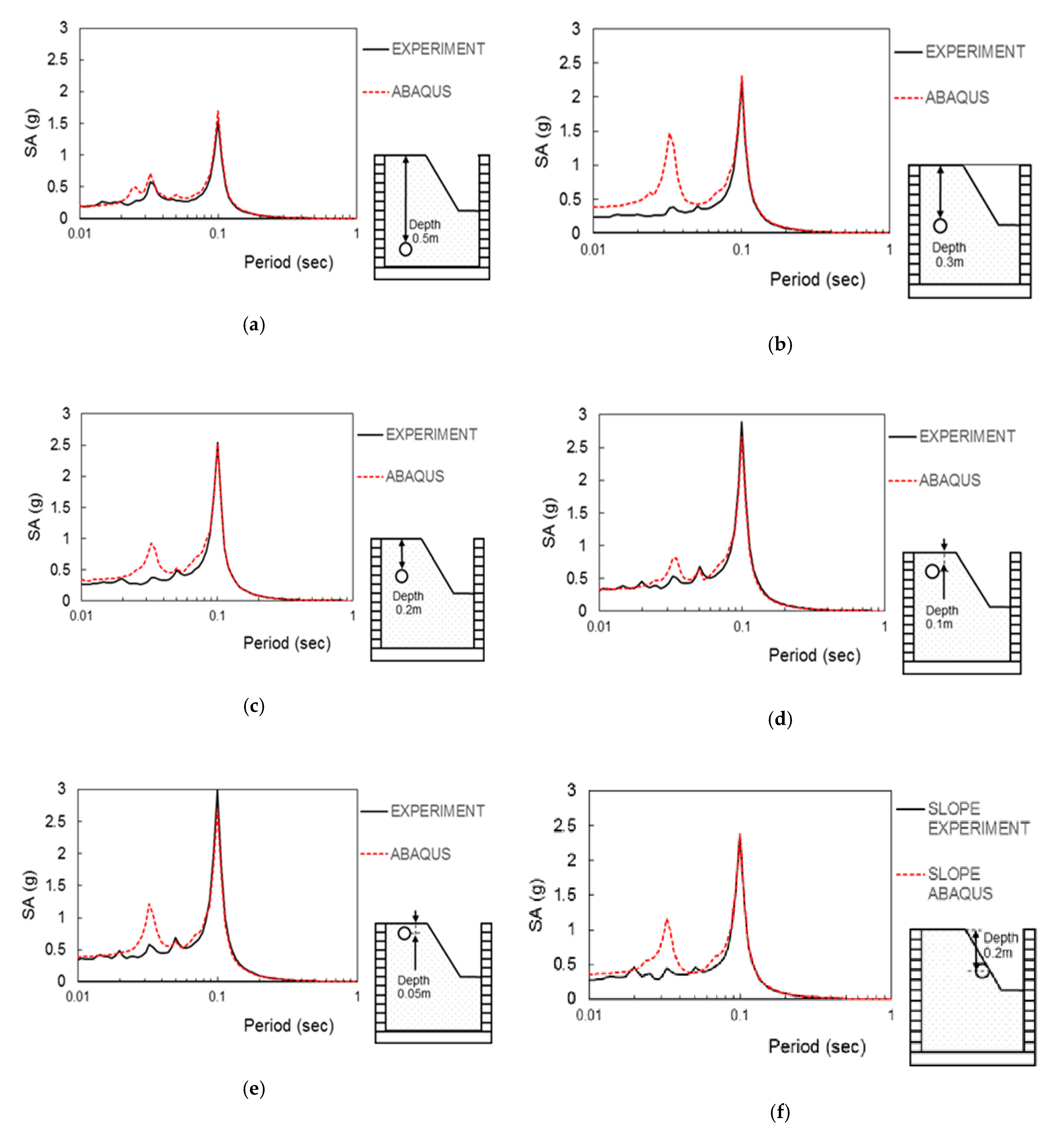
3.2.2. Spectral Acceleration
3.3. Comparison of Slope with Adjusted Elastic Modulus
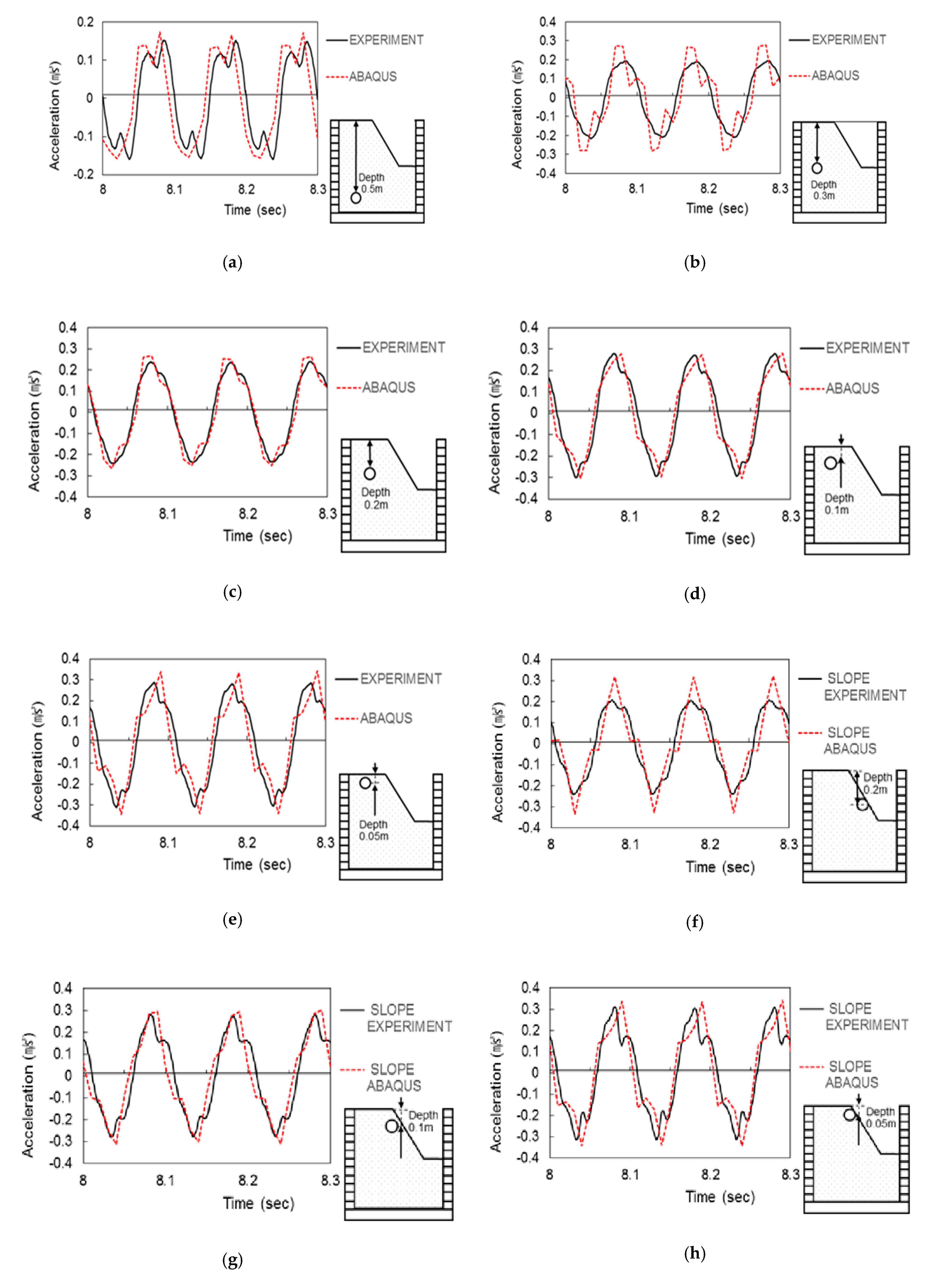
3.3.1. Acceleration-Time History
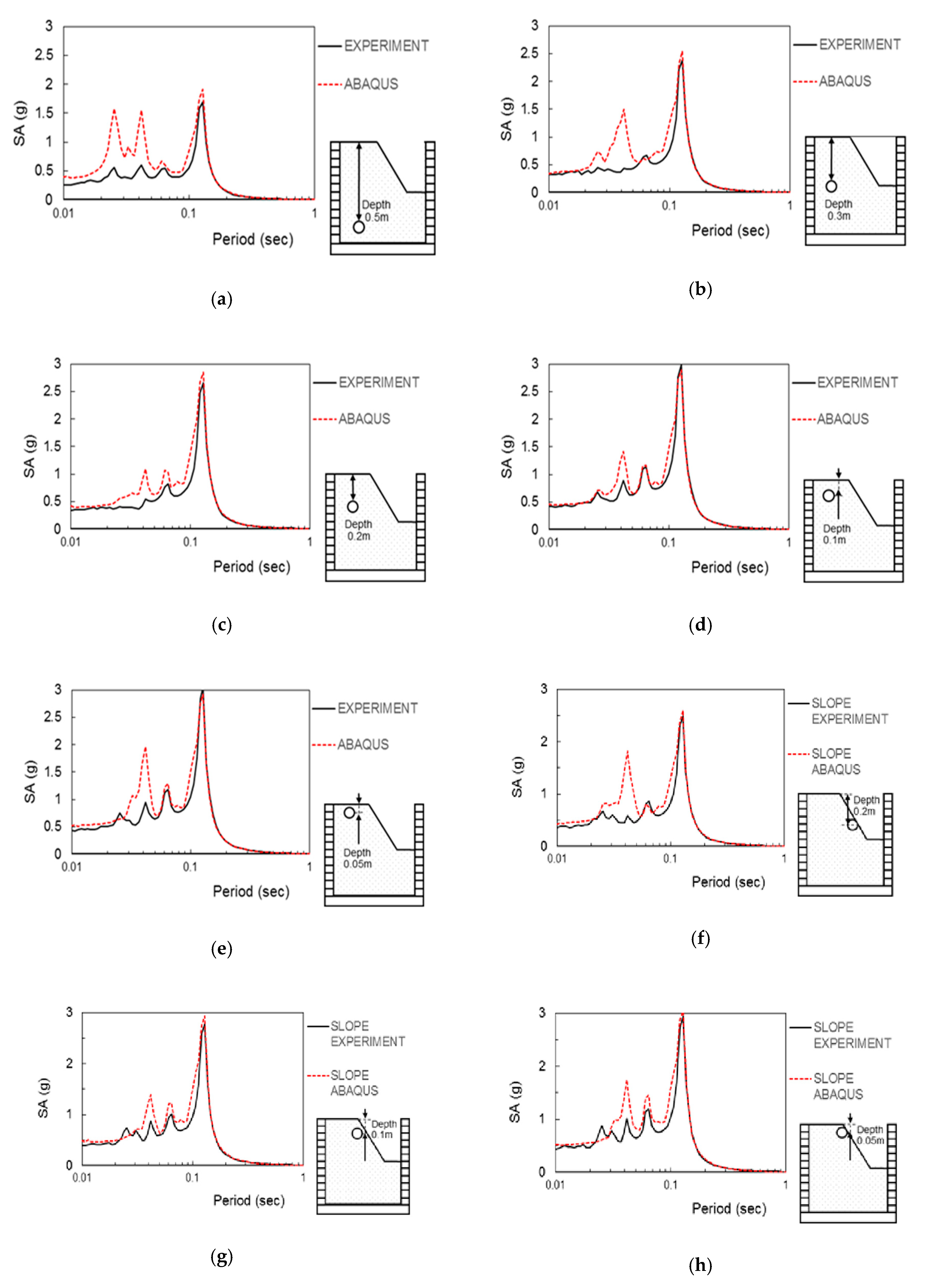
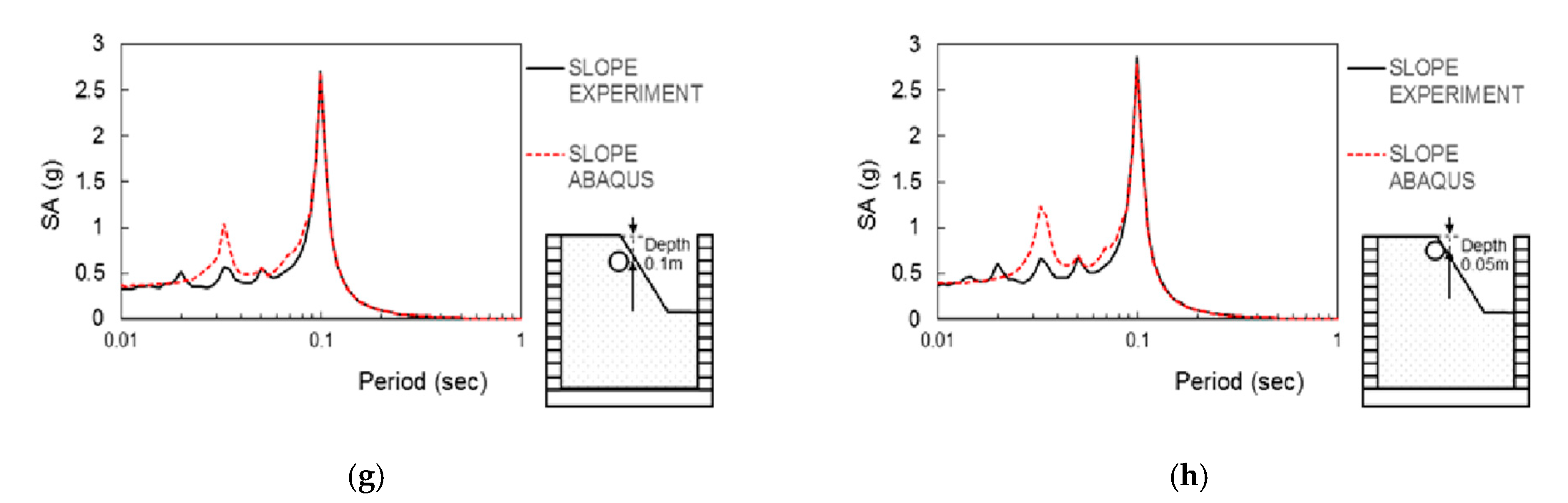
3.3.2. Spectral Acceleration
4. Summary and Conclusions
Author Contributions
Funding
Institutional Review Board Statement
Informed Consent Statement
Data Availability Statement
Conflicts of Interest
References
- Jafarzadeh, B. Design and Evaluation Concepts of Laminar Shear Box for 1 g Shaking Table Tests. In Proceedings of the 13th World Conference on Earthquake Engineering, Vancouver, BC, Canada, 1–6 August 2004. Paper No. 1391. [Google Scholar]
- Chen, G.X.; Wang, Z.H.; Zuo, X.; Du, X.L.; Han, X.J. Development of laminar shear soil container for shaking table tests. Chin. J. Geotech. Eng. 2010, 32, 89–97. [Google Scholar]
- Turan, A.; Hinchberger, S.D.; El Naggar, H. Design and commissioning of a laminar soil container for use on small shaking tables. Soil Dyn. Earthq. Eng. 2009, 29, 404–414. [Google Scholar] [CrossRef]
- Lee, C.J.; Wei, Y.C.; Kuo, Y.C. Boundary effects of a laminar container in centrifuge shaking table tests. Soil Dyn. Earthq. Eng. 2012, 34, 37–51. [Google Scholar] [CrossRef]
- Andersen, S.; Andersen, L. Modelling of landslides with the material-point method. Comput. Geosci. 2010, 14, 137–147. [Google Scholar] [CrossRef]
- Faris, F.; Fawu, W. Investigation of the initiation mechanism of an earthquake-induced landslide during rainfall: A case study of the Tandikat landslide, West Sumatra, Indonesia. Geoenviron. Disasters 2014, 1, 4. [Google Scholar] [CrossRef]
- Cheng, X.; Cui, C.; Sun, Z.; Xia, J.; Wang, G. Shaking Table Test and Numerical Verification for Free Ground Seismic Response of Saturated Soft Soil. Math. Probl. Eng. 2018, 2018. [Google Scholar] [CrossRef]
- Moghadam, M.R.; Baziar, M.H. Seismic ground motion amplification pattern induced by a subway tunnel: Shaking table testing and numerical simulation. Soil Dyn. Earthq. Eng. 2016, 83, 81–97. [Google Scholar] [CrossRef]
- Meyerhof, G.G. Penetration tests and bearing capacity of cohesionless soils. J. Soil Mech. Found. Div. 1956, 82, 1–19. [Google Scholar] [CrossRef]
- Hardin, B.O.; Richart, F.E. Elastic wave velocities in granular soils. J. Soil Mech. Found. Div. 1963, 89, 33–65. [Google Scholar] [CrossRef]
- Kim, H.; Jin, Y.; Lee, Y.; Kim, H.; Kim, D. Dynamic Response Characteristics of Embankment Model for Various Slope Angles. J. Korean Geosynth. Soc. 2020, 19, 35–46. [Google Scholar] [CrossRef]
- Darendeli, M.B. Development of a New Family of Normalized Modulus Reduction and Material Damping Curves. Ph.D. Thesis, University of Texas, Austin, TX, USA, 2001. [Google Scholar]
- Geotechdata Info. Soil Young’s Modulus. Available online: http://geotechdata.info/parameter/soil-young-s-modulus (accessed on 23 October 2020).


| Parameter | Value | Parameter | Value |
|---|---|---|---|
| No.200 Passing (%) | 10.8 | emax | 1.123 |
| Gs | 2.69 | emin | 0.443 |
| OMC (%) | 12.5 | rd max (kN/m3) | 18.27 |
| PI (%) | NP | rd min (kN/m3) | 12.43 |
| USCS | SW-SM | Elastic modulus (Pa) | 2 × 10⁸ |
| Internal friction angle (°) | 27.7° | Dilatancy angle (°) | 24.4° |
| USCS | Description | Loose (MPa) | Medium (MPa) | Dense (MPa) |
|---|---|---|---|---|
| GW, SW | Gravels/Sand well-graded | 30–80 | 80–160 | 160–320 |
| SP | Sand, uniform | 10–30 | 30–50 | 50–80 |
| GM, SM | Sand/Gravel silly | 7–12 | 12–20 | 20–30 |
Publisher’s Note: MDPI stays neutral with regard to jurisdictional claims in published maps and institutional affiliations. |
© 2021 by the authors. Licensee MDPI, Basel, Switzerland. This article is an open access article distributed under the terms and conditions of the Creative Commons Attribution (CC BY) license (http://creativecommons.org/licenses/by/4.0/).
Share and Cite
Jin, Y.; Kim, H.; Kim, D.; Lee, Y.; Kim, H. Seismic Response of Flat Ground and Slope Models through 1 g Shaking Table Tests and Numerical Analysis. Appl. Sci. 2021, 11, 1875. https://doi.org/10.3390/app11041875
Jin Y, Kim H, Kim D, Lee Y, Kim H. Seismic Response of Flat Ground and Slope Models through 1 g Shaking Table Tests and Numerical Analysis. Applied Sciences. 2021; 11(4):1875. https://doi.org/10.3390/app11041875
Chicago/Turabian StyleJin, Yong, Hoyeon Kim, Daehyeon Kim, Yonghee Lee, and Haksung Kim. 2021. "Seismic Response of Flat Ground and Slope Models through 1 g Shaking Table Tests and Numerical Analysis" Applied Sciences 11, no. 4: 1875. https://doi.org/10.3390/app11041875
APA StyleJin, Y., Kim, H., Kim, D., Lee, Y., & Kim, H. (2021). Seismic Response of Flat Ground and Slope Models through 1 g Shaking Table Tests and Numerical Analysis. Applied Sciences, 11(4), 1875. https://doi.org/10.3390/app11041875